
Modelling the Event-Based Hydrological Response of Mediterranean Forests to Prescribed Fire and Soil Mulching with Fern Using the Curve Number, Horton and USLE-Family (Universal Soil Loss Equation) Models

 , , , and
Abstract
:1. Introduction
2. Materials and Methods
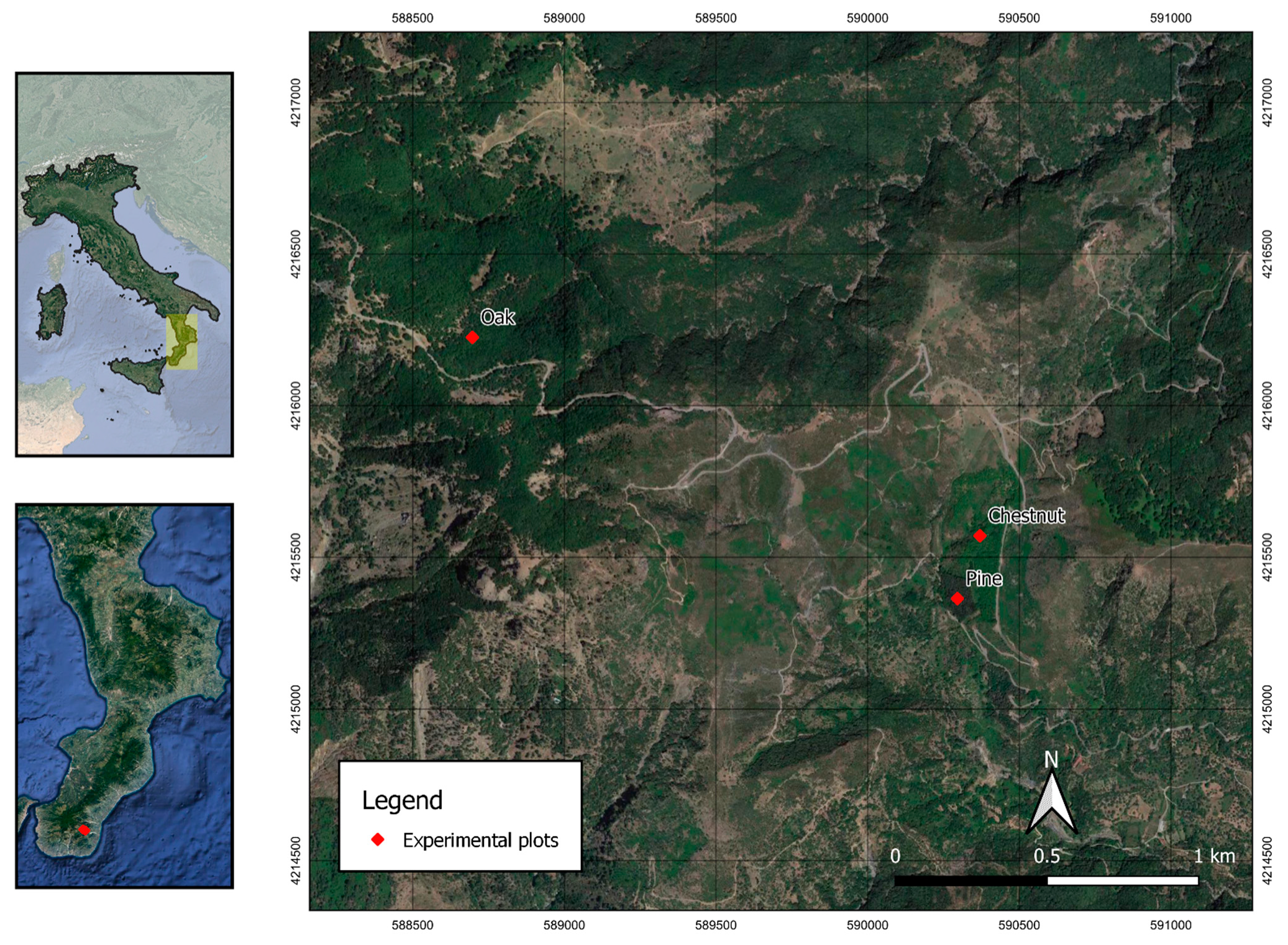
2.1. Study Area
- a pine (Pinus pinaster Aiton, “Calamacia” site, 38°4′52″ N; 16°1′46″ E) stand reforested in 1984 over an area between 650 and 700 m a.s.l.
- a natural oak (Quercus frainetto Ten., “Rungia” site, 38°5′20″ N; 16°0′39″ E) stand (900–950 m a.s.l.)
- a chestnut stand (Castanea sativa Mill., “Orgaro” site, 38°4′59″ N; 16°1′50″ E) about 30 years-old, between 700 and 750 m.
2.2. Prescribed Fire Operations and Mulching Application
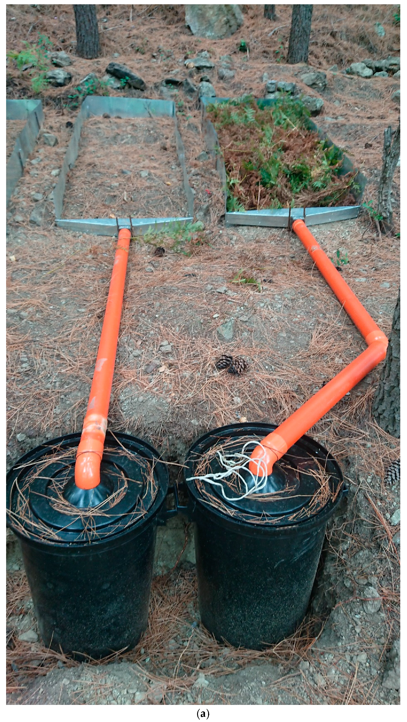
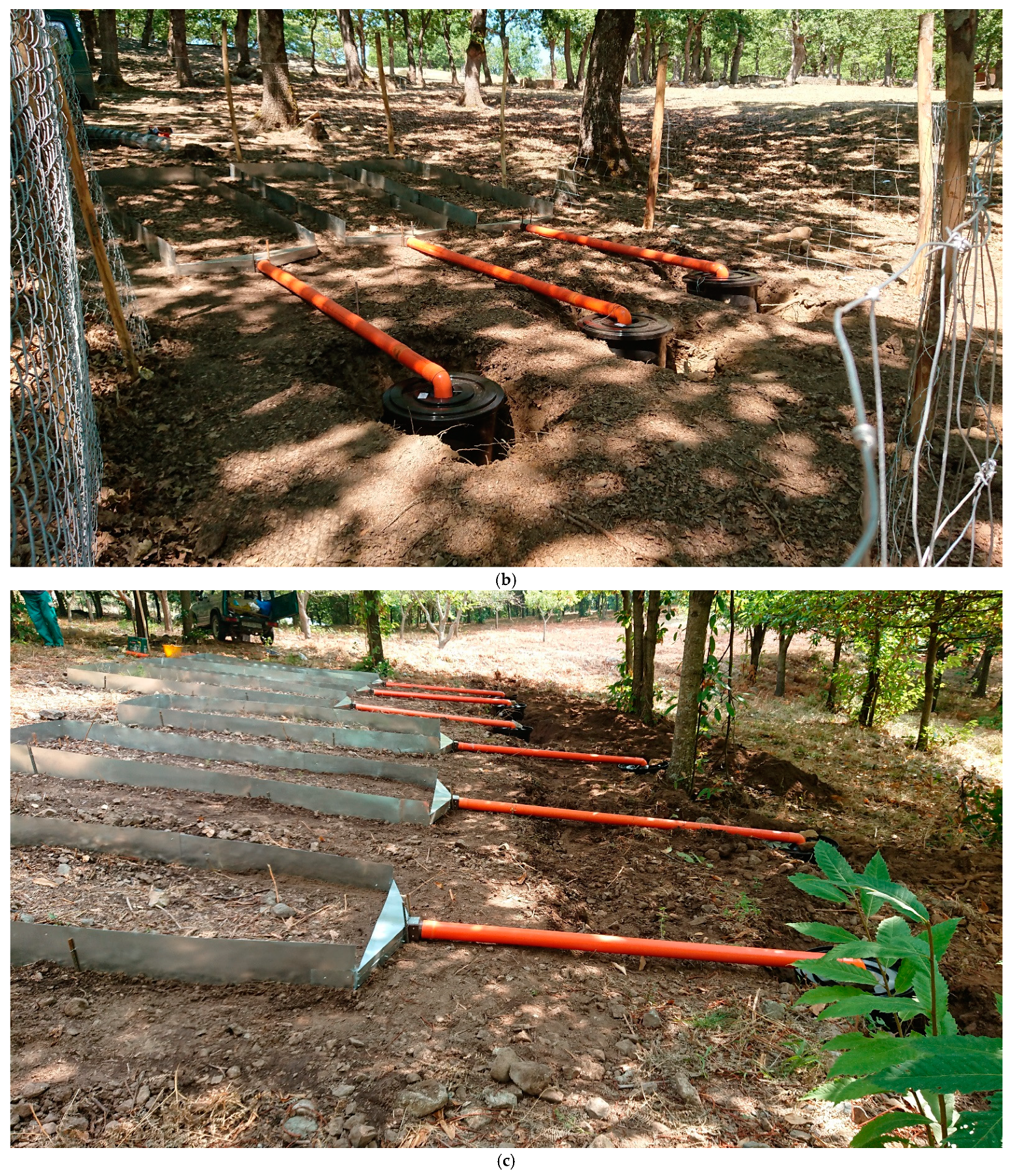
2.3. Hydrological Monitoring
2.4. Short Description of the Models
2.4.1. SCS-CN Model
- AMCI: dry condition and minimum surface runoff
- AMCII: average condition and surface runoff
- AMCIII: wet condition and maximum surface runoff.
2.4.2. Horton Equation
2.4.3. MUSLE Equation
2.4.4. USLE-M Equation
2.5. Model Implementation in the Experimental Plots
2.5.1. SCS-CN Model
2.5.2. Horton Equation
2.5.3. MUSLE Equation
2.5.4. USLE-M Equation
2.6. Model Calibration
2.7. Model Performance Evaluation
3. Results and Discussions
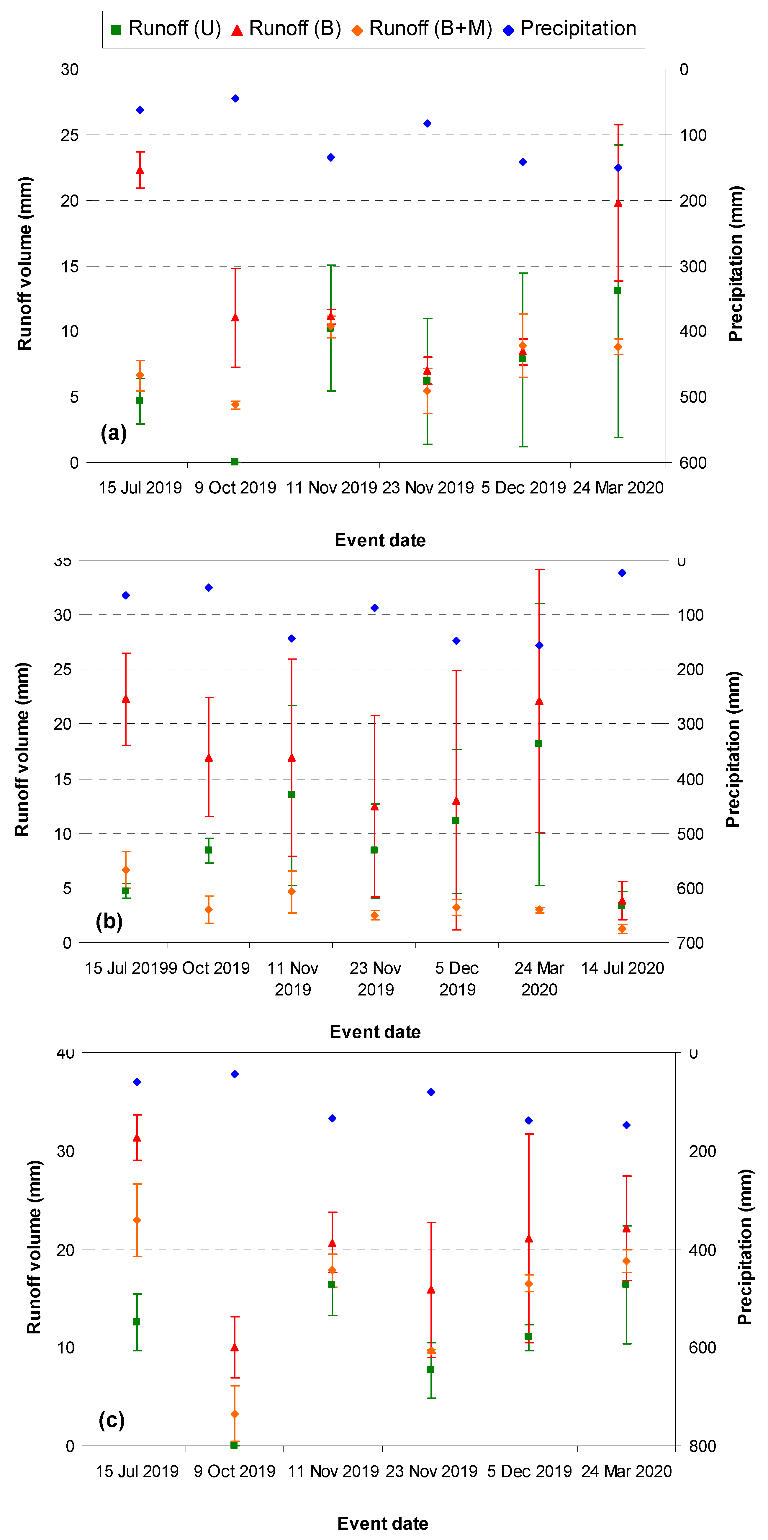
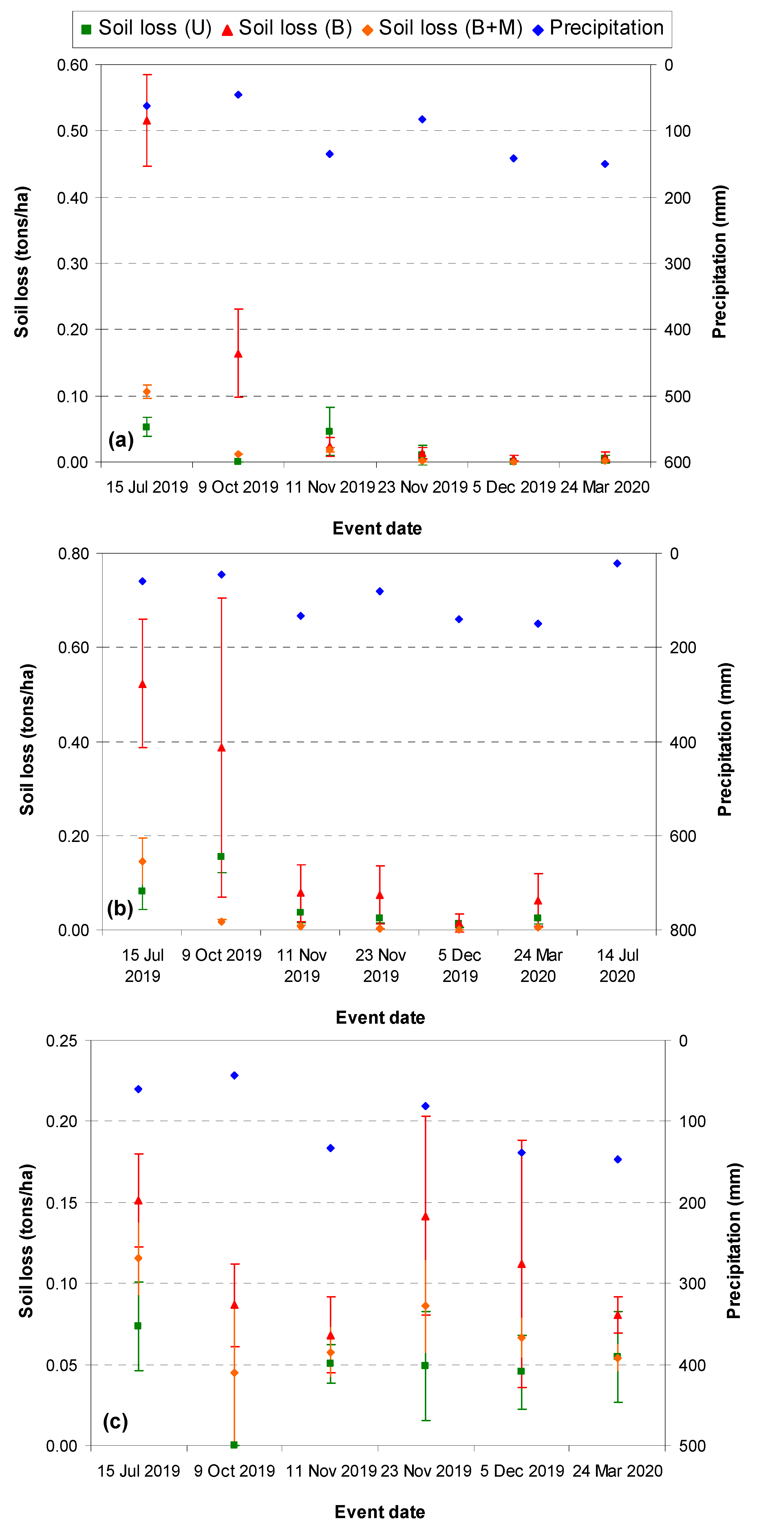
3.1. Hydrological Characterization
3.2. Hydrological Modeling
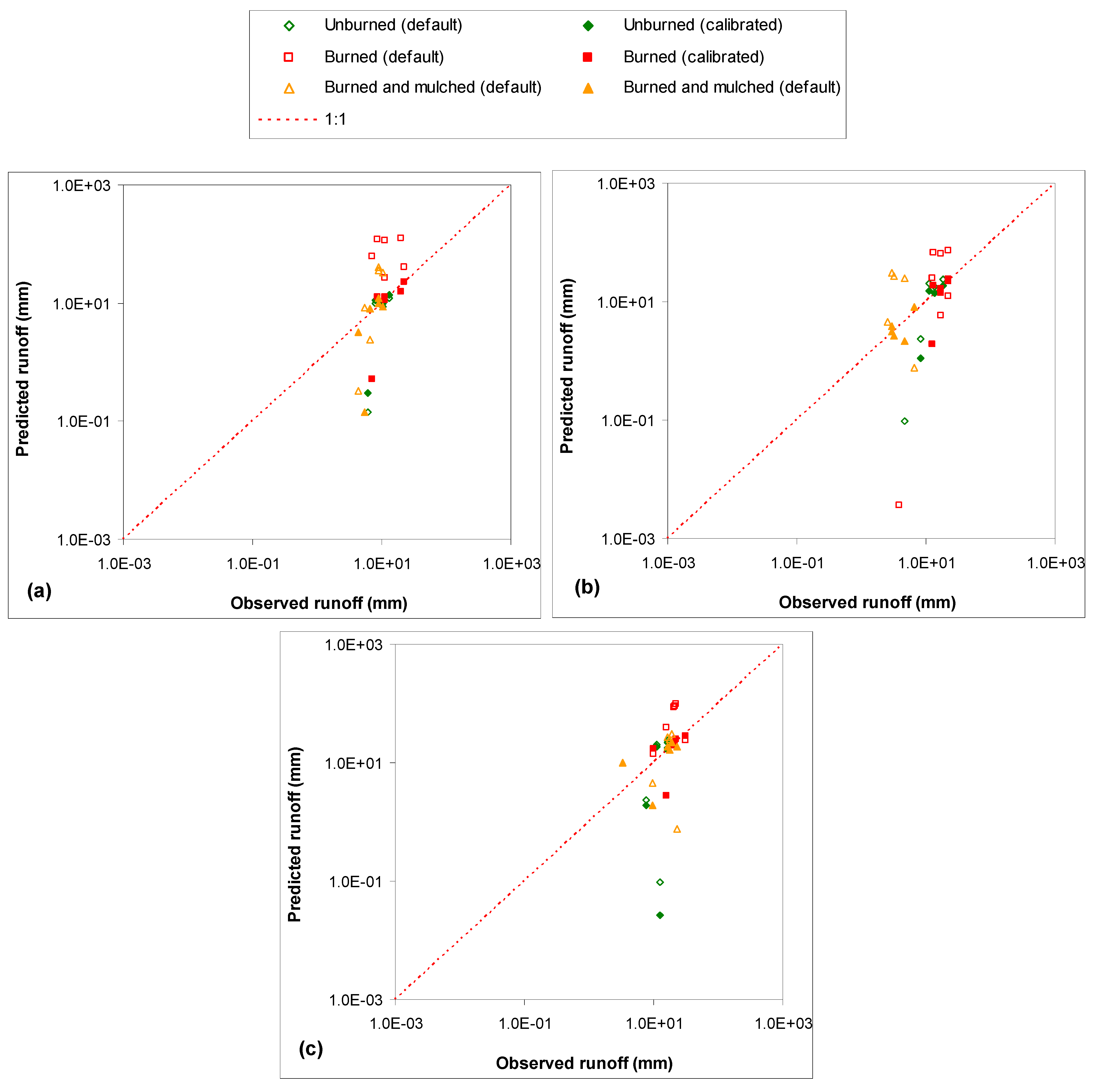
3.2.1. SCS-CN Model
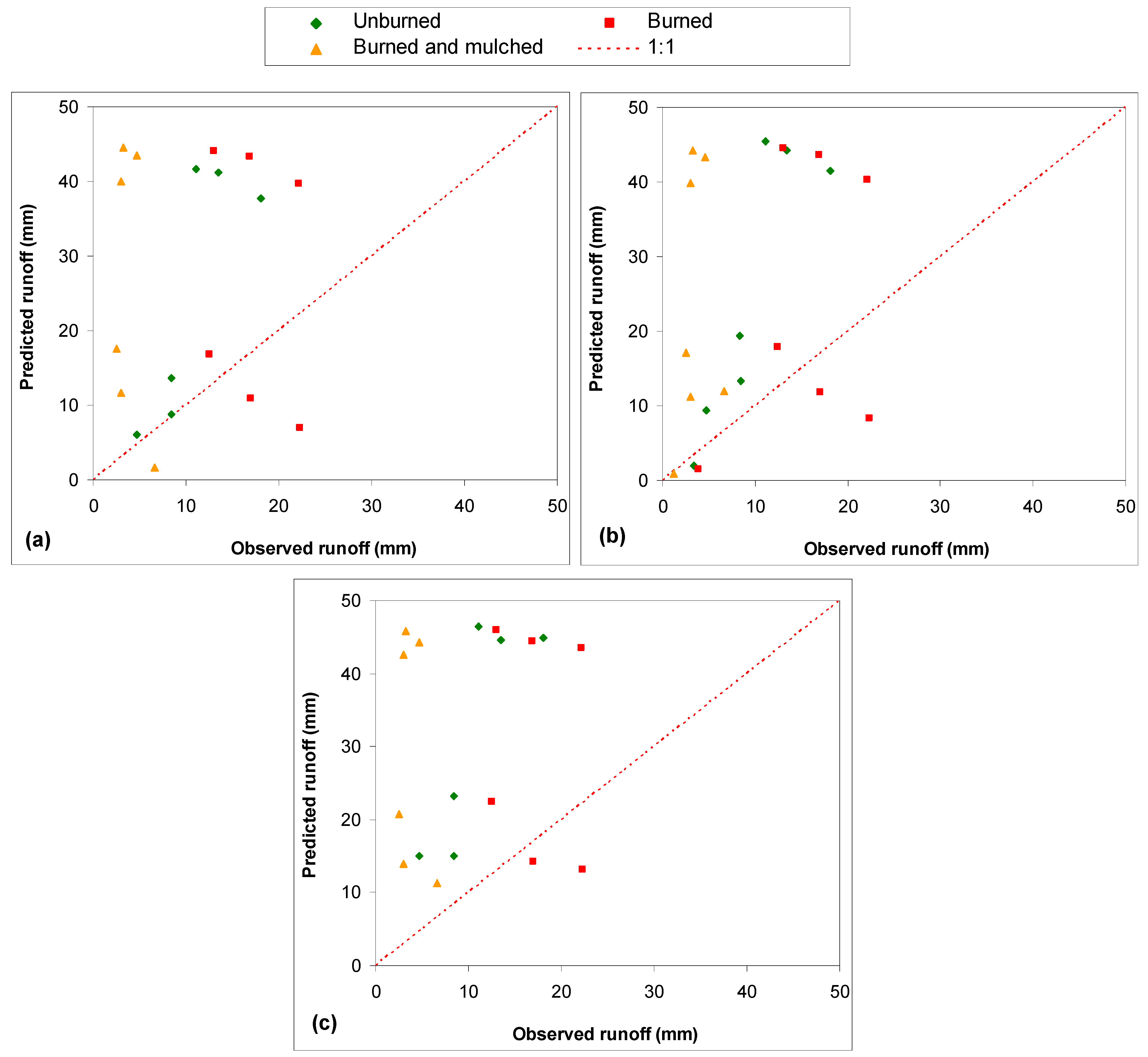
3.2.2. Horton Model
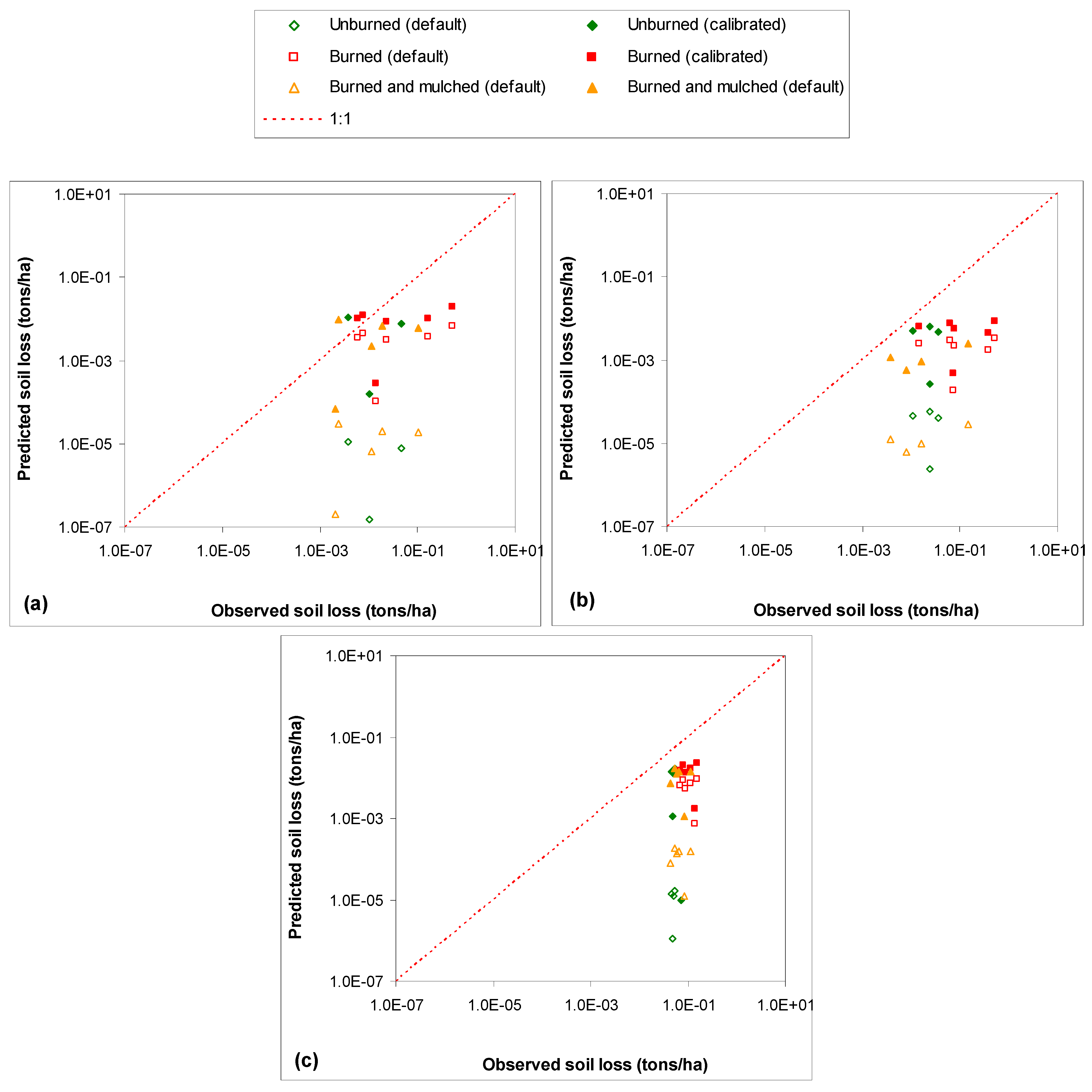
3.2.3. MUSLE Model
3.2.4. USLE-M Model
4. Conclusions
- for runoff modelling CNs of 80, 83, and 79 (burned soils) and 65, 76, and 65 (burned and mulched soils) throughout the two to three months after fire, and 45, 47, and 41 (burned soils) and 32, 45, and 39 (burned and mulched soils) in the following period, for chestnut, oak, and pine forests, respectively;
- for soil loss predictions C-factors of 0.521, 0.085, and 0.339 (burned soils) and 0.069, 0.060, and 0.040 (burned and mulched soils) immediately after a fire, and 0.052, 0.059, and 0.008 (burned soils) and 0.007, 0.050, and 0.001 (burned and mulched soils) in the following period, for chestnut, oak, and pine forests, respectively.
Author Contributions
Funding
Institutional Review Board Statement
Data Availability Statement
Acknowledgments
Conflicts of Interest
References
- Kozlowski, T.T. Fire and ecosystems. Elsevier: Amsterdam, The Netherlands, 2012. [Google Scholar]
- Moody, J.A.; Shakesby, R.A.; Robichaud, P.R.; Cannon, S.H.; Martin, D.A. Current Research Issues Related to Post-Wildfire Runoff and Erosion Processes. Earth-Sci. Rev. 2013, 122, 10–37. [Google Scholar] [CrossRef]
- Zavala, L.M.; De Celis, R.; Jordán, A. How Wildfires Affect Soil Properties. A Brief Review. Cuad. Investig. Geográfica 2014, 40, 311. [Google Scholar] [CrossRef] [Green Version]
- Zema, D.A. Postfire Management Impacts on Soil Hydrology. Curr. Opin. Environ. Sci. Health 2021, 21, 100252. [Google Scholar] [CrossRef]
- Pausas, J.G.; Fernández-Muñoz, S. Fire Regime Changes in the Western Mediterranean Basin: From Fuel-Limited to Drought-Driven Fire Regime. Clim. Chang. 2012, 110, 215–226. [Google Scholar] [CrossRef] [Green Version]
- Morán-Ordóñez, A.; Duane, A.; Gil-Tena, A.; De Cáceres, M.; Aquilué, N.; Guerra, C.A.; Geijzendorffer, I.R.; Fortin, M.; Brotons, L. Future Impact of Climate Extremes in the Mediterranean: Soil Erosion Projections When Fire and Extreme Rainfall Meet. Land Degrad. Dev. 2020, 31, 3040–3054. [Google Scholar] [CrossRef]
- Diodato, N.; Bellocchi, G. MedREM, a Rainfall Erosivity Model for the Mediterranean Region. J. Hydrol. 2010, 387, 119–127. [Google Scholar] [CrossRef]
- Giorgi, F.; Lionello, P. Climate Change Projections for the Mediterranean Region. Glob. Planet. Chang. 2008, 63, 90–104. [Google Scholar] [CrossRef]
- Lucas-Borja, M.E. Efficiency of Postfire Hillslope Management Strategies: Gaps of Knowledge. Curr. Opin. Environ. Sci. Health 2021, 21, 100247. [Google Scholar] [CrossRef]
- Neary, D.G.; Leonard, J.M. Restoring fire to forests: Contrasting the effects on soils of prescribed fire and wildfire. In Soils and Landscape Restoration; Elsevier: Amsterdam, The Netherlands, 2021; pp. 333–355. [Google Scholar]
- Vega, J.A.; Fernández, C.; Fonturbel, T. Throughfall, Runoff and Soil Erosion after Prescribed Burning in Gorse Shrubland in Galicia (NW Spain). Land Degrad. Dev. 2005, 16, 37–51. [Google Scholar] [CrossRef]
- Alcañiz, M.; Outeiro, L.; Francos, M.; Úbeda, X. Effects of Prescribed Fires on Soil Properties: A Review. Sci. Total Environ. 2018, 613, 944–957. [Google Scholar] [CrossRef]
- Rulli, M.C.; Offeddu, L.; Santini, M. Modeling Post-Fire Water Erosion Mitigation Strategies. Hydrol. Earth Syst. Sci. 2013, 17, 2323–2337. [Google Scholar] [CrossRef] [Green Version]
- Prosdocimi, M.; Tarolli, P.; Cerdà, A. Mulching practices for reducing soil water erosion: A review. Earth-Sci. Rev. 2016, 161, 191–203. [Google Scholar]
- Nunes, J.P.; Naranjo Quintanilla, P.; Santos, J.M.; Serpa, D.; Carvalho-Santos, C.; Rocha, J.; Keizer, J.J.; Keesstra, S.D. Afforestation, Subsequent Forest Fires and Provision of Hydrological Services: A Model-Based Analysis for a Mediterranean Mountainous Catchment: Mediterranean Afforestation, Forest Fires and Hydrological Services. Land Degrad. Develop. 2018, 29, 776–788. [Google Scholar] [CrossRef]
- Filianoti, P.; Gurnari, L.; Zema, D.A.; Bombino, G.; Sinagra, M.; Tucciarelli, T. An Evaluation Matrix to Compare Computer Hydrological Models for Flood Predictions. Hydrology 2020, 7, 42. [Google Scholar] [CrossRef]
- Fernández, C.; Vega, J.A. Evaluation of RUSLE and PESERA Models for Predicting Soil Erosion Losses in the First Year after Wildfire in NW Spain. Geoderma 2016, 273, 64–72. [Google Scholar] [CrossRef]
- Bezak, N.; Mikoš, M.; Borrelli, P.; Alewell, C.; Alvarez, P.; Anache, J.A.A.; Baartman, J.; Ballabio, C.; Biddoccu, M.; Cerdà, A. Soil Erosion Modelling: A Bibliometric Analysis. Environ. Res. 2021, 197, 111087. [Google Scholar] [CrossRef]
- Borrelli, P.; Alewell, C.; Alvarez, P.; Anache, J.A.A.; Baartman, J.; Ballabio, C.; Bezak, N.; Biddoccu, M.; Cerdà, A.; Chalise, D. Soil Erosion Modelling: A Global Review and Statistical Analysis. Sci. Total Environ. 2021, 780, 146494. [Google Scholar] [CrossRef] [PubMed]
- Aksoy, H.; Kavvas, M.L. A Review of Hillslope and Watershed Scale Erosion and Sediment Transport Models. Catena 2005, 64, 247–271. [Google Scholar] [CrossRef]
- Lucas-Borja, M.E.; Bombino, G.; Carrà, B.G.; D’Agostino, D.; Denisi, P.; Labate, A.; Plaza-Alvarez, P.A.; Zema, D.A. Modeling the Soil Response to Rainstorms after Wildfire and Prescribed Fire in Mediterranean Forests. Climate 2020, 8, 150. [Google Scholar] [CrossRef]
- Zema, D.A.; Nunes, J.P.; Lucas-Borja, M.E. Improvement of Seasonal Runoff and Soil Loss Predictions by the MMF (Morgan-Morgan-Finney) Model after Wildfire and Soil Treatment in Mediterranean Forest Ecosystems. Catena 2020, 188, 104415. [Google Scholar] [CrossRef]
- Zema, D.A.; Lucas-Borja, M.E.; Fotia, L.; Rosaci, D.; Sarnè, G.M.L.; Zimbone, S.M. Predicting the Hydrological Response of a Forest after Wildfire and Soil Treatments Using an Artificial Neural Network. Comput. Electron. Agric. 2020, 170, 105280. [Google Scholar] [CrossRef]
- Mishra, S.K.; Singh, V.P. Soil Conservation Service Curve Number (SCS-CN) Methodology; Springer Science Business Media: Berlin/Heidelberg, Germany, 2013; Volume 42. [Google Scholar]
- Soulis, K.X. Estimation of SCS Curve Number Variation Following Forest Fires. Hydrol. Sci. J. 2018, 63, 1332–1346. [Google Scholar] [CrossRef]
- Springer, E.P.; Hawkins, R.H. Curve number and peakflow responses following the Cerro Grande fire on a small watershed. In Proceedings of the Managing Watersheds for Human and Natural Impacts: Engineering, Ecological, and Economic Challenges, Williamsburg, VA, USA, 19–22 July 2005; pp. 1–12. [Google Scholar]
- Lopes, A.R.; Girona-García, A.; Corticeiro, S.; Martins, R.; Keizer, J.J.; Vieira, D.C.S. What Is Wrong with Post-fire Soil Erosion Modelling? A Meta-analysis on Current Approaches, Research Gaps, and Future Directions. Earth Surf. Process. Landf. 2021, 46, 205–219. [Google Scholar] [CrossRef]
- Fernández, C.; Vega, J.A.; Vieira, D.C.S. Assessing Soil Erosion after Fire and Rehabilitation Treatments in NW Spain: Performance of RUSLE and Revised Morgan–Morgan–Finney Models. Land Degrad. Dev. 2010, 21, 58–67. [Google Scholar] [CrossRef] [Green Version]
- Larsen, I.J.; MacDonald, L.H. Predicting Postfire Sediment Yields at the Hillslope Scale: Testing RUSLE and Disturbed WEPP: Predicting Postfire Sediment Yields. Water Resour. Res. 2007, 43. [Google Scholar] [CrossRef] [Green Version]
- Karamesouti, M.; Petropoulos, G.P.; Papanikolaou, I.D.; Kairis, O.; Kosmas, K. Erosion Rate Predictions from PESERA and RUSLE at a Mediterranean Site before and after a Wildfire: Comparison Implications. Geoderma 2016, 261, 44–58. [Google Scholar]
- Panagos, P.; Borrelli, P.; Meusburger, K.; Alewell, C.; Lugato, E.; Montanarella, L. Estimating the Soil Erosion Cover-Management Factor at the European Scale. Land Use Policy 2015, 48, 38–50. [Google Scholar] [CrossRef]
- Shrestha, S.; Babel, M.S.; Gupta, A.D.; Kazama, F. Evaluation of Annualized Agricultural Nonpoint Source Model for a Watershed in the Siwalik Hills of Nepal. Environ. Model. Softw. 2006, 21, 961–975. [Google Scholar] [CrossRef]
- Robichaud, P.R.; Elliot, W.J.; Pierson, F.B.; Hall, D.E.; Moffet, C.A. Predicting Postfire Erosion and Mitigation Effectiveness with a Web-Based Probabilistic Erosion Model. Catena 2007, 71, 229–241. [Google Scholar] [CrossRef]
- Kottek, M.; Grieser, J.; Beck, C.; Rudolf, B.; Rubel, F. World Map of the Köppen-Geiger Climate Classification Updated. Meteorol. Z. 2006, 15, 259–263. [Google Scholar] [CrossRef]
- Parson, A.; Robichaud, P.R.; Lewis, S.A.; Napper, C.; Clark, J.T. Field Guide for Mapping Post-Fire Soil Burn Severity; General Technical Report RMRS-GTR-243; U.S. Department of Agriculture, Forest Service, Rocky Mountain Research Station. 49 P.: Collins, CO, USA, 2010; Volume 243.
- Bento-Gonçalves, A.; Vieira, A.; Úbeda, X.; Martin, D. Fire and Soils: Key Concepts and Recent Advances. Geoderma 2012, 191, 3–13. [Google Scholar] [CrossRef]
- Klimek, A.; Rolbiecki, S.; Rolbiecki, R.; Gackowski, G.; Stachowski, P.; Jagosz, B. The Use of Wood Chips for Revitalization of Degraded Forest Soil on Young Scots Pine Plantation. Forests 2020, 11, 683. [Google Scholar] [CrossRef]
- Lucas-Borja, M.E.; Zema, D.A.; Carrà, B.G.; Cerdà, A.; Plaza-Alvarez, P.A.; Cózar, J.S.; Gonzalez-Romero, J.; Moya, D.; de las Heras, J. Short-Term Changes in Infiltration between Straw Mulched and Non-Mulched Soils after Wildfire in Mediterranean Forest Ecosystems. Ecol. Eng. 2018, 122, 27–31. [Google Scholar] [CrossRef] [Green Version]
- Vega, J.A.; Fernández, C.; Fonturbel, T.; Gonzalez-Prieto, S.; Jiménez, E. Testing the Effects of Straw Mulching and Herb Seeding on Soil Erosion after Fire in a Gorse Shrubland. Geoderma 2014, 223, 79–87. [Google Scholar] [CrossRef]
- Lucas-Borja, M.E.; Plaza-Álvarez, P.A.; Gonzalez-Romero, J.; Sagra, J.; Alfaro-Sánchez, R.; Zema, D.A.; Moya, D.; de Las Heras, J. Short-Term Effects of Prescribed Burning in Mediterranean Pine Plantations on Surface Runoff, Soil Erosion and Water Quality of Runoff. Sci. Total Environ. 2019, 674, 615–622. [Google Scholar] [CrossRef]
- U.S. Soil Conservation Service. National Engineering Handbook, Section 4: Hydrology; U.S. Soil Conservation Service USDA: Washington, DC, USA, 1985.
- Ponce, V.M.; Hawkins, R.H. Runoff Curve Number: Has It Reached Maturity? J. Hydrol. Eng. 1996, 1, 11–19. [Google Scholar] [CrossRef]
- Hawkins, R.H. Distribution of Loss Rates Implicit in the SCS Runoff Equatio. Hydrol. Water Res. Ariz. Southwest 1982, 12. Available online: https://repository.arizona.edu/bitstream/handle/10150/301306/hwr_12-047-052.pdf?sequence=1 (accessed on 18 August 2021).
- Dabney, S.M.; Yoder, D.C.; Vieira, D.A.N. The Application of the Revised Universal Soil Loss Equation, Version 2, to Evaluate the Impacts of Alternative Climate Change Scenarios on Runoff and Sediment Yield. J. Soil Water Conserv. 2012, 67, 343–353. [Google Scholar] [CrossRef] [Green Version]
- Renard, K.G.; Foster, G.R.; Weesies, G.A.; Porter, J.P. RUSLE: Revised Universal Soil Loss Equation. J. Soil Water Conserv. 1991, 46, 30–33. [Google Scholar]
- Williams, J.R. Sediment-Yield Prediction with Universal Equation Using Runoff Energy Factor. Present Prospect. Technol. Predict. Sediment Yield Sources 1975, 40, 244. [Google Scholar]
- Kinnell, P.I.A.; Risse, L.M. USLE-M: Empirical Modeling Rainfall Erosion through Runoff and Sediment Concentration. Soil Sci. Soc. Am. J. 1998, 62, 1667–1672. [Google Scholar] [CrossRef]
- Wischmeier, W.H.; Smith, D.D. Predicting Rainfall Erosion Losses: A Guide to Conservation Planning; Department of Agriculture; Science and Education Administration: Washington, DC, USA, 1978. [Google Scholar]
- ARSSA, I. Suoli Della Calabria. Carta Dei Suoli in Scala 1: 250.000 Della Regione Calabria. Monografia Divulgativa; Agenzia Regionale per Lo Sviluppo e per I Servizi in Agricoltura; Servizio Agropedologia; Rubbettino: Soveria Mannelli, Italy, 2003. [Google Scholar]
- Carrà, B.G.; Bombino, G.; Denisi, P.; Plaza-Àlvarez, P.A.; Lucas-Borja, M.E.; Zema, D.A. Water Infiltration after Prescribed Fire and Soil Mulching with Fern in Mediterranean Forests. Hydrology 2021, 8, 95. [Google Scholar] [CrossRef]
- Bombino, G.; Denisi, P.; Gómez, J.A.; Zema, D.A. Mulching as Best Management Practice to Reduce Surface Runoff and Erosion in Steep Clayey Olive Groves. Int. Soil Water Conserv. Res. 2021, 9, 26–36. [Google Scholar] [CrossRef]
- McConkey, B.G.; Nicholaichuk, W.; Steppuhn, H.; Reimer, C.D. Sediment Yield and Seasonal Soil Erodibility for Semiarid Cropland in Western Canada. Can. J. Soil Sci. 1997, 77, 33–40. [Google Scholar] [CrossRef] [Green Version]
- Pongsai, S.; Schmidt Vogt, D.; Shrestha, R.P.; Clemente, R.S.; Eiumnoh, A. Calibration and Validation of the Modified Universal Soil Loss Equation for Estimating Sediment Yield on Sloping Plots: A Case Study in Khun Satan Catchment of Northern Thailand. Can. J. Soil Sci. 2010, 90, 585–596. [Google Scholar] [CrossRef] [Green Version]
- Williams, J.R. Testing the Modified Universal Soil Loss Equation [Runoff Energy Factor, Small Watersheds, Texas, Nebraska]. Agric. Rev. Man. 1982, 26, 157–165. [Google Scholar]
- Bombino, G.; Porto, P.; Zimbone, S.M. Evaluating the Crop and Management Factor C for Applying RUSLE at Plot Scale. In Proceedings of the 2002 ASAE Annual Meeting, Chicago, IL, USA, 28 July—31 July 2002; American Society of Agricultural and Biological Engineers: St. Joseph, MI, USA; p. 1. [Google Scholar]
- Vieira, D.C.S.; Serpa, D.; Nunes, J.P.C.; Prats, S.A.; Neves, R.; Keizer, J.J. Predicting the Effectiveness of Different Mulching Techniques in Reducing Post-Fire Runoff and Erosion at Plot Scale with the RUSLE, MMF and PESERA Models. Environ. Res. 2018, 165, 365–378. [Google Scholar] [CrossRef] [PubMed]
- Baginska, B.; Milne-Home, W.; Cornish, P.S. Modelling Nutrient Transport in Currency Creek, NSW with AnnAGNPS and PEST. Environ. Model. Softw. 2003, 18, 801–808. [Google Scholar] [CrossRef]
- Yuan, Y.; Bingner, R.L.; Rebich, R.A. Evaluation of AnnAGNPS on Mississippi Delta MSEA Watersheds. Trans. ASAE 2001, 44, 1183. [Google Scholar] [CrossRef]
- Biddoccu, M.; Guzman, G.; Capello, G.; Thielke, T.; Strauss, P.; Winter, S.; Zaller, J.G.; Nicolai, A.; Cluzeau, D.; Popescu, D. Evaluation of Soil Erosion Risk and Identification of Soil Cover and Management Factor (C) for RUSLE in European Vineyards with Different Soil Management. Int. Soil Water Conserv. Res. 2020, 8, 337–353. [Google Scholar] [CrossRef]
- Hammad, A.A.; Lundekvam, H.; Børresen, T. Adaptation of RUSLE in the Eastern Part of the Mediterranean Region. Environ. Manag. 2004, 34, 829–841. [Google Scholar] [CrossRef]
- Cawson, J.G.; Sheridan, G.J.; Smith, H.G.; Lane, P.N.J. Surface Runoff and Erosion after Prescribed Burning and the Effect of Different Fire Regimes in Forests and Shrublands: A Review. Int. J. Wildland Fire 2012, 21, 857. [Google Scholar] [CrossRef]
- Vieira, D.C.S.; Fernández, C.; Vega, J.A.; Keizer, J.J. Does Soil Burn Severity Affect the Post-Fire Runoff and Interrill Erosion Response? A Review Based on Meta-Analysis of Field Rainfall Simulation Data. J. Hydrol. 2015, 523, 452–464. [Google Scholar] [CrossRef]
- Nash, J.E.; Sutcliffe, J.V. River Flow Forecasting through Conceptual Models Part I—A Discussion of Principles. J. Hydrol. 1970, 10, 282–290. [Google Scholar] [CrossRef]
- Willmott, C.J. Some Comments on the Evaluation of Model Performance. Bull. Am. Meteorol. Soc. 1982, 63, 1309–1313. [Google Scholar] [CrossRef]
- Santhi, C.; Arnold, J.G.; Williams, J.R.; Dugas, W.A.; Srinivasan, R.; Hauck, L.M. Validation of the Swat Model on a Large Rwer Basin with Point and Nonpoint Sources 1. JAWRA J. Am. Water Resour. Assoc. 2001, 37, 1169–1188. [Google Scholar] [CrossRef]
- Van Liew, M.W.; Arnold, J.G.; Garbrecht, J.D. Hydrologic Simulation on Agricultural Watersheds: Choosing between Two Models. Trans. ASAE 2003, 46, 1539. [Google Scholar] [CrossRef]
- Gupta, H.V.; Sorooshian, S.; Yapo, P.O. Status of Automatic Calibration for Hydrologic Models: Comparison with Multilevel Expert Calibration. J. Hydrol. Eng. 1999, 4, 135–143. [Google Scholar] [CrossRef]
- Moriasi, D.N.; Arnold, J.G.; Van Liew, M.W.; Bingner, R.L.; Harmel, R.D.; Veith, T.L. Model Evaluation Guidelines for Systematic Quantification of Accuracy in Watershed Simulations. Trans. ASABE 2007, 50, 885–900. [Google Scholar] [CrossRef]
- Papathanasiou, C.; Makropoulos, C.; Mimikou, M. Hydrological Modelling for Flood Forecasting: Calibrating the Post-Fire Initial Conditions. J. Hydrol. 2015, 529, 1838–1850. [Google Scholar] [CrossRef]
- Keizer, J.J.; Silva, F.C.; Vieira, D.C.; González-Pelayo, O.; Campos, I.; Vieira, A.M.D.; Valente, S.; Prats, S.A. The Effectiveness of Two Contrasting Mulch Application Rates to Reduce Post-Fire Erosion in a Portuguese Eucalypt Plantation. Catena 2018, 169, 21–30. [Google Scholar] [CrossRef]
- Wilson, C.; Kampf, S.K.; Wagenbrenner, J.W.; MacDonald, L.H. Rainfall Thresholds for Post-Fire Runoff and Sediment Delivery from Plot to Watershed Scales. For. Ecol. Manag. 2018, 430, 346–356. [Google Scholar] [CrossRef]
- Canfield, H.E.; Goodrich, D.C.; Burns, I.S. Selection of parameters values to model post-fire runoff and sediment transport at the watershed scale in southwestern forests. In Managing Watersheds for Human and Natural Impacts: Engineering, Ecological, and Economic Challenges, Proceedings of the Watershed Management Conference, Williamsburg, VA, USA, 19–22 July 2005; American Society of Civil Engineers: Reston, VA, USA, 2005; pp. 1–12. [Google Scholar]
- Kinnell, P.I.A. Event Erosivity Factor and Errors in Erosion Predictions by Some Empirical Models. Soil Res. 2003, 41, 991–1003. [Google Scholar] [CrossRef] [Green Version]
- Tian, Y.; Booij, M.J.; Xu, Y.-P. Uncertainty in High and Low Flows Due to Model Structure and Parameter Errors. Stoch. Environ. Res. Risk Assess. 2014, 28, 319–332. [Google Scholar] [CrossRef]
- Romero, P.; Castro, G.; Gómez, J.A.; Fereres, E. Curve Number Values for Olive Orchards under Different Soil Management. Soil Sci. Soc. Am. J. 2007, 71, 1758–1769. [Google Scholar] [CrossRef]
- Plaza-Álvarez, P.A.; Lucas-Borja, M.E.; Sagra, J.; Zema, D.A.; González-Romero, J.; Moya, D.; De las Heras, J. Changes in Soil Hydraulic Conductivity after Prescribed Fires in Mediterranean Pine Forests. J. Environ. Manag. 2019, 232, 1021–1027. [Google Scholar] [CrossRef]
- Plaza-Álvarez, P.A.; Lucas-Borja, M.E.; Sagra, J.; Moya, D.; Alfaro-Sánchez, R.; González-Romero, J.; De las Heras, J. Changes in Soil Water Repellency after Prescribed Burnings in Three Different Mediterranean Forest Ecosystems. Sci. Total Environ. 2018, 644, 247–255. [Google Scholar] [CrossRef] [PubMed]
- Chen, E.; Mackay, D.S. Effects of Distribution-Based Parameter Aggregation on a Spatially Distributed Agricultural Nonpoint Source Pollution Model. J. Hydrol. 2004, 295, 211–224. [Google Scholar] [CrossRef]
- Noor, H.; Mirnia, S.K.; Fazli, S.; Raisi, M.B.; Vafakhah, M. Application of MUSLE for the Prediction of Phosphorus Losses. Water Sci. Technol. 2010, 62, 809–815. [Google Scholar] [CrossRef]
- Shen, Z.Y.; Gong, Y.W.; Li, Y.H.; Hong, Q.; Xu, L.; Liu, R.M. A Comparison of WEPP and SWAT for Modeling Soil Erosion of the Zhangjiachong Watershed in the Three Gorges Reservoir Area. Agric. Water Manag. 2009, 96, 1435–1442. [Google Scholar] [CrossRef]
- Nearing, M.A. Evaluating Soil Erosion Models Using Measured Plot Data: Accounting for Variability in the Data. Earth Surf. Process. Landf. J. Br. Geomorphol. Res. Group 2000, 25, 1035–1043. [Google Scholar] [CrossRef]
- Flanagan, D.C.; Nearing, M.A. USDA-Water Erosion Prediction Project: Hillslope Profile and Watershed Model Documentation. Nserl Rep. 1995, 10, 1–123. [Google Scholar]
- Legates, D.R.; McCabe, G.J., Jr. Evaluating the Use of “Goodness-of-fit” Measures in Hydrologic and Hydroclimatic Model Validation. Water Resour. Res. 1999, 35, 233–241. [Google Scholar] [CrossRef]
- Thompson, E.G.; Coates, T.A.; Aust, W.M.; Thomas-Van Gundy, M.A. Wildfire and Prescribed Fire Effects on Forest Floor Properties and Erosion Potential in the Central Appalachian Region, USA. Forests 2019, 10, 493. [Google Scholar] [CrossRef] [Green Version]
- Bagarello, V.; Ferro, V.; Pampalone, V. A New Version of the USLE-MM for Predicting Bare Plot Soil Loss at the Sparacia (South Italy) Experimental Site. Hydrol. Process. 2015, 29, 4210–4219. [Google Scholar] [CrossRef]
- Di Stefano, C.; Ferro, V.; Burguet, M.; Taguas, E.V. Testing the Long Term Applicability of USLE-M Equation at a Olive Orchard Microcatchment in Spain. Catena 2016, 147, 71–79. [Google Scholar] [CrossRef]
- Fernández, C.; Vega, J.A. Evaluation of the Rusle and Disturbed Wepp Erosion Models for Predicting Soil Loss in the First Year after Wildfire in NW Spain. Environ. Res. 2018, 165, 279–285. [Google Scholar] [CrossRef]
- Pereira, P.; Francos, M.; Brevik, E.C.; Ubeda, X.; Bogunovic, I. Post-Fire Soil Management. Curr. Opin. Environ. Sci. Health 2018, 5, 26–32. [Google Scholar] [CrossRef]
- Dunne, T.; Leopold, L.B. Water in Environmental Planning; Macmillan: Basingstoke, UK, 1978. [Google Scholar]
- Shakesby, R.A. Post-Wildfire Soil Erosion in the Mediterranean: Review and Future Research Directions. Earth-Sci. Rev. 2011, 105, 71–100. [Google Scholar] [CrossRef]
- Vieira, D.C.S.; Prats, S.A.; Nunes, J.P.; Shakesby, R.A.; Coelho, C.O.A.; Keizer, J.J. Modelling Runoff and Erosion, and Their Mitigation, in Burned Portuguese Forest Using the Revised Morgan–Morgan–Finney Model. For. Ecol. Manag. 2014, 314, 150–165. [Google Scholar] [CrossRef]
- Kebede, Y.S.; Endalamaw, N.T.; Sinshaw, B.G.; Atinkut, H.B. Modeling Soil Erosion Using RUSLE and GIS at Watershed Level in the Upper Beles, Ethiopia. Environ. Chall. 2021, 2, 100009. [Google Scholar] [CrossRef]
- Prosser, I.P.; Williams, L. The Effect of Wildfire on Runoff and Erosion in Native Eucalyptus Forest. Hydrol. Process. 1998, 12, 251–265. [Google Scholar] [CrossRef]
- Hosseini, M.; Nunes, J.P.; Pelayo, O.G.; Keizer, J.J.; Ritsema, C.; Geissen, V. Developing Generalized Parameters for Post-Fire Erosion Risk Assessment Using the Revised Morgan-Morgan-Finney Model: A Test for North-Central Portuguese Pine Stands. CATENA 2018, 165, 358–368. [Google Scholar] [CrossRef]


| Date | Height (mm) | Net Height (mm) * | Duration (h) | Intensity (mm/h) | |||
|---|---|---|---|---|---|---|---|
| Pine | Oak | Chestnut | Max | Mean | |||
| 15 July 2019 | 65 | 61.8 | 59.8 | 60.5 | 36 | 22.2 | 1.99 |
| 9 October 2019 | 49.9 | 45.4 | 43.9 | 44.9 | 26 | 14.6 | 1.85 |
| 11 November 2019 | 142.8 | 135.7 | 132.8 | 132.8 | 41 | 26.2 | 3.49 |
| 23 November 2019 | 87.1 | 82.7 | 81.0 | 81.9 | 19 | 24.7 | 4.58 |
| 5 December 2019 | 147.2 | 141.3 | 138.4 | 139.8 | 30 | 19 | 4.90 |
| 24 March 2020 | 155.9 | 149.7 | 146.5 | 149.7 | 32 | 13.8 | 2.86 |
| 14 July 2020 | 22.4 | 20.6 | 19.7 | 20.4 | 7 | 12.8 | 2.58 |
| Model | Input Parameter | Measuring Unit | Soil Conditions | ||||||||||
|---|---|---|---|---|---|---|---|---|---|---|---|---|---|
| Unburned | Burned | Burned and Mulched | |||||||||||
| Default Model | Calibrated Model | Default Model | Calibrated Model | Default Model | Calibrated Model | ||||||||
| Chestnut | |||||||||||||
| SCS-CN | CN | - | 46 | 43 | 70 | 80 * | 45 | 50 | 65 * | 32 | |||
| λ | - | 0.2 | |||||||||||
| Horton | m | mm h−1 | 33.65 | - | 30.51 | - | 37.61 | - | |||||
| n | s−1 | 0.006 | - | 0.004 | - | 0.004 | - | ||||||
| r2 | - | 0.90 | - | 0.95 | - | 0.99 | - | ||||||
| MUSLE | a | - | 89.6 | ||||||||||
| b | - | 0.56 | |||||||||||
| K-factor | tons h MJ−1 mm−1 | 0.03 | |||||||||||
| C-factor | - | 0.009 | 1 | 0.390 | 1 | 0.011 | 1 | ||||||
| P-factor | - | 1 | |||||||||||
| USLE-M | Qr | - | max | 0.17 | 0.34 | 0.10 | |||||||
| min | 0.07 | 0.09 | 0.02 | ||||||||||
| Re-factor | MJ mm ha−1 h−1 | max | 69.5 | 84.8 | 54.6 | ||||||||
| min | 2.86 | 3.26 | 1.05 | ||||||||||
| KUM-factor | tons h MJ−1 mm−1 | 0.043 | 0.024 | 0.102 | |||||||||
| CUM-factor | - | 0.004 | 0.021 | 0.203 | 0.288 * | 0.038 | 0.008 | 0.019 * | 0.004 | ||||
| P-factor | - | 1 | |||||||||||
| Oak | |||||||||||||
| SCS-CN | CN | - | 46 | 45 | 80 | 83 * | 47 | 50 | 76 * | 45 | |||
| λ | - | 0.2 | |||||||||||
| Horton | m | mm h−1 | 17.95 | - | 16.38 | - | 22.93 | - | |||||
| n | s−1 | 0.007 | - | 0.005 | - | 0.005 | - | ||||||
| r2 | - | 0.67 | - | 0.95 | - | 0.90 | - | ||||||
| MUSLE | a | - | 89.6 | ||||||||||
| b | - | 0.56 | |||||||||||
| K-factor | tons h MJ−1 mm−1 | 0.03 | |||||||||||
| C-factor | - | 0.001 | 1 | 0.356 | 1 | 0.011 | 1 | ||||||
| P-factor | - | 1 | |||||||||||
| USLE-M | Qr | - | max | 0.19 | 0.48 | 0.35 | |||||||
| min | 0 | 0.14 | 0.07 | ||||||||||
| Re-factor | MJ mm ha−1 h−1 | max | 62.7 | 84.8 | 72 | ||||||||
| min | 0 | 24.9 | 8.16 | ||||||||||
| KUM-factor | tons h MJ−1 mm−1 | 0.052 | 0.023 | 0.034 | |||||||||
| CUM-factor | - | 0.001 | 0.020 | 0.356 | 0.104 * | 0.056 | 0.011 | 0.056 * | 0.045 | ||||
| P-factor | - | 1 | |||||||||||
| Pine | |||||||||||||
| SCS-CN | CN | - | 39 | 40 | 90 | 79 * | 41 | 55 | 65* | 39 | |||
| λ | - | 0.2 | |||||||||||
| Horton | m | mm h−1 | 34.69 | - | 39.90 | - | 32.44 | - | |||||
| n | s−1 | 0.003 | - | 0.00 | - | 0.004 | - | ||||||
| r2 | - | 0.95 | - | 0.98 | - | 0.94 | - | ||||||
| MUSLE | a | - | 89.6 | ||||||||||
| b | - | 0.56 | |||||||||||
| K-factor | tons h MJ−1 mm−1 | 0.03 | |||||||||||
| C-factor | - | 0.001 | 1 | 0.36 | 1 | 0.003 | 1 | ||||||
| P-factor | - | 1 | |||||||||||
| USLE-M | Qr | - | max | 0.08 | 0.34 | 0.10 | |||||||
| min | 0 | 0.06 | 0.06 | ||||||||||
| Re-factor | MJ mm ha−1 h−1 | max | 50.1 | 75.8 | 33.8 | ||||||||
| min | 0 | 15.6 | 10.9 | ||||||||||
| KUM-factor | tons h MJ−1 mm−1 | 0.085 | 0.033 | 0.068 | |||||||||
| CUM-factor | - | 0.004 | 0.008 | 0.203 | 0.208 * | 0.006 | 0.008 | 0.055 * | 0.003 | ||||
| P-factor | - | 1 | |||||||||||
| Run off Volume | Mean (mm) | Standard Deviation(mm) | Minimum (mm) | Maximum (mm) | r2 | NSE | PBIAS |
|---|---|---|---|---|---|---|---|
| Pine | |||||||
| Unburned | |||||||
| Observed | 7.00 | 4.54 | 0.00 | 13.06 | - | - | - |
| Simulated (default) | 5.18 | 5.74 | 0.00 | 12.34 | 0.73 | 0.36 | 0.26 |
| Simulated (calibrated) | 5.86 | 6.43 | 0.00 | 13.79 | 0.73 | 0.34 | 0.16 |
| Burned | |||||||
| Observed | 13.28 | 6.26 | 7.01 | 22.31 | - | - | - |
| Simulated (default) | 81.00 | 43.61 | 27.02 | 126.50 | 0.00 | −85.36 | −5.10 |
| Simulated (calibrated) | 12.41 | 7.06 | 0.52 | 22.28 | 0.69 | 0.81 | 0.07 |
| Burned and mulched | |||||||
| Observed | 7.41 | 2.31 | 4.37 | 10.35 | - | - | - |
| Simulated (default) | 20.04 | 18.32 | 0.32 | 40.58 | −1.70 | −81.26 | 0.79 |
| Simulated (calibrated) | 7.06 | 4.53 | 0.14 | 12.34 | 0.62 | −0.70 | 0.05 |
| Chestnut | |||||||
| Unburned | |||||||
| Observed | 9.65 | 5.09 | 3.37 | 18.13 | - | - | - |
| Simulated (default) | 9.13 | 10.78 | 0.00 | 23.49 | 0.79 | −0.72 | 0.05 |
| Simulated (calibrated) | 6.95 | 8.45 | 0.00 | 18.44 | 0.79 | −0.13 | 0.28 |
| Burned | |||||||
| Observed | 15.39 | 6.39 | 3.85 | 22.31 | - | - | - |
| Simulated (default) | 35.35 | 31.85 | 0.00 | 74.04 | 0.14 | −16.25 | −1.30 |
| Simulated (calibrated) | 13.71 | 9.32 | 0.00 | 23.62 | 0.75 | 0.65 | 0.11 |
| Burned and mulched | |||||||
| Observed | 3.46 | 1.72 | 1.25 | 6.63 | - | - | - |
| Simulated (default) | 12.43 | 14.07 | 0.00 | 30.76 | 0.00 | −5.14 | −2.59 |
| Simulated (calibrated) | 2.86 | 2.77 | 0.00 | 8.13 | 0.72 | 0.94 | 0.17 |
| Oak | |||||||
| Unburned | |||||||
| Observed | 10.66 | 6.18 | 0.00 | 16.36 | - | - | - |
| Simulated (default) | 10.65 | 10.96 | 0.00 | 23.49 | 0.49 | −0.66 | 0.00 |
| Simulated (calibrated) | 9.77 | 10.17 | 0.00 | 21.77 | 0.49 | −0.43 | 0.08 |
| Burned | |||||||
| Observed | 20.18 | 7.09 | 10.00 | 31.34 | - | - | - |
| Simulated (default) | 59.25 | 37.76 | 13.74 | 99.21 | 0.04 | −19.13 | −1.94 |
| Simulated (calibrated) | 19.04 | 8.85 | 2.81 | 27.96 | 0.52 | 0.70 | 0.06 |
| Burned and mulched | |||||||
| Observed | 14.84 | 7.13 | 3.27 | 22.98 | - | - | - |
| Simulated (default) | 14.51 | 14.19 | 0.00 | 30.76 | 0.19 | −1.28 | 0.02 |
| Simulated (calibrated) | 14.53 | 7.32 | 1.86 | 21.77 | 0.54 | 0.61 | 0.02 |
| Run Off Volume | Mean (mm) | Standard Deviation(mm) | Minimum (mm) | Maximum (mm) | r2 | NSE | PBIAS |
|---|---|---|---|---|---|---|---|
| Pine | |||||||
| Unburned | |||||||
| Observed | 10.70 | 4.68 | 4.69 | 18.13 | - | - | - |
| Simulated | 24.83 | 17.05 | 6.12 | 41.63 | 0.65 | −18.32 | −1.32 |
| Burned | |||||||
| Observed | 17.31 | 4.24 | 12.49 | 22.31 | - | - | - |
| Simulated | 26.96 | 17.23 | 6.91 | 44.10 | 0.03 | −5.43 | −0.56 |
| Burned and mulched | |||||||
| Observed | 3.83 | 1.55 | 2.51 | 6.63 | - | - | - |
| Simulated | 26.51 | 18.49 | 1.71 | 44.48 | 0.14 | −15.67 | −5.92 |
| Chestnut | |||||||
| Unburned | |||||||
| Observed | 9.65 | 5.09 | 3.37 | 18.13 | - | - | - |
| Simulated | 25.03 | 18.30 | 1.92 | 45.49 | 0.76 | −17.30 | −1.59 |
| Burned | |||||||
| Observed | 15.39 | 6.39 | 3.85 | 22.31 | - | - | - |
| Simulated | 23.99 | 18.28 | 1.51 | 44.57 | 0.12 | −3.81 | −0.56 |
| Burned and mulched | |||||||
| Observed | 3.46 | 1.72 | 1.25 | 6.63 | - | - | - |
| Simulated | 24.06 | 17.92 | 0.87 | 44.21 | 0.04 | −15.94 | −5.95 |
| Oak | |||||||
| Unburned | |||||||
| Observed | 10.70 | 4.68 | 4.69 | 18.13 | - | - | - |
| Simulated | 31.51 | 15.43 | 14.95 | 46.50 | 0.68 | −29.15 | −1.95 |
| Burned | |||||||
| Observed | 17.31 | 4.24 | 12.49 | 22.31 | - | - | - |
| Simulated | 30.60 | 15.70 | 13.12 | 46.03 | 0.02 | −6.06 | −0.77 |
| Burned and mulched | |||||||
| Observed | 3.83 | 1.55 | 2.51 | 6.63 | - | - | - |
| Simulated | 29.77 | 16.17 | 11.30 | 45.80 | 0.08 | −17.39 | −6.77 |
| Soil Loss | Mean (tons/ha) | Standard Deviation(tons/ha) | Minimum (tons/ha) | Maximum (tons/ha) | r2 | NSE | PBIAS |
|---|---|---|---|---|---|---|---|
| Pine | |||||||
| Unburned | |||||||
| Observed | 0.02 | 0.02 | 0.00 | 0.05 | - | - | - |
| Simulated (default) | 0.00 | 0.00 | 0.00 | 0.00 | 0.04 | −0.73 | 1.00 |
| Simulated (calibrated) | 0.01 | 0.01 | 0.00 | 0.01 | 0.04 | −0.55 | 0.76 |
| Burned | |||||||
| Observed | 0.12 | 0.20 | 0.01 | 0.52 | - | - | - |
| Simulated (default) | 0.00 | 0.00 | 0.00 | 0.01 | 0.53 | −0.06 | 0.97 |
| Simulated (calibrated) | 0.01 | 0.01 | 0.00 | 0.02 | 0.53 | −0.01 | 0.92 |
| Burned and mulched | |||||||
| Observed | 0.02 | 0.04 | 0.00 | 0.11 | - | - | - |
| Simulated (default) | 0.00 | 0.00 | 0.00 | 0.00 | 0.01 | −0.37 | 1.00 |
| Simulated (calibrated) | 0.01 | 0.00 | 0.00 | 0.01 | 0.01 | −0.21 | 0.77 |
| Chestnut | |||||||
| Unburned | |||||||
| Observed | 0.05 | 0.05 | 0.00 | 0.15 | - | - | - |
| Simulated (default) | 0.00 | 0.00 | 0.00 | 0.00 | 0.18 | −0.90 | 1.00 |
| Simulated (calibrated) | 0.00 | 0.00 | 0.00 | 0.01 | 0.18 | −0.86 | 0.95 |
| Burned | |||||||
| Observed | 0.16 | 0.21 | 0.00 | 0.52 | - | - | - |
| Simulated (default) | 0.00 | 0.00 | 0.00 | 0.00 | 0.20 | −0.25 | 0.99 |
| Simulated (calibrated) | 0.01 | 0.00 | 0.00 | 0.01 | 0.20 | −0.22 | 0.97 |
| Burned and mulched | |||||||
| Observed | 0.03 | 0.05 | 0.00 | 0.15 | - | - | - |
| Simulated (default) | 0.00 | 0.00 | 0.00 | 0.00 | 0.79 | −0.05 | 1.00 |
| Simulated (calibrated) | 0.00 | 0.00 | 0.00 | 0.00 | 0.79 | −0.02 | 0.97 |
| Oak | |||||||
| Unburned | |||||||
| Observed | 0.05 | 0.02 | 0.00 | 0.07 | - | - | - |
| Simulated (default) | 0.00 | 0.00 | 0.00 | 0.00 | 0.05 | −4.15 | 1.00 |
| Simulated (calibrated) | 0.01 | 0.01 | 0.00 | 0.02 | 0.05 | −2.86 | 0.83 |
| Burned | |||||||
| Observed | 0.11 | 0.03 | 0.07 | 0.15 | - | - | - |
| Simulated (default) | 0.01 | 0.00 | 0.00 | 0.01 | 0.03 | −1.35 | 0.94 |
| Simulated (calibrated) | 0.02 | 0.01 | 0.00 | 0.02 | 0.03 | −1.01 | 0.86 |
| Burned and mulched | |||||||
| Observed | 0.07 | 0.03 | 0.04 | 0.12 | - | - | - |
| Simulated (default) | 0.00 | 0.00 | 0.00 | 0.00 | 0.00 | −3.63 | 1.00 |
| Simulated (calibrated) | 0.01 | 0.01 | 0.00 | 0.02 | 0.00 | −2.47 | 0.84 |
| Soil Loss | Mean (tons/ha) | Standard Deviation (tons/ha) | Minimum (tons/ha) | Maximum (tons/ha) | r2 | NSE | PBIAS |
|---|---|---|---|---|---|---|---|
| Pine | |||||||
| Unburned | |||||||
| Observed | 0.02 | 0.02 | 0.00 | 0.05 | - | - | - |
| Simulated (default) | 0.01 | 0.01 | 0.00 | 0.04 | 0.14 | −0.93 | 0.43 |
| Simulated (calibrated) | 0.02 | 0.03 | 0.00 | 0.07 | 0.14 | −2.33 | −0.15 |
| Burned | |||||||
| Observed | 0.12 | 0.20 | 0.01 | 0.52 | - | - | - |
| Simulated (default) | 0.57 | 0.38 | 0.02 | 1.08 | 0.12 | −5.84 | −3.65 |
| Simulated (calibrated) | 0.12 | 0.19 | 0.00 | 0.42 | 0.87 | 0.90 | −0.01 |
| Burned and mulched | |||||||
| Observed | 0.02 | 0.04 | 0.00 | 0.11 | - | - | - |
| Simulated (default) | 0.01 | 0.01 | 0.00 | 0.03 | 0.01 | −0.20 | 0.44 |
| Simulated (calibrated) | 0.03 | 0.03 | 0.00 | 0.09 | 0.81 | 0.81 | −0.08 |
| Chestnut | |||||||
| Unburned | |||||||
| Observed | 0.05 | 0.05 | 0.00 | 0.15 | - | - | - |
| Simulated (default) | 0.06 | 0.09 | 0.00 | 0.23 | 0.14 | −3.97 | −0.29 |
| Simulated (calibrated) | 0.05 | 0.07 | 0.00 | 0.18 | 0.14 | −2.57 | 0.00 |
| Burned | |||||||
| Observed | 0.16 | 0.21 | 0.00 | 0.52 | - | - | - |
| Simulated (default) | 0.49 | 0.41 | 0.00 | 1.18 | 0.05 | −4.06 | −1.98 |
| Simulated (calibrated) | 0.16 | 0.21 | 0.00 | 0.53 | 0.95 | 0.96 | 0.01 |
| Burned and mulched | |||||||
| Observed | 0.03 | 0.05 | 0.00 | 0.15 | - | - | - |
| Simulated (default) | 0.05 | 0.05 | 0.00 | 0.12 | 0.41 | 0.25 | −0.98 |
| Simulated (calibrated) | 0.03 | 0.05 | 0.00 | 0.13 | 0.86 | 0.88 | −0.17 |
| Oak | |||||||
| Unburned | |||||||
| Observed | 0.05 | 0.02 | 0.00 | 0.07 | - | - | - |
| Simulated (default) | 0.01 | 0.01 | 0.00 | 0.02 | 0.05 | −3.13 | 0.87 |
| Simulated (calibrated) | 0.05 | 0.06 | 0.00 | 0.15 | 0.05 | −4.67 | −0.02 |
| Burned | |||||||
| Observed | 0.11 | 0.03 | 0.07 | 0.15 | - | - | - |
| Simulated (default) | 0.45 | 0.29 | 0.07 | 0.93 | 0.07 | −40.70 | −3.26 |
| Simulated (calibrated) | 0.12 | 0.05 | 0.04 | 0.17 | 0.23 | 0.67 | 0.08 |
| Burned and mulched | |||||||
| Observed | 0.07 | 0.03 | 0.04 | 0.12 | - | - | - |
| Simulated (default) | 0.02 | 0.01 | 0.00 | 0.04 | 0.05 | −2.00 | 0.74 |
| Simulated (calibrated) | 0.07 | 0.02 | 0.04 | 0.09 | 0.56 | 0.78 | 0.05 |
Publisher’s Note: MDPI stays neutral with regard to jurisdictional claims in published maps and institutional affiliations. |
© 2021 by the authors. Licensee MDPI, Basel, Switzerland. This article is an open access article distributed under the terms and conditions of the Creative Commons Attribution (CC BY) license (https://creativecommons.org/licenses/by/4.0/).
Share and Cite
Carra, B.G.; Bombino, G.; Lucas-Borja, M.E.; Denisi, P.; Plaza-Álvarez, P.A.; Zema, D.A. Modelling the Event-Based Hydrological Response of Mediterranean Forests to Prescribed Fire and Soil Mulching with Fern Using the Curve Number, Horton and USLE-Family (Universal Soil Loss Equation) Models. Land 2021, 10, 1166. https://0-doi-org.brum.beds.ac.uk/10.3390/land10111166
Carra BG, Bombino G, Lucas-Borja ME, Denisi P, Plaza-Álvarez PA, Zema DA. Modelling the Event-Based Hydrological Response of Mediterranean Forests to Prescribed Fire and Soil Mulching with Fern Using the Curve Number, Horton and USLE-Family (Universal Soil Loss Equation) Models. Land. 2021; 10(11):1166. https://0-doi-org.brum.beds.ac.uk/10.3390/land10111166
Chicago/Turabian StyleCarra, Bruno Gianmarco, Giuseppe Bombino, Manuel Esteban Lucas-Borja, Pietro Denisi, Pedro Antonio Plaza-Álvarez, and Demetrio Antonio Zema. 2021. "Modelling the Event-Based Hydrological Response of Mediterranean Forests to Prescribed Fire and Soil Mulching with Fern Using the Curve Number, Horton and USLE-Family (Universal Soil Loss Equation) Models" Land 10, no. 11: 1166. https://0-doi-org.brum.beds.ac.uk/10.3390/land10111166