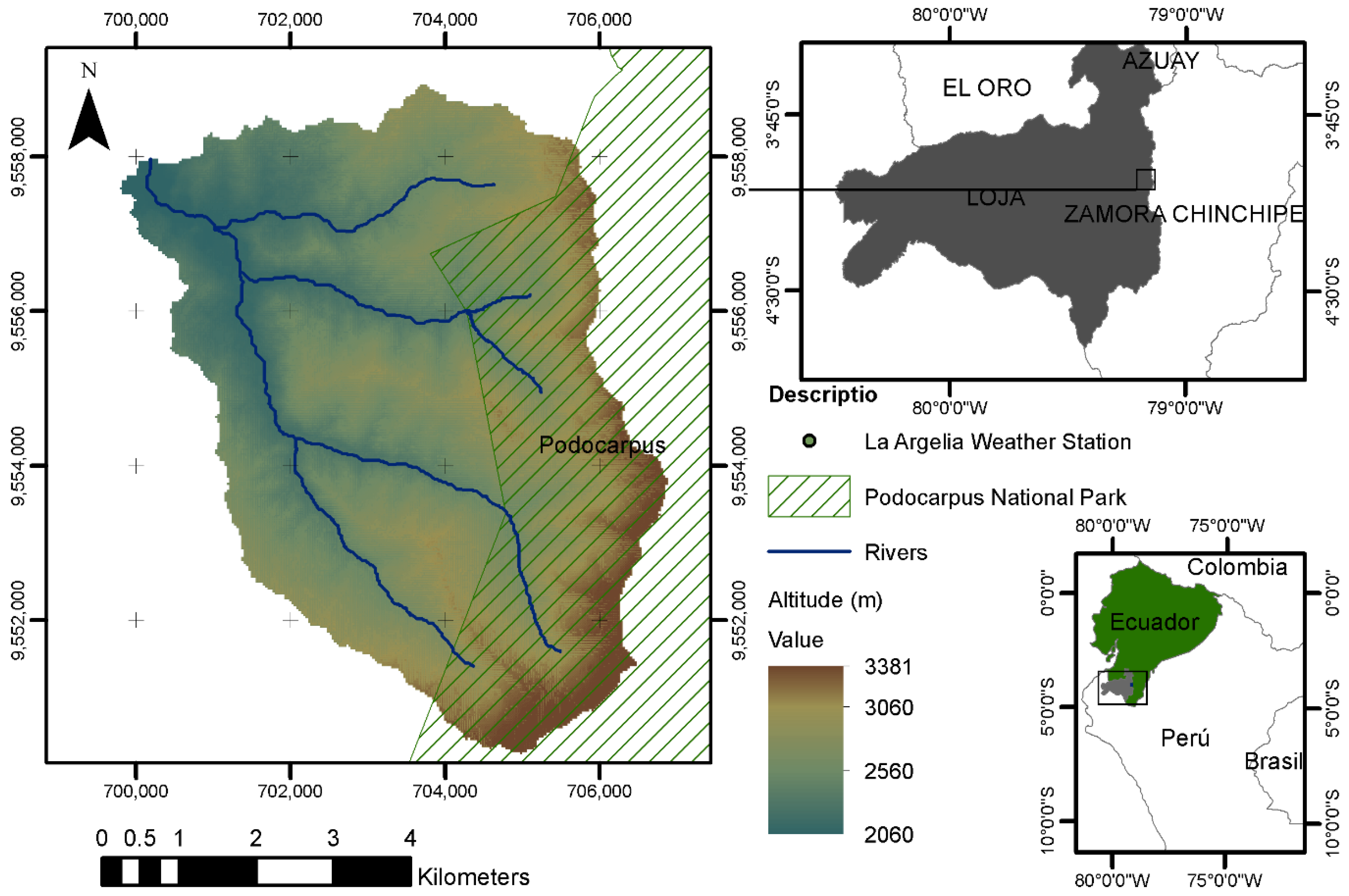
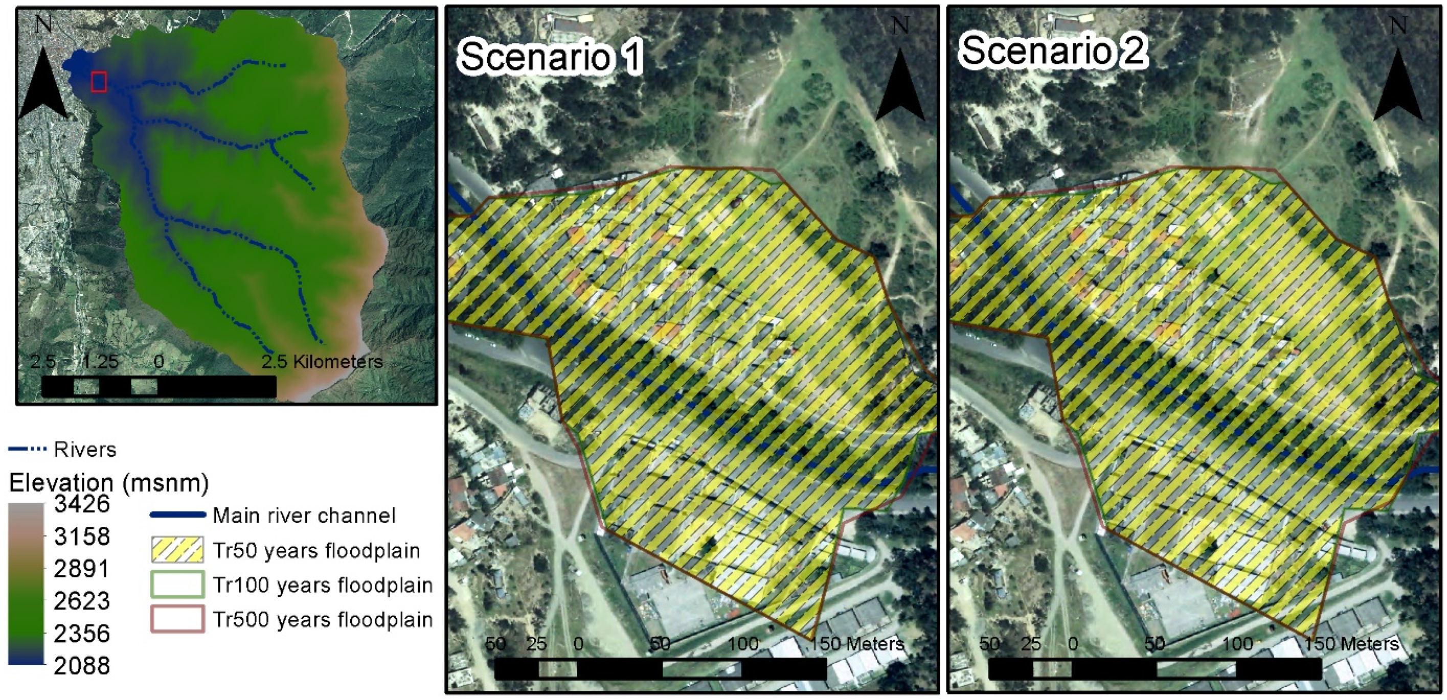
Article

Establishment of the Baseline for the IWRM in the Ecuadorian Andean Basins: Land Use Change, Water Recharge, Meteorological Forecast and Hydrological Modeling

by
Christian Mera-Parra
1,*,
Fernando Oñate-Valdivieso
1,2,
Priscilla Massa-Sánchez
1,3 and
Pablo Ochoa-Cueva
1,4
1
Master’s in Water Resources, Universidad Técnica Particular de Loja, San Cayetano Alto s/n, Loja 1101608, Ecuador
2
Department of Geology and Mine and Civil Engineering (DGMIC), Universidad Técnica Particular de Loja, San Cayetano Alto s/n, Loja 1101608, Ecuador
3
Department of Economics, Universidad Técnica Particular de Loja (UTPL), Loja 1101608, Ecuador
4
Department of Biological and Agricultural Sciences, Universidad Técnica Particular de Loja, San Cayetano Alto, Loja 110107, Ecuador
*
Author to whom correspondence should be addressed.
Submission received: 10 March 2021 / Revised: 28 April 2021 / Accepted: 8 May 2021 / Published: 12 May 2021

Abstract

:
This study was conducted in the Zamora Huayco (ZH) river basin, located in the inter-Andean region of southern Ecuador. The objective was to describe, through land use/land cover change (LUCC), the natural physical processes under current conditions and to project them to 2029. Moreover, temperature and precipitation forecasts were estimated to detail possible effects of climate change. Using remote sensing techniques, satellite images were processed to prepare a projection to 2029. Water recharge was estimated considering the effects of slope, groundcover, and soil texture. Flash floods were estimated using lumped models, concatenating the information to HEC RAS. Water availability was estimated with a semi-distributed hydrological model (SWAT). Precipitation and temperature data were forecasted using autoregressive and exponential smoothing models. Under the forecast, forest and shrub covers show a growth of 6.6%, water recharge projects an increase of 7.16%. Flood flows suffer a reduction of up to 16.54%, and the flow regime with a 90% of probability of exceedance is 1.85% (7.72 l/s) higher for 2029 than for the 2019 scenario, so an improvement in flow regulation is evident. Forecasts show an increase in average temperature of 0.11 °C and 15.63% in extreme rainfall by 2029. Therefore, intervention strategies in Andean basins should be supported by prospective studies that use these key variables of the system for an integrated management of water resources.

1. Introduction

Land use/land cover change (LUCC) impacts on various natural physical processes within watersheds have been extensively investigated worldwide [1,2]. The location of the Andean basins within intervention policies has also been the subject of analysis over the last several decades [3,4,5]. Changes and distribution of land use have an important influence on natural processes in a basin [1,2]. Water recharge, for example, shows sensitivity to different coverage due to the different infiltration rates that can occur under the same precipitation conditions [6,7], which is the reason why a change or alteration must be analyzed to evaluate its consequences. That is why water recharge was estimated in order to evaluate the effects that LUCC would have on it. In addition, the areas of the basin that favored it were spatially represented [8,9,10].
Another hydrological process that is influenced by LUCC are the flows associated with high intensity rains [11]; therefore, its analysis implies an element of judgment when making decisions at territorial level. The hydraulic simulation of flash floods was carried out to denote the impact of LUCC, generating information on flows and flood plains along the main channel [11] and giving technical support to the implementation of strategies associated with flood vulnerability reduction accompanied by land use planning policies and non-disruptive engineering practices [12].
Simulating the hydrological response of a basin under land use/land cover (LULC) scenarios is another key element for the integrated management of water resources [13], because it allows for the impact of LULC on the outlet flow of the basin [1,14,15]. This input is also the basis for the application of territorial policies and programs for the conservation of water sources.
Some studies have explored the relationship of LUCC with the hydrological response in basins. For example, for flow reproduction and calculation of sediment production in the Catamayo-Chira binational basin, the semi-distributed model called the Soil and Water Assessment Tool (SWAT) was implemented [16]. Similarly, the SWAT model was applied, obtaining satisfactory results at the Calumpang basin in Philippines [1].
In this study, the SWAT model is implemented for flow simulation, taking as scenarios: (a) a classified map of LULC in 2019, and (b) a projected map of LULC in 2029. With the generated hydrographs, flow duration curves (FDC) were prepared and the probability of exceedance of different flow values was analyzed for both scenarios.
Forecasted hydro-climatic information is scarce in the study region. In order to solve this need, the mean temperature and precipitation were forecasted through autoregressive and exponential smoothing models, widely used in annual series and meteorological variables [17,18,19,20]. Because these climatic data strongly influenced [21], their effects should be considered irreducible (even with the associated uncertainties), so intervention plans and adaptive strategies should be proposed to help mitigate these effects [22].
Our study focuses on the integrated water resources management (IWRM) in Andean basins. The ZH basin was used as a study case because of the interventions carried out there at the level of political institutions by decision-makers. Land use practices on the basin have been restricted in the last several years mainly due to municipal intervention policies for water sources preservation; a regional water fund operates in the area, ensuring that anthropogenic activities are not being carried out in areas considered as water recharge [23]. The basin has the also particularity of being located in a transition zone between a consolidated urban sector to a National Park [24].
The first results have been divided into two parts: this article, whose objective is to describe LUCC with some natural physical processes such as water recharge, flash floods, and water availability; temperature and precipitation forecasts have also been prepared to detail the possible effects of climate change to a horizon of 10 years. The second part is detailed in an article whose objective is to make a prospective analysis of water management in the ZH basin, including physical, socio-economic, and political-institutional variables, generating future scenarios and detailing strategies to reach a target horizon.

2. Materials and Methods

2.1. Study Area

The Zamora Huayco (ZH) river basin (3806 ha) is located in the inter-Andean region of the Loja province in southern Ecuador between the geographic coordinates 3°59′42″–4°04′03″ S and 79°11′54″–79°07′35″ W (Figure 1). The elevation of the basin ranges between 2120 and 3420 m asl, and its average slope is 0.65 m/m.
The basin’s climate is cold temperate mesothermal [25], characterized by an average annual temperature between 12 and 18 °C and average annual precipitation of 1047 mm. The wet season occurs from December to May and the dry season from June to November [26].
The basin has a predominantly forested vegetation. Since 1976, the forests of the basin have decreased by 19.3% [27]. The upper zone of the ZH basin is shared with the buffer zone of the Podocarpus National Park (PNP) [24]. Since the 1960s, natural vegetation near to PNP has been extensively removed to create pastures and farmland [27,28]. The main productive activities in the basin are agriculture and cattle raising [24,29]. In the ZH basin, there are two water catchments for potabilization that supply approximately 50% of the demand of the city of Loja with 450 l/s [30].

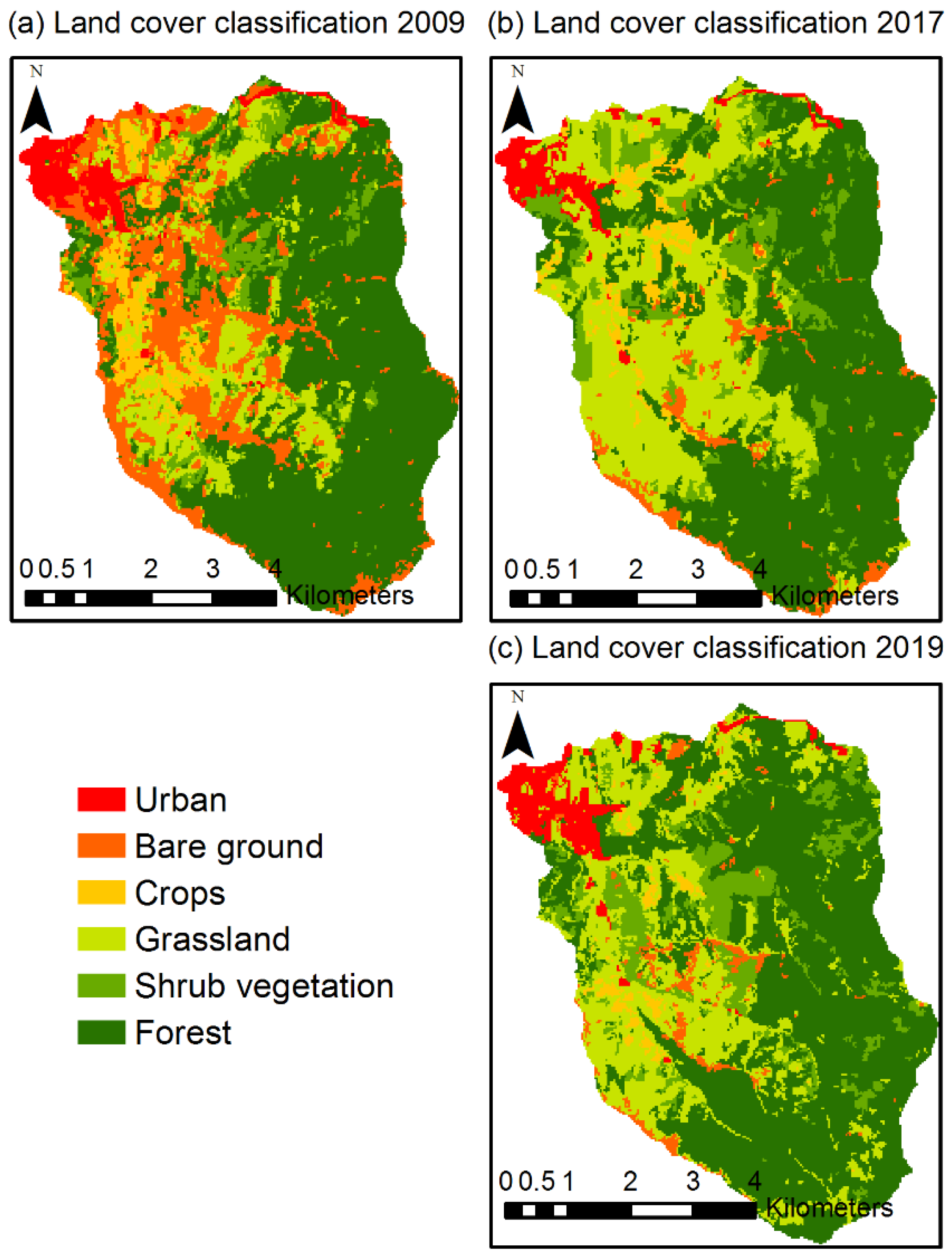
2.2. Land Use/Land Cover Change (LUCC)

Using remote sensing techniques, satellite images were processed to analyze LUCC. Three images were obtained: Landsat7 ETM (11 September 2009), Landsat8 OLI_TIRS (20 September 2017), and Sentinel 2B Level 1C (31 July 2019), which were ortho-rectified [31,32]. The satellite’s geometric coincidence with two temporarily invariable control points was verified, taking as reference an aerial photograph obtained from the SigTierras portal [33].
For the Landsat7 ETM and Landsat8 OLI_TIR images, the conversion to reflectance was performed to top of atmosphere (TOA) and to brightness temperature according to L. Congedo (2016). For the Sentinel 2B Level 1C image, the conversion was not performed as it is already scaled in TOA [32]. In the three images, the atmospheric correction Dark Object Subtraction (DOS) was performed [34]. In the three images, the topographic correction was also applied due to shading (CTS), using the Lambertian Cosine Model proposed by Teillet [35], for which it was necessary to determine the angle of incidence according to [36].
Radiometrically Terrain Corrected (RTC) data from DEM ALOS PALSAR, purchased from the Alaska Satellite Facility (ASF) Fairbanks, with a spatial resolution of 12.5 m, geocoded and radiometric corrected in its geographical extension [37], was used to carry out the CTS. LULC was obtained by supervised classification, using the method of the maximum likelihood classification algorithm based on Bayes’ theorem, of the three images previously processed. Three LULC categories of anthropogenic type and three of natural-physical type were classified.
For LUCC analysis, the procedure was analogous to that proposed by [38]. First, coverages obtained for the years 2009 and 2017 were analyzed; the quantitative change represented graphically in terms of gains and losses by categories was obtained.
As explanatory variables, maps were used showing the exchanges between the categories of grasslands and shrub vegetation, forest and bare soil, crops and grasslands, in addition to forest and crops. Additionally, a map containing the spatial trend of change was made, from forest to shrub vegetation, in order to generalize the pattern of change between these categories [39]. A ninth-degree polynomial order was considered.
Changes below 600 cells were ignored, in order to limit the transition model to 9 sub- transitions. The sub-transitions selected were: shrub vegetation to forest, bare soil to shrub vegetation, bare soil to grassland, bare soil to forest, grassland to shrub vegetation, grassland to forest, forest to shrub vegetation, forest to grassland, and grassland to crops.
The objective of the transition model is to create potential transition maps with a high degree of precision to execute the change model [38]. Transitions were grouped into a single sub-model; also, 6 explanatory variables were included.
The first explanatory variable was the shrub vegetation cover contained in the 2009 map. This model was included as a dynamic component that is recalculated over time during the course of the prediction. The other explanatory variables were included as static components, corresponding to the spatial trend maps and exchanges between categories previously generated.
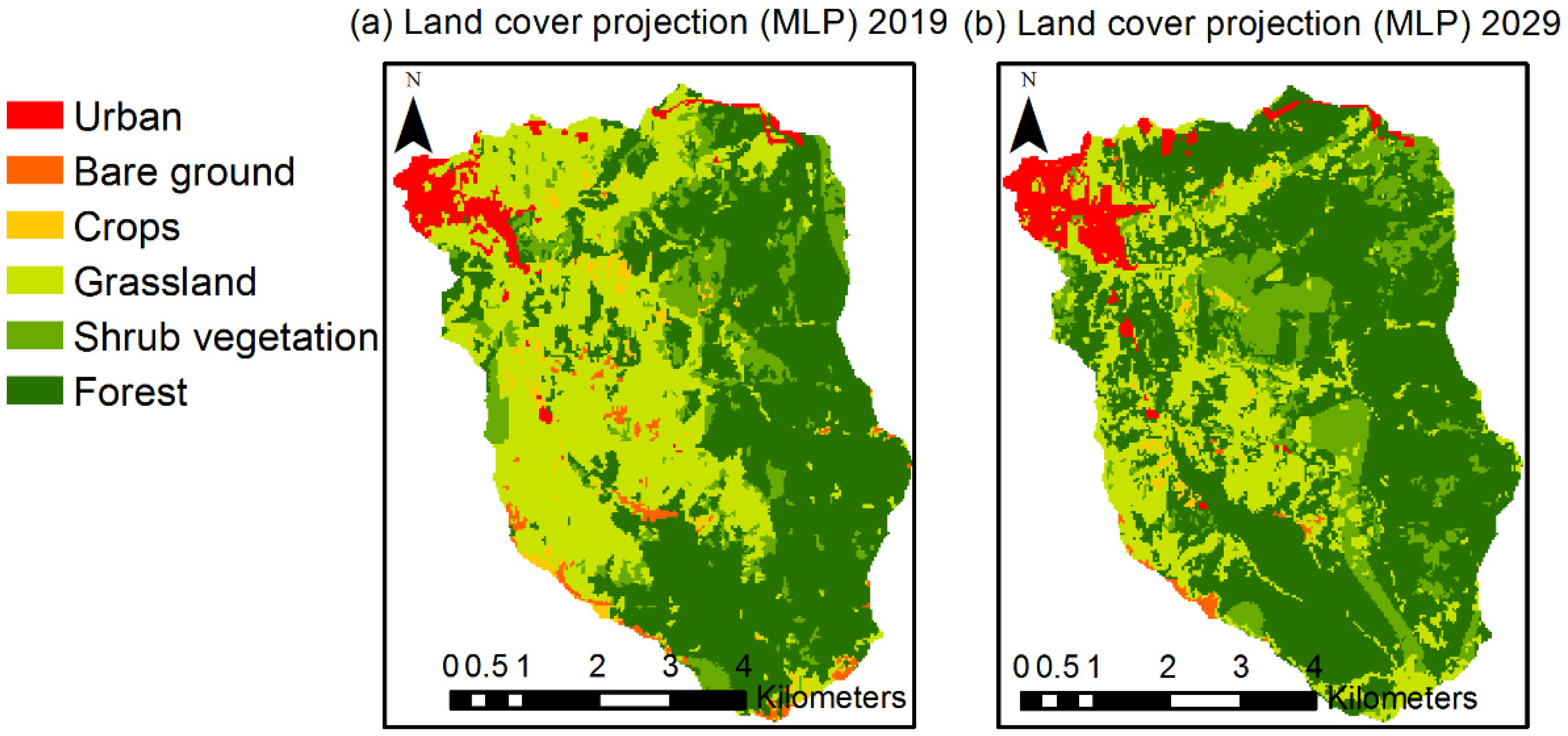
Physical restrictions of any kind have not been considered, because they are not necessary in a simple prediction [38]. For the transition model, the Multi-Layer Perceptron (MLP) algorithm has been applied, based on the Backpropagation (BP) algorithm, which is a supervised training algorithm [40]. For the change model, Markov chains were applied, generating a matrix with the probability that each category of land cover will change to any other category [38]. A validation was performed with the map generated for the year 2019.
To verify the image projected to 2019, a confusion matrix was performed and the kappa coefficient was determined. The confusion matrix shows the relationship between the reference data (2019 classified map) and the data to be evaluated (2019 projected map), constructing a matrix comparison of the classes verifying the overall accuracy of the projection by relating the number of points correctly assigned to the total [36]. The kappa coefficient evaluates the degree of agreement between categorical variables and takes into account the coincidences by randomness and by decision criteria; that is, it shows the degree of agreement that exists above random [41].
Similar to what was performed by [7,42], following the same conditions used in the 2009–2017 projection, the land use map for the year 2029 was generated, based on the 2009 and 2019 maps. The 2019 classified map containing LULC is called Scenario (1), and the 2029 projected map containing LULC is called Scenario (2).

2.3. Hydric Recharge Estimation

The multi-year average hydric recharge of the ZH basin was estimated, following the methodology set forth by [8] and also considering the infiltration criteria of [10], taking into account multi-year average precipitation, evapotranspiration (ET), basic soil infiltration rate, LULC, and terrain relief. The multi-year average rainfall was determined using data from La Argelia meteorological station over a 30-year period (1985 to 2015). Potential evapotranspiration ( E T P ) was determined through Hargreaves and Samani [43], who considered precipitation over the same time period (30 years).
As there is a correlation between the crop coefficient ( K c ) and the NDVI [44,45,46,47], K c was deducted by applying the expression [44]:
K c = 1.84   N D V I 2 1.03   N D V I + 0.42
NDVI was obtained from the Landsat8 OLI_TIRS image (20 September 2017). The multi-year average value of the calculated ETP was multiplied by the K c value to estimate the actual ET [48].
A slope map was generated using the DEM ALOS PALSAR RTC. This map was classified into 6 different categories (limits of <15, 15, 30, 50, 70, and >70%), assigning a coefficient to each. ( k p ) , known as the surface runoff coefficient, indicates the fraction that infiltrates due to the effect of slope [9]. Its value was taken from the table proposed by [8].
To each land use scenario (2019 and 2029) was assigned a value, named the land use coefficient ( k v ) , which represents the fraction that infiltrates due to the effect of the vegetation cover [9]. Its values were extracted from the table proposed by [8].
The infiltration fraction related to soil texture ( k f c ) was estimated using the following expression [10]:
k f c = 0.267 ln ( f c ) 0.000154 ( f c ) 0.723
where f c is the soil basic infiltration rate in mm/d. This was estimated using the Green-Ampt infiltration model [49], from soil data sampled in the ZH basin by [27].
According to [27], the most common soil texture in the study area is loam, with a bulk density from 0.07–1.09 g/cm³, organic carbon percentage from 1.66 to 5.98%, field capacity around 25.34%, and hydraulic conductivity that varies between 4.6 and 8.9 mm/h in a saturated state.
The multi-year average recharge, for LULC Scenarios (1) and (2), was determined using the following expression [8,10]:
R = ( P m a E T P · K c ) ( k p + k v + k f c )
where P m a is the multi-year average precipitation corresponding to the La Argelia station. E T P is the potential precipitation determined through Hargreaves and Samani.

2.4. Flash Flood Risk Assessment

Precipitation records of 51 years (from 1964 to 2015) were prepared and the data were controlled, corrected, and revised; the maximum precipitation in 24 h for each year was ordered. Different distribution functions were evaluated. Their precision was estimated through accumulated error, the Nash–Sutcliffe coefficient (NSE) and root mean square error (RMSE). Using GIS, physical parameters of the basin were determined such as area, average slope, channel length, channel slope, etc. Concentration time was estimated by Kirpich, Clark, and Temez [50,51].
For subsequent calculations, the concentration time was considered equal to design storm time. The maximum intensity was determined with this time, taking into account the intensity, duration, and frequency equations based on the maximum rainfall in 24 h corresponding to La Argelia station [52].
The hydrological response to extreme events was evaluated through synthetic unit hydrographs of the concentrated models Ven Te Chow, Snyder, Triangular SCS, and Temez. The mean and standard deviation of these results were calculated to assess dispersion and choose a model whose response is close to the mean. Curve numbers (CN) for scenario (1) and scenario (2) was determined using its respective land cover maps, taking into account the soil data provided by [27] through GIS.
Information corresponding to paths and flows was input to the HEC RAS hydraulic model and the outputs obtained were returned to GIS [11,53]. For the hydraulic evaluation, the main channel was divided into 29 cross sections. The roughness coefficients of the main channel and the banks were determined with the procedure explained by the USGS [54,55].

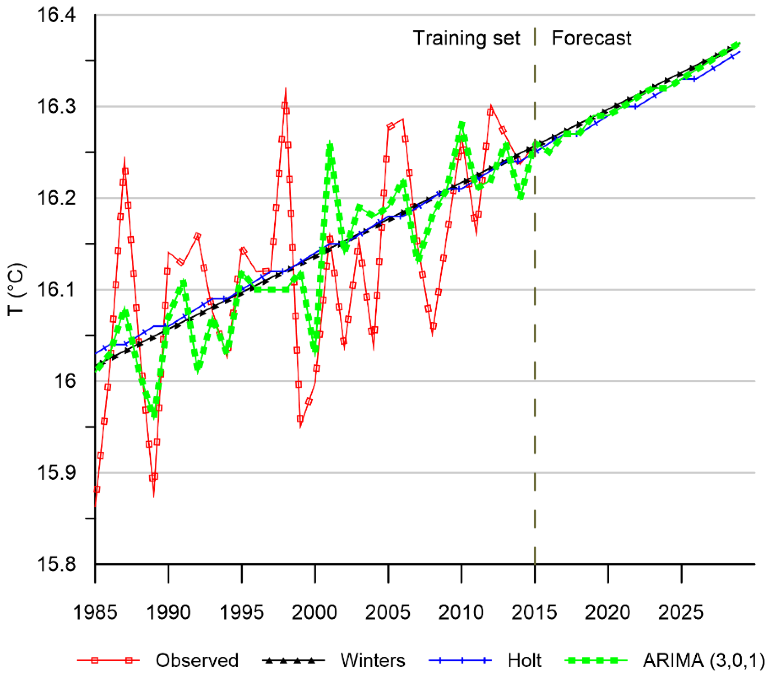
2.5. Meteorological Forecast

Meteorological information was taken from La Argelia station records, analogously to the method undertaken by [
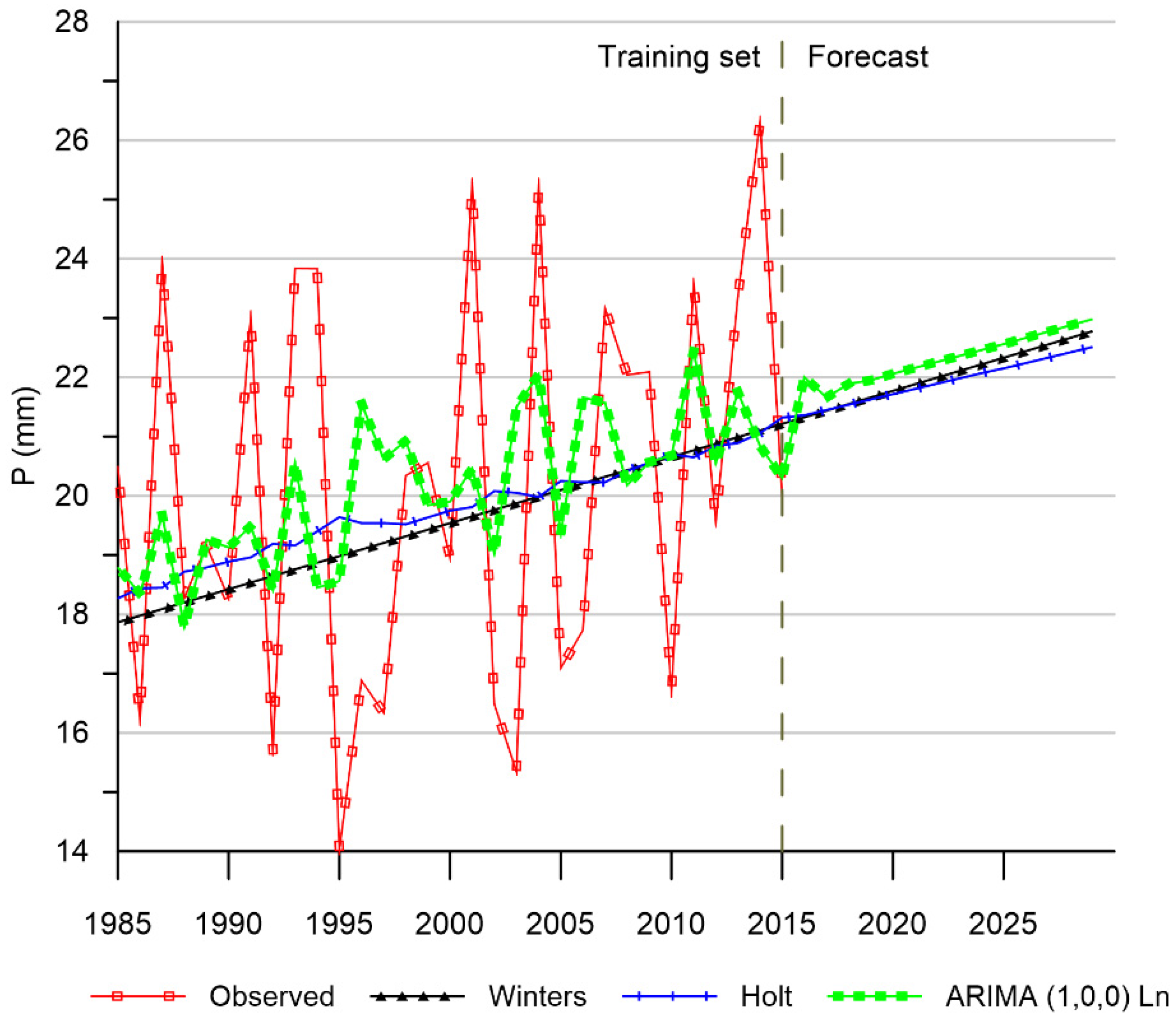
56]. It was developed with the annual mean temperature values; in addition, we obtained the values of maximum precipitation in 24 h of each month, and they were averaged obtaining an annual mean. These parameters will be referred to as T_average and Pmax_average from now on in the document.
The maximum precipitation data in 24 h of each month were prepared, since, as indicated by [21], one of the effects to a near horizon due to the increase of temperatures in high Andean basins is the increase in high intensity rainfall. These two annual series were forecast for the year 2029 using the Integrated Autoregressive Moving Average (ARIMA) model, the Holt exponential smoothing model (double exponent), and the Holt–Winters model (triple exponent). These models seek to describe the future behavior of the variables in relation to their past values [18].
The ARIMA model was used to predict series of a single variable. These are optimal with data series without seasonal variation, so they are widely used in annual series and meteorological variables [18,19,20]. In the ARIMA model (p, d, q), p indicates the correlation between current values and their immediate past values (autoregressive component), d indicates the order of differentiation to be applied in the series so that it becomes seasonal, and q indicates the moving average component order [17,18,57].
The double exponential model (Holt) considers an exponential smoothing, an estimation of trend, and a forecast. It involves adjusting the trend of the series at the end of each period. Triple Exponential Smoothing (Holt–Winters) adds an additional seasonality component to Holt model [58].
Series were attempted to be temporarily consistent, from 1985 to 2015. For the ARIMA model and the exponential smoothing models, their parameters were estimated (autoregressive components, seasonality, moving average and functional transformations), selecting the appropriate ones according to the best fit [17,19,56,57]. In order to verify the precision of the model and the chosen parameters, statistical measures such as the mean absolute error (MAE) and the root mean square error (RMSE) were determined.

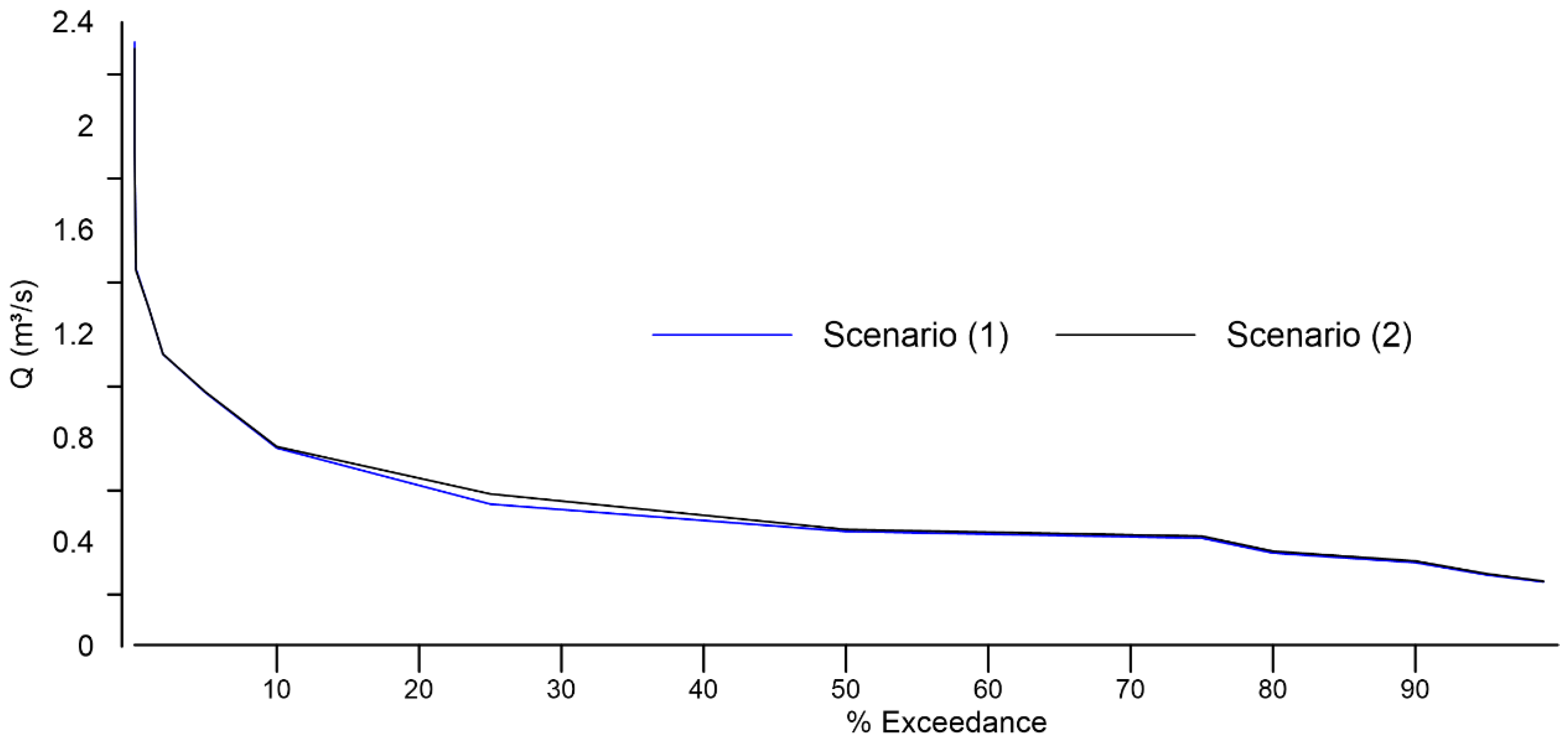
2.6. Water Availability Estimation

In order to estimate water availability, a semi-distributed hydrological modeling was carried out through SWAT, with LULC scenarios (1) and (2). With the flow values simulated, FDC were determined for each scenario. For the modelling, DEM ALOS PALSAR RTC was used and weather information was collected from La Argelia station. The model worked with 24 h precipitation and daily average values of maximum temperature, minimum temperature, relative humidity, and wind speed. Solar radiation was estimated applying the Hargreaves and Samani equations [43].
Monthly climatic parameters required by SWAT were calculated using the SWAT Weather Database tool [59], similar to what was done by [14]. Missing values were input as −99.0, so that SWAT can estimate data for that day [60]. A soil map was generated from the soil sampling data provided by [27], data was supplemented and adapted to SWAT requirements, and the K U S L E variable was determined by applying Williams equations [60]. As these are soils with unique characteristics, they were added to the SWAT user-soil database table, analogously to the research carried out by [61].
The LULC maps of 2019 and 2029 contained in scenarios (1) and (2) respectively were used for analysis. Coverages of forest, shrub vegetation, grassland, bare soil, agriculture, and urban life were concatenated to SWAT database coverages considering similarity between characteristics and parameters, similar to what was done by [16].
The slopes range considered for the definition of the hydrological response units (HRU) were selected based on those established by [8], which respond to an adaptation of the considerations made by [9] considering water infiltration easiness into the ground due to slope, similar to what was performed by [62].
Simulation was performed considering a daily periodicity. The number of years of omission (NYSKIP) was entered, which is necessary to train the model; in this case 5 years was input as NYSKIP. As a general rule, a minimum of 3 NYSKIP is an acceptable heating period [
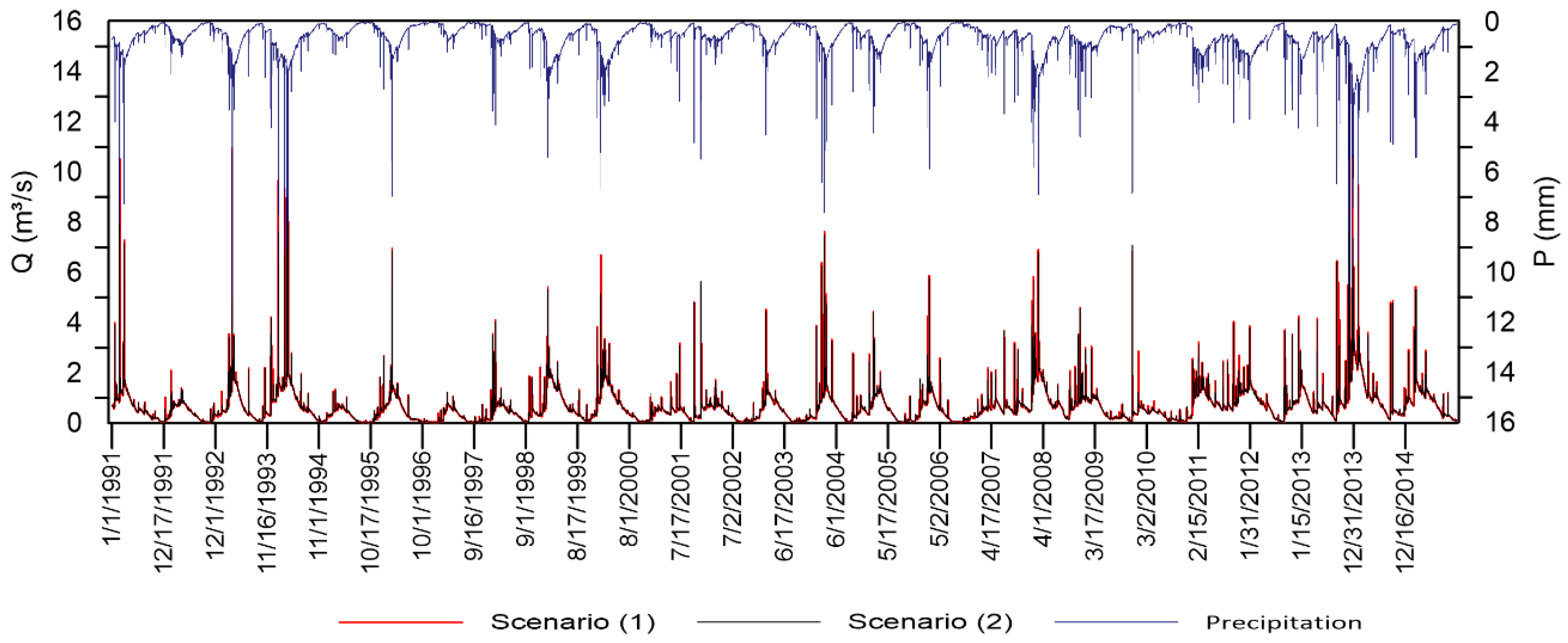
1]. The simulated flow begins in 1991 and ends in 2015.
In order to analyze the occurrence and frequency of the flow at the exit of the basin, and to be able to predict its availability, FDC were generated for each scenario [63,64]. This theoretical curve has been determined from modeled daily average data.

3. Results

3.1. LULC and LUCC

First, when analyzing the gains and losses by categories, it was evident that the most important changes between 2009 and 2017 occurred in relation to forest and grassland cover. When analyzing these categories individually, in the forest cover the most significant exchanges occurred with the categories of shrub vegetation, bare soil, and crops; for grassland cover, the categories with the most important exchanges were crops and shrub vegetation.
It is for this reason that the explanatory variables, and the projection’s transition model to year 2019 based on the years 2009 and 2017, included maps with exchanges between categories of grasslands and shrub vegetation, forest and bare soil, crops and grasslands, in addition to forest and crops. Moreover, because of the evident pattern of change between forest and shrub vegetation, this was included in the transition model as a map of spatial trend of change.
The spatial trend of change map was generated with a ninth-degree polynomial order, because lower polynomial orders do not significantly influence the projection. In addition, with a ninth-degree polynomial order, a higher value was reached in the confusion matrix overall accuracy. This map showed greater sensitivity within the transition model.
The transition model used for the projection to 2019 reached an accuracy rate of 78.47% (2009–2017) after being executed with the MLP algorithm and under a threshold of 10,000 iterations. An accuracy rate of about 80% is acceptable [65]. Nevertheless, other investigations support using a transition model with an accuracy rate greater than 70% for land cover prediction [38,66]. The confusion matrix, having as a reference parameter the supervised classification for 2019 and its projected data; delivered an overall accuracy of 77.03%, close to the value obtained [1].
The kappa index, analogously to the confusion matrix, provided an overall value of 0.6813. According to [67], it has a moderate concordance; for [68], it holds a substantial precision evaluation; for [69], it is considered a fair-to-good concordance; and for [70], it has a degree of agreement that is close to very good; this interpretive scale is detailed by [41]. Based on [41], the projection is considered acceptable.
Under the same conditions used in the 2019 projections with the maps of the years 2009 and 2017, the land use map for the year 2029 was generated, based on the classified maps of the years 2009 and 2019. Applying the MLP algorithm and under a 10,000 iterations threshold, an accuracy rate of 73.76% was achieved in the transition model of the map projected to 2029. Land cover classified maps for (a) 2009, (b) 2017, and (c) 2019 are presented in Figure 2. Figure 3 shows the projected maps (MLP) for (a) 2019 and (b) 2029.
Map (c) in Figure 2 represents LULC of scenario (1); map (b) in Figure 3 contains LULC of scenario (2). When analyzing the coverage extension, it is evident that the forest area is the most abundant, occupying in the basin 54.81% of its total extension for the year 2019, while on projection for 2029 it occupies 58.72%, so an increase of 3.91% is evident. Another coverage that shows an increase is shrub vegetation, occupying in 2019 an extension of 11.02%, and in the projection for 2029 of 13.71%, denoting an increase of 2.69%. Forest and shrub covers have a projected growth of 6.6%.
Bare soil, grasslands, and crop coverages have presented a reduction of 2.35%, 3.27%, and 0.99% respectively in their projection to 2029, in relation to 2019. Urban extension coverage has not shown changes. These results are presented in Table 1.

3.2. Hydric Recharge Analysis

Multi-year average precipitation obtained for the period under analysis is 1047.8 mm. ETP was equal to 1173.88 mm. The average K c coefficient of the basin is 0.293. Based on these, the multi-year average recharge estimated for 2019 in the basin is 614.05 mm; for 2029 it is 618.45 mm. This increase is associated with forest and shrub vegetation cover gain. It has also been determined that the highest recharge values are above the 2350 m asl level. This area has mostly forest and shrub vegetation cover. The soil is loam texture mostly, and in some areas, there are also high values of infiltration rates (>16 mm/h). Spatial distribution of hydric recharge results in the basin is presented in Figure 4.

3.3. Floodplains

A series of maximum precipitation in 24 h of each year was evaluated with different distribution functions using spreadsheets provided by [71]. Precision was estimated through accumulated error, the Nash–Sutcliffe coefficient (NSE), and root mean square error (RMSE). These results are detailed in Table 2.
Gamma of 2 parameters was established as the distribution function that best fits the data series. Using this function, the maximum precipitation in 24 h for 3 return periods (Tr) (50, 100, and 500 years) were determined.
Using LULC maps and soil sampling data provided by [27], CN was determined, being 61.66 and 60.96 for the years 2019 and 2029 respectively. There is a projected decrease to the year 2029 due to the increase in shrub and forest vegetation.
Concentration times estimated by the equations provided by Kirpich, Clark, and Temez were 0.53, 1.46, and 2.71 h respectively. Temez was chosen because it adjusts better with the morphological and high Andean conditions of the ZH basin [72].
After calculating mean and standard deviation of peak flow rates obtained with synthetic unit hydrographs, it was determined that the model with results closest to the mean is the Ven Te Chow, which was therefore selected to determine the flood flow rates. Table 3 summarizes obtained values.
The channel was divided into 29 cross sections. The roughness coefficients of the main channel and banks were 0.04 and 0.07 (s/m1/3) respectively. Table 4 details a summary of the hydraulic results, the floodplains, and areas susceptible to flooding.

3.4. Meteorological Forecast

Statistical measures such as MAE, RMSE, and R2 were determined to verify the model’s precision and the chosen parameters. For T average, adjustment statistics are presented in Table 5, and for Pmax average in Table 6. According to the obtained results, forecast Pmax average precision is lower compared to that obtained for T average.
In Figure 5, the ARIMA (3,0,1) model and exponential smoothing models are closely similar, both indicating an 0.11 °C increase in the average temperature for the year 2029.
In Figure 6, models keep similarities in forecasts, but given the stochastic nature of rainfall [73], they do not reach a high adjustment value. Models show an increasing trend, according to the ARIMA model (1,0,0), toward an increase of 15.63% in the year 2029, taking the year 2015 as a reference. In contrast, other researchers point out that in high Andean zones of Ecuador there is an incremental tendency in annual rainfall [74].
The temperature increase in Figure 5 is related to the increase in precipitation in Figure 6. Temperature peaks precede the precipitation peaks and when the precipitation presents higher values the temperature shows a decrease with a convex curve. In the future, as temperature increases, the peaks of precipitation would also increase, resulting in storms of greater intensity and therefore an increased risk of extreme hydrological events such as floods.
In Figure 5 and Figure 6, the forecast final values are close to each other. After the training set, those have an upward growth, following the series’ central tendency. This is because the ARIMA model and the exponential smoothing models are adjusting to series that have no periodicity.

3.5. Basin Hydrological Response

Simulated hydrographs show a seasonality associated with 24 h precipitation. The 2019 scenario reaches higher values in peak flows and lower values during dry season. The scenario for 2029 shows better flow regulation by obtaining lower values at peak flows and higher in the dry season in relation to the 2019 scenario. The hydrological response of the basin is shown in Figure 7.
Surface runoff (annual average) decreased by 1.37%, due to the increase in forest and shrub vegetation areas and the decrease in agricultural cover. The flow duration curves (FDC) (Figure 8) show that, for the 2019 coverage scenario, there is a flow of 0.3228 m3/s with a 90% probability of exceedance, while for the 2029 scenario it is 0.328 m3/s. The flow regime with a 90% probability of exceedance is 1.85% (7.72 l/s) higher for the 2029 than it is for the 2019. This trend has found up to a 1% probability of exceedance, reaching an increase of 1.05%.
On the other hand, with a probability of exceedance of 0.01%, the 2019 coverage scenario has a flow of 2323 m3/s. For the 2029 scenario, it is 2298 m3/s; that is, there is a decrease of 1.07%, a trend that is maintained for exceedance probabilities of less than 1%. These results are related to the behavior of extreme flood events flows analyzed in Section 4.3.

4. Discussion

4.1. LULC and LUCC Analysis

Land use practices such as agriculture and livestock have been limited in recent years mainly due to municipal intervention policies for the preservation of water sources. Actions taken have allowed a forest recovery, which is evidenced in the projected increase in its coverage. Additionally, [75] indicates that the population of the area will decrease at a rate greater than 1.56%, which makes sense with the non-existent growth of urban cover.

4.2. Hydric Recharge Analysis

Forest and shrub vegetation cover gain increases hydric recharge rate since it supposes a greater fraction of rain that is intercepted by vegetation. Areas where this increase is greater are located above 2350 m asl, which is also the level where a catchwater is located.
All areas related to water supply are protected by a mercantile escrow subscribed to by local government and the Regional Water Fund FORAGUA. One of FORAGUA’s main activities is the purchase of lands that are located within zones identified as water recharge zones (WRA). Most of the purchased land was declared as a municipal reserve. In those zones, any exploitation is forbidden [23]. That is why forest species have the potential to extend their borders and improve the water regulation in the basin.

4.3. Floodplains Analysis

According to Table 4 and Figure 9, floodplain margins and flooding-susceptible areas have a limited increase for return periods greater than 50 years. In addition, a reduction is expected by 2029. A remarkable number of rural buildings, agricultural land, and orchards are located on the riverside within the margin of the floodplains. This problem occurs because of fertility and ease of access to the areas.

4.4. Meteorological Forecast Analysis

Average temperature increments indicate an increase in terrestrial radiation (reflected solar) due to the presence of clouds (mainly before the first hours of radiation) and greenhouse gases (GHG) [76,77].
Adaptations in the basin, due to climate change, should be channeled around the increase in average temperature and the increase in high intensity rainfall. Being temperature linked to atmospheric pressure and amount of water vapor in the air, as it increases, the air rises by convection and gets colder, producing cloudiness, and eventually precipitation [76,77]. As there is an increasing trend in maximum precipitation, there is a probable increase in peak flow rates of flash floods.
Forecasts show a tendency to increase in maximum rainfall in 24 h, so a scenario considering its possible effects is appropriate to achieve assertive management of hydrological risks [22].
Precipitation forecasts do not provide reliable estimations of future patterns at the local scale. However, they point to an increasing trend. [22] also reports uncertainties in the precipitation forecast, noting that these are only worthy when the impacts of climate change are considered in their scenarios.

4.5. Basin Hydrological Response Analysis

FDC comparison shows an improvement on the water regulation capacity. Forest and shrub vegetation cover increments influenced the surface runoff and water recharge, and therefore the flow regulation. The greatest contribution to base flow was caused by lateral and underground flows. According to the model, the annual average of both contributions to the base flow in the 2019 scenario was 455.35 mm, while for the 2029 scenario it was 459.67 mm. These results support the premise that a mainly wooded area limits the source material of surface runoff, and therefore favors water recharge [78]. Forest and shrub vegetation trap sediment and delay runoff between adjacent zones, facilitating percolation and drainage of water through the soil, increasing base flow [1,78].

4.6. Actual Context of the ZH Basin and the Need for IWRM

These particular models comply with the initial stage of IWRM diagnosis. In a complementary investigation, these results are expected to be used in a prospective study of future scenarios and to develop a strategic plan to achieve a desired future, particularly by developing territorial prospective and implementation strategy stages [3]. A detailed description of each model used is given in Table S1 in Supplementary Materials.
In addition, the management of this particular basin is of vital importance for Loja city due to the fact that it provides about 50% of the water for human consumption [30] not considering its agricultural use, so, there is demographic pressure around the hydric resource [79]. The basin has been intervened with in terms of conservation, with highly restrictive regulations related to human activities. The local government has also bought lands closed to catchments to protect water supply, however, wealthy owners still retain some properties focused on areas in the upper part of the basin [80]; therefore, the conditions of change of use and land cover are atypical and deserve to be studied, in addition to their effect on the different natural physical processes associated with water. The meteorological forecast was developed in order to contextualize the increase in temperature and extreme rainfall and to raise the need for adaptation measures to climate change.

5. Conclusions

Forest and shrub covers show an increase for the 2029 scenario, which has a strong influence on natural physical processes in the basin. Hydric recharge suggests an increase in 2029, with the areas that favor it mostly located above 2350 m asl. The drinking water catchment points above this altitude, so it must be ensured that agricultural practices be carried out below this level in the basin.
Peak flow rates of flash floods show a reduction for the future LULC scenario. Flood margins do not show a significant decrease; however, on average they are located 36 m from the course of the river, so agricultural practices and human settlements should be limited to outside that margin to decrease their vulnerability.
Forecasts made up with the three models considered (Holt, Winters, and ARIMA) show an increase in average temperature and extreme rainfall (even with the associated uncertainties). On this issue, management strategies must deal with unpredictability and a correct capacity to respond to possible conditions of climate change.
Considering that the flow regime with a 90% probability of exceedance is greater for scenario (2) than for scenario (1), it is evident that basin recovery is due to an improvement on flow regulation related to increase of forest and shrub vegetation cover.
Intervention strategies in Andean basins can be supported in prospective studies using these key system variables focused on the integrated management of water resources.

Supplementary Materials

The following is available online at https://0-www-mdpi-com.brum.beds.ac.uk/article/10.3390/land10050513/s1. Table S1: Description of each methodology subsection, data, and models used.

Author Contributions

Conceptualization, P.M.-S.; Data curation, C.M.-P. and P.O.-C.; Formal analysis, C.M.-P.; Investigation, C.M.-P.; Methodology, C.M.-P. and F.O.-V.; Project administration, P.M.-S.; Software, C.M.-P.; Supervision, F.O.-V. and P.M.-S.; Validation, F.O.-V.; Visualization, P.M.-S.; Writing—original draft, C.M.-P.; Writing—review & editing, P.O.-C. All authors have read and agreed to the published version of the manuscript.

Funding

This research did not receive any specific grant from funding agencies in the public, commercial, or not-for-profit sectors. The APC was funded by the Universidad Técnica Particular de Loja—Ecuador.

Institutional Review Board Statement

Not applicable.

Informed Consent Statement

Not applicable.

Data Availability Statement

Some or all data and models that support the findings of this study are available from the corresponding author upon reasonable request.

Acknowledgments

The authors would like to thank the “Instituto Nacional de Meteorología e Hidrología del Ecuador” (INAMHI) for facilitating the climate data. Special thanks to all professors of the Master’s degree in Hydrological Resources from the Universidad Técnica Particular de Loja (UTPL) for their support.

Conflicts of Interest

The authors declare no conflict of interest.

References

  1. Boongaling, C.G.K.; Faustino-Eslava, D.V.; Lansigan, F.P. Modeling land use change impacts on hydrology and the use of landscape metrics as tools for watershed management: The case of an ungauged catchment in the Philippines. Land Use Policy 2018, 72, 116–128. [Google Scholar] [CrossRef]
  2. Ewunetu, A.; Simane, B.; Teferi, E.; Zaitchik, B.F. Land cover change in the blue nile river headwaters: Farmers’ perceptions, pressures, and satellite-based mapping. Land 2021, 10, 68. [Google Scholar] [CrossRef]
  3. Manzano, L.R.; Díaz, C.; Gómez, M.A.; Mastachi, C.A.; Soares, D. Use of structural systems analysis for the integrated water resources management in the Nenetzingo river watershed, Mexico. Land Use Policy 2019, 87, 2–11. [Google Scholar] [CrossRef]
  4. Baude, M.; Meyer, B.C.; Schindewolf, M. Land use change in an agricultural landscape causing degradation of soil based ecosystem services. Sci. Total Environ. 2019, 659, 1526–1536. [Google Scholar] [CrossRef] [PubMed]
  5. Delgado, A.M.; Pantoja, F. Structural analysis for the identification of key variables in the Ruta del Oro, Nariño Colombia. Dyna 2015, 82, 27–33. [Google Scholar] [CrossRef]
  6. Edwards, E.C.; Harter, T.; Fogg, G.E.; Washburn, B.; Hamad, H. Assessing the effectiveness of drywells as tools for stormwater management and aquifer recharge and their groundwater contamination potential. J. Hydrol. 2016, 539, 539–553. [Google Scholar] [CrossRef] [Green Version]
  7. Guerrero-Morales, J.; Fonseca, C.R.; Goméz-Albores, M.A.; Sampedro-Rosas, M.L.; Silva-Gómez, S.E. Proportional Variation of Potential Groundwater Recharge as a Result of Climate Change and Land-Use: A Study Case in Mexico. Land 2020, 9, 364. [Google Scholar] [CrossRef]
  8. Junker, M. Método RAS Para Determinar la Recarga de Agua Subterránea; Forgaes: San Salvador, El Salvador, 2005. [Google Scholar]
  9. Schosinsky, G.; Losilla, M. Modelo analítico para determinar la infiltración con base en la lluvia mensual. Rev. Geológica América Cent. 2000, 23, 43–55. [Google Scholar] [CrossRef]
  10. Schosinsky, G. Cálculo de la recarga potencial de acuíferos mediane un balance hídrico de suelos. Rev. Geológica América Cent. 2006, 34–35, 13–30. [Google Scholar]
  11. Golshan, M.; Jahanshahi, A.; Afzali, A. Flood hazard zoning using HEC-RAS in GIS environment and impact of manning roughness coefficient changes on flood zones in Semi-arid climate. Desert 2016, 21, 24–34. [Google Scholar] [CrossRef]
  12. Liu, J.; Shi, Z. wu Quantifying land-use change impacts on the dynamic evolution of flood vulnerability. Land Use Policy 2017, 65, 198–210. [Google Scholar] [CrossRef]
  13. Arteaga, J.; Ochoa, P.; Fries, A.; Boll, J. Identification of Priority Areas for Integrated Management of Semiarid Watersheds in the Ecuadorian Andes. JAWRA J. Am. Water Resour. Assoc. 2020, 56, 270–282. [Google Scholar] [CrossRef]
  14. Mararakanye, N.; Le Roux, J.J.; Franke, A.C. Using satellite-based weather data as input to SWAT in a data poor catchment. Phys. Chem. Earth 2020, 117, 102871. [Google Scholar] [CrossRef]
  15. Wilson, T.S.; Van Schmidt, N.D.; Langridge, R. Land-use change and future water demand in California’s Central Coast. Land 2020, 9, 322. [Google Scholar] [CrossRef]
  16. Oñate-Valdivieso, F.; Bosque Sendra, J. Semidistributed hydrological model with scarce information: Application to a large south american binational basin. J. Hydrol. Eng. 2014, 19, 1006–1014. [Google Scholar] [CrossRef]
  17. Aguado-Rodríguez, G.J.; Quevedo-Nolasco, A.; Castro-Popoca, M.; Arteaga-Ramírez, R.; Vázquez-Peña, M.A.; Zamora-Morales, B.P. Meteorological variables prediction through ARIMA models. Agrociencia 2016, 50, 1–13. [Google Scholar]
  18. Hossain, M.; Hasan, E.; Alauddin, M. The Variability of the Historical and Future Temperature in Bangladesh. Br. J. Appl. Sci. Technol. 2017, 20, 1–13. [Google Scholar] [CrossRef]
  19. Norouzi, M. Time Series Analysis on the Appropriate Time for Malaria Residual Spraying Based on Anopheles abundance, Temperature, and Precipitation between 2009–2016 in Kazerun, South of Iran. J. Health Sci. Surveill. Syst. 2018, 6, 99–105. [Google Scholar]
  20. Rodrigues, J.; Deshpande, A. Prediction of Rainfall for all the States of India Using Auto-Regressive Integrated Moving Average Model and Multiple Linear Regression. In Proceedings of the International Conference on Computing, Communication, Control and Automation, Pune, India, 17–18 August 2017; pp. 1–4. [Google Scholar] [CrossRef]
  21. Mora, D.E.; Campozano, L.; Cisneros, F.; Wyseure, G.; Willems, P. Climate changes of hydrometeorological and hydrological extremes in the Paute basin, Ecuadorean Andes. Hydrol. Earth Syst. Sci. 2014, 18, 631–648. [Google Scholar] [CrossRef] [Green Version]
  22. Buytaert, W.; Vuille, M.; Dewulf, A.; Urrutia, R.; Karmalkar, A.; Célleri, R. Uncertainties in climate change projections and regional downscaling in the tropical Andes: Implications for water resources management. Hydrol. Earth Syst. Sci. 2010, 14, 1247–1258. [Google Scholar] [CrossRef] [Green Version]
  23. Foragua Mecanismo Financiero FORAGUA. Available online: http://www.foragua.org/ (accessed on 29 April 2020).
  24. Mejía-Veintimilla, D.; Ochoa-Cueva, P.; Samaniego-Rojas, N.; Félix, R.; Arteaga, J.; Crespo, P.; Oñate-Valdivieso, F.; Fries, A. River Discharge Simulation in the High Andes of Southern Ecuador Using High-Resolution Radar Observations and Meteorological Station Data. Remote Sens. 2019, 11, 2804. [Google Scholar] [CrossRef] [Green Version]
  25. INAMHI Tipo de Climas. Available online: http://www.serviciometeorologico.gob.ec/geoinformacion-hidrometeorologica/ (accessed on 30 April 2020).
  26. Oñate-Valdivieso, F.; Uchuari, V.; Oñate-Paladines, A. Large-Scale Climate Variability Patterns and Drought: A Case of Study in South-America. Water Resour. Manag. 2020, 34, 2061–2079. [Google Scholar] [CrossRef]
  27. Ochoa-Cueva, P.; Fries, A.; Montesinos, P.; Rodríguez-Díaz, J.A.; Boll, J. Spatial Estimation of Soil Erosion Risk by Land-cover Change in the Andes OF Southern Ecuador. Land Degrad. Dev. 2015, 26, 565–573. [Google Scholar] [CrossRef]
  28. González-Jaramillo, V.; Fries, A.; Zeilinger, J.; Homeier, J.; Paladines-Benitez, J.; Bendix, J. Estimation of Above Ground Biomass in a Tropical Mountain Forest in Southern Ecuador Using Airborne LiDAR Data. Remote Sens. 2018, 10, 660. [Google Scholar] [CrossRef] [Green Version]
  29. Zarate, C. Hacia un Modelo de Ordenación Para los Territorios de Protección Natural del Área de Influencia Inmediata de la Ciudad de Loja. Microcuenca El Carmen; Universidad de Cuenca: Cuenca, Ecuador, 2011. [Google Scholar]
  30. Alvarez Bustamante, L. Disponibilidad y Demanda del Recurso Hídrico Superficial; Estudio de caso: Subcuenca Zamora Huayco, Ecuador, 2017. [Google Scholar]
  31. Hansen, M.C.; Loveland, T.R. A review of large area monitoring of land cover change using Landsat data. Remote Sens. Environ. 2012, 122, 66–74. [Google Scholar] [CrossRef]
  32. Pandžić, M.; Mihajlović, D.; Pandžić, J.; Pfeifer, N. Assessment of the geometric quality of sentinel-2 data. Int. Arch. Photogramm. Remote Sens. Spat. Inf. Sci. ISPRS Arch. 2016, 41, 489–494. [Google Scholar] [CrossRef] [Green Version]
  33. MAGAP Ortofoto. Available online: http://mapas.sigtierras.gob.ec/ortofoto/ (accessed on 1 March 2020).
  34. Congedo, L. Semi-Automatic Classification Plugin Documentation. Release 2016, 5, 268. [Google Scholar] [CrossRef]
  35. Fang, Y.; Zhao, J.; Liu, L.; Wang, J. Comparision of Eight Topographic Correction Algorithms Applied to Landsat-8 OLI Imagery Based on the DEM. In Proceedings of the IOP Conference Series: Earth and Environmental Science, Prague, Czech Republic, 7–11 September 2020; Volume 428. [Google Scholar] [CrossRef] [Green Version]
  36. Chuvieco, E. Teledetección Ambiental: La Observación de la Tierra Desde el Espacio; Tercera; Ariel Ciencia: Barcelona, Spain, 2007; ISBN 84-344-8047-6. [Google Scholar]
  37. Alaska Satellite Facility ALOS PALSAR Terrain-Corrected (RTC) DEM data. Available online: https://search.asf.alaska.edu/ (accessed on 14 May 2020).
  38. Mishra, V.; Rai, P.; Mohan, K. Prediction of land use changes based on land change modeler (LCM) using remote sensing: A case study of Muzaffarpur (Bihar), India. J. Geogr. Inst. Jovan Cvijic SASA 2014, 64, 111–127. [Google Scholar] [CrossRef]
  39. Hamdy, O.; Zhao, S.; Salheen, M.A.; Eid, Y.Y. Analyses the Driving Forces for Urban Growth by Using IDRISI®Selva Models Abouelreesh-Aswan as a Case Study. Int. J. Eng. Technol. 2017, 9, 226–232. [Google Scholar] [CrossRef] [Green Version]
  40. Khoi, D.D.; Murayama, Y. Forecasting areas vulnerable to forest conversion in the tam Dao National Park region, Vietnam. Remote Sens. 2010, 2, 1249–1272. [Google Scholar] [CrossRef] [Green Version]
  41. Foody, G.M. Explaining the unsuitability of the kappa coefficient in the assessment and comparison of the accuracy of thematic maps obtained by image classification. Remote Sens. Environ. 2020, 239, 111630. [Google Scholar] [CrossRef]
  42. Oñate-Valdivieso, F.; Bosque Sendra, J. Application of GIS and remote sensing techniques in generation of land use scenarios for hydrological modeling. J. Hydrol. 2010, 395, 256–263. [Google Scholar] [CrossRef]
  43. Zanetti, S.S.; Dohler, R.E.; Cecílio, R.A.; Pezzopane, J.E.M.; Xavier, A.C. Proposal for the use of daily thermal amplitude for the calibration of the Hargreaves-Samani equation. J. Hydrol. 2019, 571, 193–201. [Google Scholar] [CrossRef]
  44. Alam, M.S.; Lamb, D.W.; Rahman, M.M. A refined method for rapidly determining the relationship between canopy NDVI and the pasture evapotranspiration coefficient. Comput. Electron. Agric. 2018, 147, 12–17. [Google Scholar] [CrossRef]
  45. Pôças, I.; Calera, A.; Campos, I.; Cunha, M. Remote sensing for estimating and mapping single and basal crop coefficientes: A review on spectral vegetation indices approaches. Agric. Water Manag. 2020, 233, 106081. [Google Scholar] [CrossRef]
  46. Rubio, E.; Colin, J.; D’Urso, G.; Trezza, R.; Allen, R.; Calera, A.; González, J.; Jochum, A.; Menenti, M.; Tasumi, M.; et al. Golden day comparison of methods to retrieve et (Kc-NDVI, Kc-analytical, MSSEBS, METRIC). AIP Conf. Proc. 2006, 852, 193–200. [Google Scholar] [CrossRef]
  47. Toureiro, C.; Serralheiro, R.; Shahidian, S.; Sousa, A. Irrigation management with remote sensing: Evaluating irrigation requirement for maize under Mediterranean climate condition. Agric. Water Manag. 2017, 184, 211–220. [Google Scholar] [CrossRef]
  48. Fries, A.; Silva, K.; Pucha-Cofrep, F.; Oñate-Valdivieso, F.; Ochoa-Cueva, P. Water Balance and Soil Moisture Deficit of Different Vegetation Units under Semiarid Conditions in the Andes of Southern Ecuador. Climate 2020, 8, 30. [Google Scholar] [CrossRef] [Green Version]
  49. Nie, W.-B.; Li, Y.-B.; Liu, Y.; Ma, X.-Y. An Approximate Explicit Green-Ampt Infiltration Model for Cumulative Infiltration. Soil Sci. Soc. Am. J. 2018, 82, 919–930. [Google Scholar] [CrossRef]
  50. De Almeida, I.K.; Almeida, A.K.; Anache, J.A.A.; Steffen, J.L.; Alves Sobrinho, T. Estimation on time of concentration of overland flow in watersheds: A review. Geociencias 2014, 33, 661–671. [Google Scholar]
  51. Jin-Young, K.; Duk-Soon, K.; Deg-Hyo, B.; Hyun-Han, K. Bayesian parameter estimation of Clark unit hydrograph using multiple rainfall-runoff data. Korea Water Resour. Assoc. 2020, 53, 383–393. [Google Scholar] [CrossRef]
  52. Guachamanin, W.; García, F.; Arteaga, M.; Cadena, J. Determinación de Ecuaciones Para el Cálculo de Intensidades Máximas de Precipitación. Actualización del Estudio de Lluvias Intensas; INAMHI: Quito, Ecuador, 2019; Available online: http://https://www.serviciometeorologico.gob.ec/Publicaciones/Hidrologia (accessed on 17 May 2020).
  53. Bruland, O. How extreme can unit discharge become in steep Norwegian catchments? Hydrol. Res. 2020, 51, 290–307. [Google Scholar] [CrossRef]
  54. Arcement, G.J.; Schneider, V.R. Guide for Selecting Manning’s Roughness Coefficients for Natural Channels and Flood Plains; US Geological Survey Water Supply Paper 2339; U.S. Geological Survey: Virginia, VA, USA, 1989; pp. 28–31.
  55. Barnes, H.H. Roughness Characteristics of Natural Channels; US Geological Survey Water Supply Paper 1849; U.S. Geological Survey: Virginia, VA, USA, 1967; Volume 1, pp. 108–121.
  56. Bang, S.; Bishnoi, R.; Chauhan, A.S.; Dixit, A.K.; Chawla, I. Fuzzy Logic based Crop Yield Prediction using Temperature and Rainfall parameters predicted through ARMA, SARIMA, and ARMAX models. In Proceedings of the Twelfth International Conference on Contemporary Computing (IC3), Noida, India, 8–10 August 2019; pp. 1–6. [Google Scholar] [CrossRef]
  57. Liu, H.; Li, C.; Shao, Y.; Zhang, X.; Zhai, Z.; Wang, X.; Qi, X.; Wang, J.; Hao, Y.; Wu, Q.; et al. Forecast of the trend in incidence of acute hemorrhagic conjunctivitis in China from 2011–2019 using the Seasonal Autoregressive Integrated Moving Average (SARIMA) and Exponential Smoothing (ETS) models. J. Infect. Public Health 2020, 13, 287–294. [Google Scholar] [CrossRef] [PubMed]
  58. Dhamodharavadhani, S.; Rathipriya, R. Region-Wise Rainfall Prediction Using MapReduce-Based Exponential Smoothing Techniques. In Advances in Big Data and Cloud Computing; Springer: Singapore, 2019; pp. 229–239. [Google Scholar]
  59. Essenfelder, A.H. SWAT Weather Database: A Quick Guide; Version: V.0.16.06. 2016. Available online: https://www.researchgate.net/profile/Arthur-Hrast-Essenfelder-2/publication/330221011_SWAT_Weather_Database_A_Quick_Guide/links/5c34a39192851c22a363cbb0/SWAT-Weather-Database-A-Quick-Guide.pdf (accessed on 29 April 2020).
  60. Arnold, J.G.; Kiniry, J.R.; Srinivasan, R.; Williams, J.R.; Haney, E.B.; Neitsch, S.L. Input/Output Documentation Soil & Water Assessment Tool; Texas Water Resources Institute: Texas, TX, USA, 2012. [Google Scholar]
  61. Kalcic, M.M.; Chaubey, I.; Frankenberger, J. Defining Soil and Water Assessment Tool (SWAT) hydrologic response units (HRUs) by field boundaries. Int. J. Agric. Biol. Eng. 2015, 8, 1–12. [Google Scholar] [CrossRef]
  62. Izabá-Ruiz, R.; García, D. Estimación de la diponibilidad hídrica superficial en la microcuenca del río Mapachá, San Lorenzo, Boaco. Agua Conoc. 2018, 3, 1–22. [Google Scholar]
  63. Müller, M.F.; Thompson, S.E. Comparing statistical and process-based flow duration curve models in ungauged basins and changing rain regimes. Hydrol. Earth Syst. Sci. 2016, 20, 669–683. [Google Scholar] [CrossRef] [Green Version]
  64. Zhang, Y.; Singh, V.P.; Byrd, A.R. Entropy parameter M in modeling a flow duration curve. Entropy 2017, 19, 654. [Google Scholar] [CrossRef] [Green Version]
  65. Eastman, J.R. Guide to GIS and Image Processing; IDRISI Production, Ed.; Clark University: Worcester, MA, USA, 2006. [Google Scholar]
  66. Roy, H.G.; Fox, D.M.; Emsellem, K. Predicting land cover change in a Mediterranean catchment at different time scales. In Proceedings of the International Conference on Computational Science and Its Applications, Guimarães, Portugal, 30 June–3 July 2014; Volume 8582 LNCS, pp. 315–330. [Google Scholar] [CrossRef]
  67. López, J.; Cruz, B. Dinámica forestal y uso de suelo en las cuencas que integran al municipio Tomatlán, Jalisco. Rev. Mex. Cienc. For. 2020, 11, 47–68. [Google Scholar] [CrossRef] [Green Version]
  68. Landis, J.R.; Koch, G.G. Landis amd Koch1977_agreement of categorical data. Biometrics 1977, 33, 159–174. [Google Scholar] [CrossRef] [Green Version]
  69. Fleiss, J.L.; Levin, B.; Cho Paik, M. Statistical Methods for Rates and Proportions; John Wiley & Sons: Hoboken, NJ, USA, 2013. [Google Scholar]
  70. Monserud, R.A.; Leemans, R. Comparing global vegetation maps with the Kappa statistic. Ecol. Model. 1992, 62, 275–293. [Google Scholar] [CrossRef]
  71. Serrano, J.A. Estimación de la Relación de Lluvia “R” Para la Determinación de las Curvas de Intensidad-Duración-Frecuencia en la Provincia de de Loja-Ecuador con Escasa o nula Información Pluviográfica; Universidad Nacional Autónoma de México: Mexico City, Mexico, 2011. [Google Scholar]
  72. Muñoz, P.; Orellana-Alvear, J.; Willems, P.; Célleri, R. Flash-flood forecasting in an andean mountain catchment-development of a step-wise methodology based on the random forest algorithm. Water 2018, 10, 1519. [Google Scholar] [CrossRef] [Green Version]
  73. Camici, S.; Tarpanelli, A.; Brocca, L.; Melone, F.; Moramarco, T. Design soil moisture estimation by comparing continuous and storm-based rainfall-runoff modeling. Water Resour. Res. 2011, 47, 1–18. [Google Scholar] [CrossRef]
  74. Morán-Tejeda, E.; Bazo, J.; López-Moreno, J.I.; Aguilar, E.; Azorín-Molina, C.; Sanchez-Lorenzo, A.; Martínez, R.; Nieto, J.J.; Mejía, R.; Martín-Hernández, N.; et al. Climate trends and variability in Ecuador (1966–2011). Int. J. Climatol. 2016, 36, 3839–3855. [Google Scholar] [CrossRef] [Green Version]
  75. INEC Población y Tasas de Crecimeinto Intercensal de 2010—2001—1990 por Sexo Según Parroquias. Available online: https://www.ecuadorencifras.gob.ec (accessed on 1 July 2020).
  76. Yang, M.; Mou, Y.; Meng, Y.; Liu, S.; Peng, C.; Zhou, X. Modeling the effects of precipitation and temperature patterns on agricultural drought in China from 1949 to 2015. Sci. Total Environ. 2020, 711, 135139. [Google Scholar] [CrossRef]
  77. Fries, A.E. Climate change. In Management of Hydrological Systems; CRC Press: Boca Raton, FL, USA, 2020; pp. 97–112. [Google Scholar]
  78. Crespo, P.; Celleri, R.; Buytaert, W.; Feyen, J.A.N.; Iñiguez, V.; Borja, P.; Bievre, B.D.E.; Cuenca, U. De Land use change impacts on the hydrology of wet Andean páramo ecosystems. In Status and Perspectives of Hydrology in Small Basins; IAHS Press: Goslar-Hahnenklee, Germany, 2010; pp. 71–76. [Google Scholar]
  79. Chamba-Ontaneda, M.; Massa-Sánchez, P.; Fries, A. Presión demográfica sobre el agua: Un análisis regional. Rev. Geogr. Venez. 2019, 60, 360–377. [Google Scholar]
  80. Benavides Muñoz, H.M.; Zari, J.E.A.; Fries, A.E.; Sánchez-Paladines, J.; Gallegos Reina, A.J.; Hernández-Ocampo, R.V.; Ochoa Cueva, P. Management of Hydrological Systems; CRC Press: Boca Raton, FL, USA, 2020; ISBN 9781003024576. [Google Scholar]
Figure 1. Location of the Zamora Huayco, an Andean basin in southern Ecuador.
Land 10 00513 g001
Figure 2. Land cover maps classified for years (a) 2009, (b) 2017, and (c) 2019.
Land 10 00513 g002
Figure 3. Maps projected with neural networks (MLP) for (a) 2019 and (b) 2029.
Land 10 00513 g003
Figure 4. Multi-year average hydric recharge for (a) LULC scenario (1) and (b) LULC scenario (2).
Land 10 00513 g004
Figure 5. Annual average temperature forecast using ARIMA and exponential smoothing models.
Land 10 00513 g005
Figure 6. Maximum rainfall recorded in 24 h of each month averaged per year, forecasted with ARIMA and exponential smoothing models.
Land 10 00513 g006
Figure 7. 24 h precipitation and simulated flows at the basin exit for LULC scenarios (1) and (2).
Land 10 00513 g007
Figure 8. FDC for LULC scenarios (1) and (2).
Land 10 00513 g008
Figure 9. Floodplains for each return period and LULC scenarios in an area near to basin exit.
Land 10 00513 g009
Table 1. Coverage categories extension (%) in relation to 2019 and 2029.
Coverage20192029
Forest54.8158.72
Shrub vegetation11.0213.71
Grassland25.7222.45
Crops1.630.64
Bare soil2.80.45
Urban4.034.03
Table 2. Analyzed distribution functions and their adjustment statistics for the series of multiannual maximum precipitation in 24 h.
Distribution FunctionsAccumulated ErrorNSERSME
Gamma 2 parameters8.7540.991.21
Pearson Type III168.38−3.3325.77
Exponential195.86−4.8627.16
Nash10.700.981.63
Normal11.330.982.20
LogNormal9.190.991.27
Gumbel12.420.971.72
Table 3. Return periods, estimated maximum rainfall in 24 h, intensity for a storm time equal to concentration time, and flow rates for 2019 and 2029 coverages.
Tr (Years)50100500
P 24 h (mm)69.0473.3882.72
I Tc (mm/h)16.2417.2619.46
2019 Q (m3/s)3.595.299.92
2029 Q (m3/s)3.004.558.87
Table 4. Average distance from the center of the channel to floodplain margins along the channel, flooding-susceptible areas, and hydraulic results for each scenario.
ScenarioTr (Years)Flooding-Susceptible Areas (ha)Floodplain Margin (m)d (m)v (m/s)
20195028.8033.461.530.41
10029.4733.471.870.45
50030.8635.652.050.58
20295028.6733.421.420.39
10029.2933.451.610.44
50030.6535.641.970.56
Table 5. Annual average temperature, models, and adjustment statistics.
VariableModelTransformationR2RMSEMAE
T averageARIMA (3,0,1)None0.440.090.06
T averageWINTERSNone0.320.080.06
T averageHOLTNone0.300.100.07
Table 6. Maximum rainfall recorded in 24 h of each month averaged by year, models, and adjustment statistics.
VariableModelTransformationR2RMSEMAE
Pmax averageARIMA (1,0,0)Natural logarithm0.123.312.63
Pmax averageWINTERSNone0.062.932.67
Pmax averageHOLTNone0.023.462.91
Publisher’s Note: MDPI stays neutral with regard to jurisdictional claims in published maps and institutional affiliations.

