
Linking Urban Sprawl and Surface Urban Heat Island in the Teresina–Timon Conurbation Area in Brazil


1
Federal Institute of Education, Science and Technology of Piauí (IFPI), Teresina 64000-040, Brazil
2
Department of Civil and Architecture, Federal University of Piauí (UFPI), Teresina 64049-550, Brazil
3
Department of Transports, Federal University of Piauí (UFPI), Teresina 64049-550, Brazil
*
Author to whom correspondence should be addressed.
Land 2021, 10(5), 516; https://0-doi-org.brum.beds.ac.uk/10.3390/land10050516
Submission received: 18 April 2021
/
Revised: 9 May 2021
/
Accepted: 11 May 2021
/
Published: 13 May 2021
(This article belongs to the Special Issue Correlating Local Spatial Variability of Urban Heat Island to 2D/3D Landscape Metrics)
Abstract
:Negative consequences of urban growing disparities usually lead to impressive levels of segregation, marginalization, and injustices, particularly in the context of climate change. Understanding the relations between urban expansion and social vulnerability has become extremely necessary for municipality management and sustainable urban development. Although the study of urbanization in Latin America (LA) has been well discussed, little attention has been given to how the population is affected by urban expansion-oriented movement after the 2008 economic crisis. Massive investments in infrastructure displaced the population to peripheral zones without adequate urban planning, which reflected in alteration in land use and land cover (LULC), followed by environmental impacts and public health issues caused by thermal discomfort, notably in semiarid regions. This paper aims to evaluate the effects of urban sprawl on the Teresina–Timon conurbation (TTC) area’s local population, located in Brazil’s northeast. Descriptive metrics (Moran’s I statistic and social vulnerability index) and orbital products derived from remote sensing—LULC and Land surface temperature (LST) maps—were applied. The results indicated that the housing program ‘My House My Life’ (PMCMV) had increased the values of land consumption per capita since 2009 significantly, showing a clear expanding trend. The gradual replacement of green areas by residential settlements resulted in an increased LST. The PMCMV program contributed substantially to a change in land use and land cover, which increased the extent of urbanized areas and changed the local microclimate.
1. Introduction
Rapid urbanization growth has become a challenge for global sustainability. Cities are continually expanding in population and size, and this spread usually culminates in environmental degradation and the permanent transformation of the local ecosystem [1,2,3]. Consequently, urban development has been pointed out as one of the drives of carbon losses from natural vegetation replacement, biodiversity disturbance, and soil rarefaction [4,5,6]. In this context, urban sprawl has been identified globally as one of the significant outcomes of urbanization processes associated with a vast range of social, environmental, and public health issues. Here we define urban sprawl in terms of scattered development and vast expanses of low-density urban infrastructure [7]. Then, even considering its relatively small coverage [1], the urban sprawl’s land consumption is described as having a profound impact on biodiversity conservation and carbon, water, nitrogen, and aerosol cycles at local and global scales.
In Latin America (LA), 82.5% of the total population lives in cities, growing at a rate of 0.94% per year. Projections show that by 2050, LA’s urban population will continue to increase by around 34% [8,9]. After the 2050s, due to the projected decline of its population, abandonments of build-up areas are a possibility, even though the green recovery of urban lands is rarely reported. Therefore, the conversion of native vegetation to urban land is probably irreversible [4,10,11]. Thus, in our continent, the historical movement of population concentration in large urbanized areas raises the necessity for good urban development management [12,13].
Moreover, understanding urban sprawl processes is even more relevant in prioritizing conservation hotspots and high biological diversity regions. The urban sprawl’s impacts on the land and its local ecosystems depend directly on the nature of political and historical drivers, usually associated in LA with weak governance and planning institutions. In addition to the urban sprawl’s adverse effects on the environment, it is also crucial to discuss and investigate the social impacts of sprawling cities on segregation and housing availability [14,15]. There is recently increasing attention to the relations between urban expansion and racism, education, violence, and health diseases [16,17,18,19].
Additionally, several studies have shown that in LA, and notably in Brazil, the urbanization processes follow the typical center–periphery pattern characterized by an advanced center urban area and a less-developed periphery [9,20,21,22,23,24]. After 2009, most of the spread of the urban land in Brazil was motivated by the creation of public policies called Growth Acceleration Program (PAC—acronym in Portuguese), and the housing program ‘My House My Life’ (PMCMV—acronym in Portuguese), this last one created to eradicate the housing deficit in the country. The PMCMV financially supported constructing around four million housing units in the Brazilian territory [25,26,27].
Nevertheless, without appropriate urban planning, accelerated investments in infrastructure may lead to a vast range of problems, such as high rates of land use and land (LULC) changes. To understand and link the environmental and social issues generated by rapid urban sprawl, we need to quantify the urban sprawl’s magnitude and characteristics and associate it to the population movement over time. Many assessments of urban sprawl have been carried out and reported in many urban agglomerations globally, particularly in regions of rapid urban development, such as Asia and Latin America [28,29,30,31,32]. Most of the proposed measures used one-dimensional indicators, as multidimensional ones were reported as been confusing and less comprehensive, given that complete datasets are not always available [7].
Even knowing that urban sprawl is a multidimensional phenomenon, the aggregation of a range of one-dimensional indicators has been vastly reported [33,34]. In this context, remote sensing datasets have been widely used to quantify and characterize urban sprawl, and in most cases, LULC maps are optimally combined with census data. Landsat family characteristics, as moderate spatial resolution (30 m), 16-day coverage pass, consistency of acquisition mechanisms (spectral resolution, size of the scenes), and the free access of historical data since 1985, made these satellites an available dataset for mapping urban land dynamics [32,35,36,37].
After 2015, Sentinel-2A and Sentinel-2B satellites became another option accessible for mapping intra-urban structures. Sentinel-2 satellites, with four spectral bands at 10 m spatial resolution and six bands at 20 m, had increased our ability of urban fabric mapping, for example, being able to identify the presence of vegetation or green areas, the density of buildings or housing with distinct types and roofs, and transport network [32,38,39,40]. The land surface temperature (LST) derived from remote sensing datasets has also been used to monitor local thermal discomfort associated with LULC changes in urban areas [28].
Recent studies used land surface temperature as a proxy for estimating surface urban heat island (SUHI), primarily considering inter- and intra-urban temperature variations [41]. Changes in average surface temperature and SUHI are vastly linked to the trends of urbanization processes worldwide [42,43,44]. Feasible methods for estimating SUHI are preferred when complete in situ measurements are not available for determining the extent and characteristics of urban heat island (UHI). SUHI and UHI are commonly characterized according to observed variations in air temperature, directly impacting people’s well-being and thermal discomfort [45,46,47].
Additionally, innovative studies have explored the linkages between urban sprawl and social vulnerability worldwide [48,49]. Bhanjee and Zhang [49] showed that formal and informal sprawl impacts differently in social vulnerability. Likewise, Mereine Berki et al. [50] demonstrated the social impacts of sprawling cities on segregation and housing availability, and the role of poverty alleviation for segregated people; and Málovics et al. [51] showed the importance of place attachment of belonging for the vulnerable people who have not affordable housing.
Quantitative measures of social vulnerability are primarily used to determine the impacts of socioeconomic and environmental changes and the effects of disasters and extreme climate events at a local scale [52]. Then, as a concept, vulnerability is defined as the system’s susceptibility to harm, and social vulnerability is the sensitivity of local communities and how they will respond to hazards [49,53].
Accordingly, social vulnerability indicators are commonly used as an alternative to including social components into socioeconomic and environmental analyses. Additionally, Connolly [54] argues that addressing social vulnerability is crucial in determining local urban resilience. Thus, social vulnerability indicators refer to people’s resiliency capacity in response to an external stressor. These indicators are combined from several sociodemographic data categories, such as socioeconomic, demographic, neighborhood characteristics, and health [55].
In this sense, social vulnerability results from social and place inequalities [56], and synthetic indicators, as the social vulnerability index (SVI), are designed to reduce complexity and enable use in planning practices. Census surveys’ sociodemographic data allows the inclusion of variables associated with social vulnerability’s spatial dimension. Due to the sprawl’s heterogeneities in urban spaces, the patterns of urban centers’ development directly impact people’s quality of life. In urban analyses, the SVI has been used widely [48,57,58,59]. Most of the studies generally apply the social vulnerability index to highlight the areas where are large concentrations of vulnerable inhabitants [60,61].
To understand the linkages of urban expansion and social vulnerability, this study seeks to evaluate the impact of the urban sprawl on the local citizens of the Teresina–Timon conurbation (TTC) area, located in the northeast of Brazil. We focus on the rapidly urbanized TTC area, one of the three Brazilian Integrated Economic Development Region (IEDR) of bi-state urban areas, along with more than one federative unit. Our objectives are: (a) measure land consumption per capita (LCpC) and Moran’s coefficient (MCoef) to characterize urban sprawl in the TTC area from 2000 to 2019; (b) evaluate the association between the land surface temperature (LST) and the social vulnerability index (SVI) in the TTC area; and (c) evaluate the impacts of the urban sprawl on the LST around the housing program settlements in the TTC area from 2000 to 2019.
The present study complements existing literature on urban sprawl and vulnerable people having a regional Latin American importance and broader relevance on studies related to this topic in developing countries in the context of climate change.
2. Materials and Methods
2.1. Study Area
The Teresina–Timon conurbation area is located in the Northeast of Brazil (NEB), with an urban area of 208.13 km2 in 2019 (Figure 1). The total population estimated in 2019 was equal to one million inhabitants, with averaged population densities varying from 89.18 inhabitants per km2 in Timon municipality to 584.94 inhabitants per km2 in Teresina. The Gross Domestic Product (GDP) per capita in 2017 was USD 6785.28 in Teresina, and USD 3245.85 in Timon, showing values below the Brazilian standards of USD 9607.79 (Table 1). The TTC area is one of the three Brazilian Integrated Economic Development Region (IEDR) of bi-state urban regions and more than one federative unit. The Brazilian IEDR’s are similar to metropolitan areas, though the individual cities at the IEDR’s are under special political-institutional arrangements. Teresina and Timon are connected by three bridges, across the 300 m wet border of the Parnaíba river.
Our study area is defined by the urban districts designated by the Brazilian Institute of Geography and Statistics (IBGE—acronym in Portuguese) in 2010 [62], plus a buffer of 1 km, which includes all the current urban land of these cities. According to the Köppen classification, the climate is tropical in this area, corresponding to the Aw type. There is a small variation in the thermal amplitude in the TTC area as a semiarid environment, with an annual average of 27.6 °C. Regarding the precipitation, the average yearly value is equal to 1349 mm, with two well-defined seasons: the rainy from December to May; and the dry from June to November [63,64].
In the TTC area, interannual variation in rainfall is related to large-scale atmospheric and oceanic characteristics. Rainfall anomalies are partly attributed to El Niño and the Southern Oscillation (ENSO) phenomenon. Interannual variation in rainfall is also related to sea-surface temperature (SST) anomalies in the Atlantic and the position of the Inter-Tropical Convergence Zone (ITCZ) [65,66]. These variations impact the average temperatures directly in the region, and Marengo et al. [63] also reported that droughts are recurrent.
2.2. Remote Sensing and Census Data
Data used in this study comprises: (1) remote sensing data, which includes multispectral and thermal bands from Landsat-5 (L5), Landsat-7 (L7), Landsat-8 (L8), and Sentinel-2 (S2) (multispectral only), accessed via Google Earth Engine (GEE) platform; and (2) 2010 census data aggregated to the census collection unit from the IBGE [62]. Our LULC classification maps, delivered from the multispectral bands, included six types of thematic classes: Urban area, Bare soil, Agriculture or pasture, Water, Savanna, and Forest. We first generate the LULC maps from 2000 to 2018, considering the classification of yearly best-pixel mosaics of the Landsat collection. We processed the classification of the yearly best-pixel mosaic of Sentinel-2 collection to generate the 2019 LULC map (Table 2).
Our workflow procedure is described by Carneiro et al. [32]. We used atmospherically corrected surface reflectance (SR) data. Our yearly best-pixel mosaics were created by merging pixels of distinct images collected from 1 July–30 September [67]. Additional input variables were included in the classification procedure, as we added values from the: normalized difference vegetation index (NDVI), enhanced vegetation index 2 (EVI2), normalized difference built-up index (NDBI), from Landsat and Sentinel-2 datasets; and the slope value from the shuttle radar topography mission (SRTM). We selected the optimal parameters for the random forest (RF) algorithm on the GEE platform for classification processing. The accuracy assessment for each LULC classification map was conducted using the two most popular metrics in the literature: overall accuracy (OA) and Kappa coefficient (KC), and all the classification results showed high overall accuracies (OA) and Kappa coefficients (KC), ranging from 90% to 95%.
The land surface temperature (LST) estimations were also obtained in the Google Earth Engine platform, considering the Landsat time series range described in Table 2. The LST estimates were accessed from thermal infrared (TIR) channels of Landsat series satellites are primarily applicable for local and small-scale studies. Then, we adapted the GEE code from Ermida et al. [68], using the values of surface emissivity for the years 2000, 2010, and 2019.
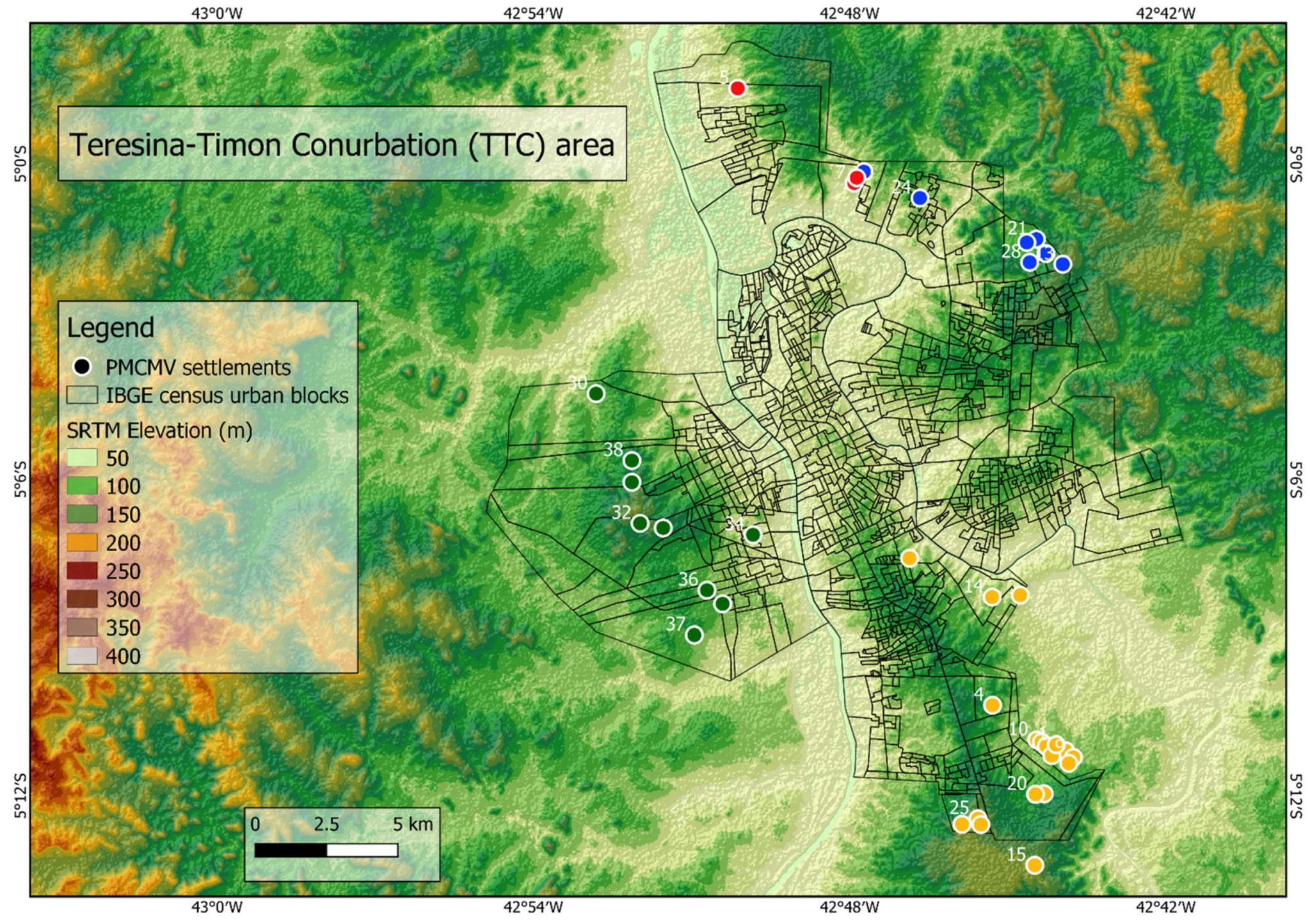
The demographic data were obtained from the IBGE, aggregated at the census block level, and available for 2010 (Figure 2). These data are the most updated data accessible at this spatial scale and the one with the most range of socioeconomic variables. The methodology used to compute the social vulnerability index was described by Freitas et al. [69]. They used a composite vulnerability index constructed from the three synthetic indicators: (i) social structure vulnerability indicator (SSVI), which computes household density and the proportion of literate persons responsible for the households; (ii) household structure vulnerability indicator (HSVI), which computes the proportion of water supply, bathrooms, garbage collection, and electricity in the households; and (iii) urban infrastructure vulnerability indicator (UIV), which computes the proportion of public lighting, paved roads, and arborization in households’ surrounding.
We also used the thirty-eight (38) PMCMV settlements’ locations (Figure 2) to analyze the spatial heat variability. We worked with monthly average air temperature data collected from the Brazilian National Institute of Meteorology (INMET—acronym in Portuguese). We used data from one meteorological station located in the center of the TTC area.
2.3. Spatial Metric for Measuring Urban Sprawl and Its Impacts on the Local Population
From the LULC classifications, we generated synthetic raster data where pixels in the thematic classes Urban area were labeled with value equal ‘1’, and all the other marked with value equal ‘0’. As many indicators that have been developed to evaluate urban sprawl, we here used two metrics proposed by Zhou et al. [34]: land consumption per capita (LCpC) to measure density; and Global Moran’s I coefficient (MCoef) to compute clustering.
Global Moran’s I coefficient is arguably the most commonly used indicator to simultaneously measure spatial autocorrelation based on feature locations and feature values. Inference for Moran’s I is based on a null hypothesis of spatial randomness, and this index tests spatial autocorrelation in geographic features and manipulates three distribution patterns: randomness (I = 0), clustering (I > 1), and dispersion (I < 1) [70]. In our study, the Global Moran’s I coefficient reflects the spatial autocorrelation of the urban land, ranging from −1 to 1. Then, high positive values of MCoef indicate that high-density areas are closely clustered.
Several studies have demonstrated that the MCoef can distinguish compactness from sprawl and is an effective indicator to measure the degree of compactness [34,71,72]. On the other hand, land consumption per capita was calculated as the total urban area by the total population, quantifying each citizen’s developed land. LCpC is a relevant indicator as it can be easily comparable worldwide. We calculated both LCpC and MCoef metrics in two spatial scales: at 30 m × 30 m grid resolution from 2000 to 2018 (Landsat series); and 10 × 10 m grid resolution in 2019 (Sentinel-2).
We also computed the bivariate local Moran’s I to measure the spatial autocorrelation between a range of selected variables, considering the data’s aggregation in a spatial scale at 100 × 100 m grid resolution. We measured the bivariate local Moran’s between: (I) the thematic classes Urban area in 2000, 2010, and 2019 and the land surface temperature (LST) in 2000, 2010, and 2019, respectively; and (B) the social vulnerability index (SVI)—and its synthetic indicators (SSVI, HSVI, and UIV)—in 2010 and the land surface temperature (LST) in 2000, 2010, and 2019.
3. Results
3.1. Patterns of Land Consumption and the Compactness of the TTC Area
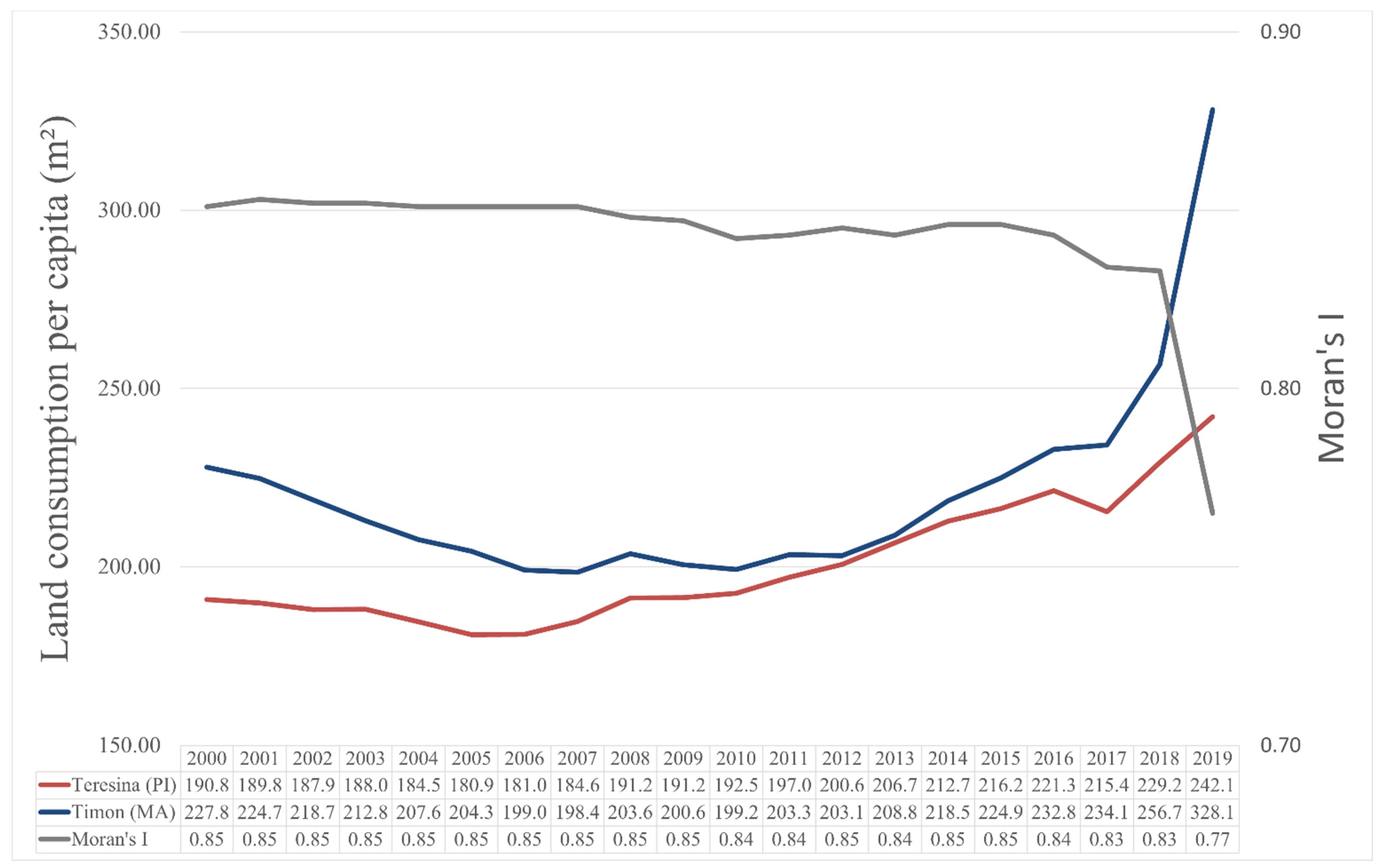
Land consumption per capita in the TTC area had an apparent decreasing trend from 2000 to 2006, followed by a period of increase from 2007 to 2019 (Figure 3). Figure 3 also demonstrates that Teresina and Timon had the same urban sprawl speed [32] and changes in population density. In Teresina, LCpC varied from 190.83 m2 (2000) to 181.00 m2 (2006), and from 184.67 m2 (2007) to 242.11 m2 (2019). In Timon, LCpC varied from 227.89 m2 (2000) to 199.05 m2 (2006), and from 198.42 m2 (2007) to 328.19 m2 (2019).
The results show that Teresina and Timon had similar patterns of LCpC variations. Timon had always remained with LCpC values higher than Teresina over the years. This trend is primarily due to Timon’s low verticalization standards. In this city, the building verticalization is practically nonexistent. In comparison with larger Brazilian urban centers, Teresina also has low building verticalization standards. In Teresina, the verticalization process is still very concentrated in its East zone, where most high-income inhabitants reside [29].
Another possible factor of the LCpC higher values in Timon would be the low land price in this city when compared to Teresina. Part of Timon residents is composed of people who maintain their professional and social routines in Teresina. This trend is explained by the lower land and housing prices in Timon, enabling larger housing units [73]. Like several other examples of dormitory cities in Brazil [74,75], the existing pendulum movement in the urban area of Teresina–Timon helps us to reinforce the hypothesis that the two cities have the same processes and agents of urban expansion. Additionally, it reinforces that these two cities’ urban perimeters form a single unit, despite being under different political-legal arrangements at the municipal and state level.
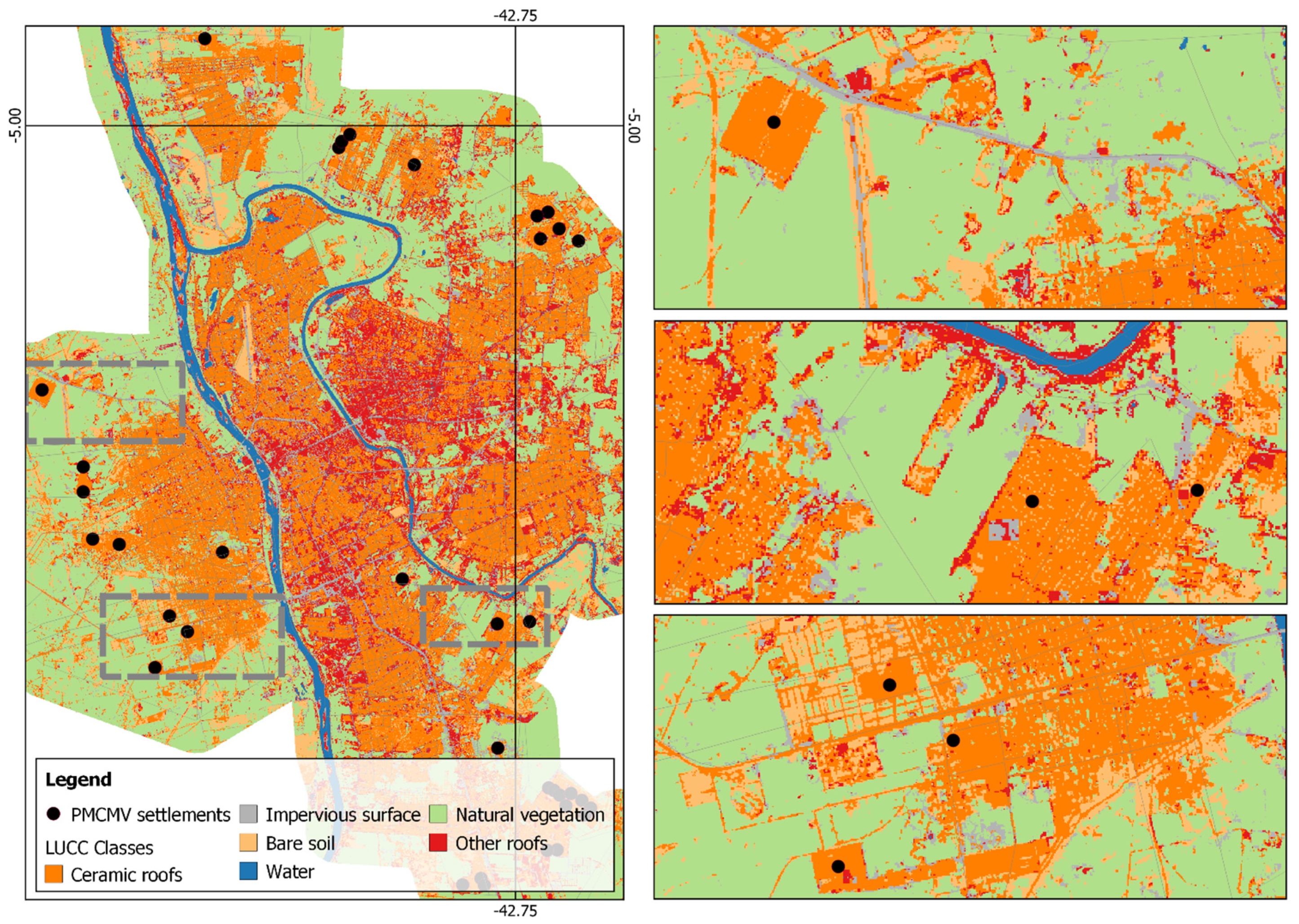
Between 2007 and 2019, Figure 3 shows the LCpC increasing curves for Teresina and Timon. As a result of the urban fabric’s sprawl, we see the emergence of empty urban spaces located among the consolidated central regions of Teresina and Timon and the new areas of peripheral occupation presented in Figure 4 (black dots). There is a real estate speculation of the empty urban spaces and the valorization of areas previously belonging to the rural zones. Besides, such peripheral occupation is always characterized by deficient urban infrastructure that inadequately serves its inhabitants. Our results show that housing estates’ construction is an essential driver of urban expansion in the TTC area.
The MCoef was used to quantify this displacement of the urban fringes to peripheral areas, showing a downward trend (2010–2019) after several years of constant values (2000–2009) (Figure 3). Lower MCoef values mean less compacted and connected urban arrangements. This downward trend is consistent with the existence of empty urban spaces (Figure 4) left by the national housing program’s resumption that favors peripheral areas’ occupation.
3.2. Local Microclimates and the Social Vulnerability
Teresina and Timon are cities with high air temperatures on average. Both cities have been losing part of their vegetation coverage by their urban expansion processes, which is the opposite of an optimum condition for promoting shading, thermal comfort, and maintaining relative air humidity.
When analyzing the average monthly air temperature data, we found an increased trend over 2000 and 2019. In August of 2000, 2010, and 2019 the air temperature measured was 26.87, 27.71, and 28.41 °C, respectively. Climatological studies reported that droughts in the region are becoming more severe, with a significant decreasing trend for annual precipitation, which is associated with the increase in the air temperature [76,77,78].
The land surface temperature (LST) estimates the spatial distribution and variability of the ambient temperature, as a proxy, and it is a critical indicator of the population’s quality of life, as it allows to analyze changes in thermal comfort [46]. In general, the gradual replacement of green areas by residential and commercial ones results in a significant LST increase. Additionally, distinct types of roof material impact temperature dynamics directly. Roof materials are, in general, around 20°C higher than compared with water or vegetation [79].
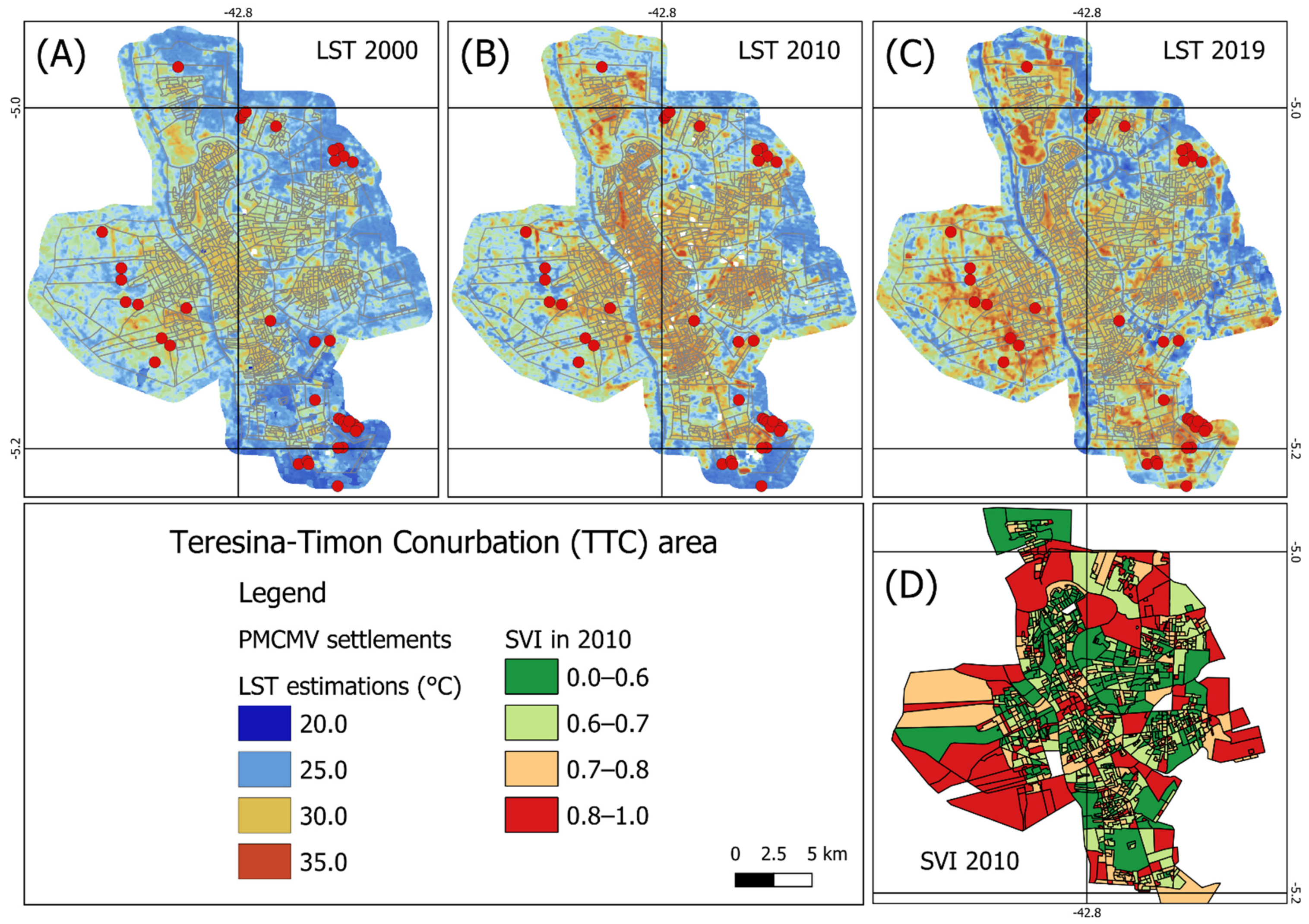
Figure 5 shows the highest temperature values over the urbanized and densely populated areas. Over these years (2000, 2010, and 2019), there is a significant increase in LST in the TTC region. The blue tones (low temperatures) in 2000 were gradually replaced by more red tones (high temperatures) in 2019. In the comparison between the years 2000 and 2019, we demonstrate that there was practically a suppression of the blue areas in the TTC urban fabric. When analyzing each year, it is noticed that, in general, there are peripheral areas with a high-temperature variation, particularly when comparing the 2010 and 2019 maps. There is a high association between the increasing temperature in the areas of the PMCMV settlements.
Figure 5D presents the spatial distribution of the social vulnerability index (SVI) in 2010. Lower values of SVI are showed in the central zones of Teresina–Timon and the East zone of Teresina. Higher values of the SVI are concentrated in the peripherical zones.
Table 3 shows the results of the Bivariate Moran’s I statistic considering: the total urban land in 2000, 2010, and 2019 and the LST in these years, respectively; and the social vulnerability index (SVI)—and its synthetic indicators (SSVI, HSVI, and UIV)—in 2010 and the LST in 2000, 2010, and 2019.
Our results show that the association between land coverage and land surface temperature is significantly positive and increased from 0.538 in 2000, with 0.556 in 2010, and by 0.574 in 2019. Our results confirm that urban impervious surfaces are commonly identified by higher LST when compared to natural LULC types [41]. On the other hand, the association between the SVI and its synthetic indicators is majority negative. However, we see a decrease in these negative trends over the years. This negative association reflects that more vulnerable inhabitants live in areas with low surface temperature values, which would be explained by the natural coverage that remained in peripheral areas.
All the synthetic indicators (SSVI, HSVI, and UIV) maintained this negative association, with the household structure vulnerability indicator (HSVI) having the highest negative values. In 2019, the urban infrastructure vulnerability indicator (UIV) presented a positive association, indicating that even the peripherical zones have become hotter.
Figure 6 shows the variations of LST in the locations where the PMCMV housing complexes were established. These graphics present a clear trend in increasing temperatures after the establishment of such complexes after 2009. We demonstrate that the PMCMV establishment impacted an increase of around 5 to 10 °C in the local microclimate. Even confirming that LST changes are just a proxy for the surface urban heat island (SUHI), our results demonstrate that the housing settlement implementation trend and impacts are evident for thermal comfort quality.
4. Discussion
The TTC area has experienced vast urban sprawl since 1980 [29,32]. The increase of urban developed land is higher than other consolidated metropolitan areas in Brazil [80]. This rapid urban development was directly associated with changes in land consumption per capita. As metrics commonly used to measure the compactness of the urban sprawl, the LCpC and MCoef suggest a less compact urbanizing form with a sprawling trend.
Until 2006, the pace of urban expansion in Teresina and Timon was lower than the pace of population growth, characterizing a process of urban compaction. However, this reality was not shaped by the decrease in the housing deficit. During this period, national housing policies had less expression in the study area, with less area expanding than the population increasing [81,82].
In 2009, the start of the PMCMV housing program resulted in a more intense and peripheral urban occupation. As a rule, Brazilian housing programs moved towards the urban fringe from the acquisition of land farther from the consolidated center and devalued from the real estate point of view, seeking the mass reproduction of housing units at the lowest possible cost. Such practice creates pressure for expanding the urban area, resulting in a higher occupation per capita of the land and a consequent decrease in urban compaction [83,84].
Compared with other international realities, the LCpC values found for the TTC area were similar to those described by Zhou et al. [34] to the megaregion of Beijing, China. However, the MCoef values were much higher for TTC, which shows that this area’s urban expansion process took place in a much more centralized manner, probably due to the lower population pressure. This nature allows an increase in understanding urban expansion characteristics, providing essential public urban planning policies.
Additionally, the two metrics used: LCpC and MCoef, had extreme values in 2019. In this context, higher values of LCpC and lower values of MCoef are directly related to the spatial resolution of the Sentinel-2 satellite, used in the generation of the LULC map for that year. In this work, one of the factors that motivated using different scales of analysis was the growing availability of cloud computing platforms that use remote sensing data from several sensors, such as the Google Earth Engine (GEE). The ease of use of these platforms, added to the wide variety of data, makes it even more important to understand the impacts of methodological choices on urban analysis results. Zhou et al. [34] make evident the advantages of space-time analysis at multiple scales.
In the last two decades, the urban expansion process in the TTC area has impacted social vulnerability in a homogeneous way for the entire region. The dynamics of peripheral land occupations for the implantation of the PMCMV program are the same for Teresina and Timon, resulting in raising the LCpC and decreasing the MCoef. This trend confirms that the urban area has become more widespread, bringing with it all the consequences of this phenomenon, such as distance from the urban center, promotion of urban empty spaces, replacement of green areas by the urban fabric, and environmental impacts.
Recent studies show that planned urban areas are less socially vulnerable than informally developed urban areas. In the context of the TTC area, the PMCMV program is derived from formal urban planning. However, these settlements are usually implemented with less quality of tenure security and housing structure. Then, as demonstrated by Bhanjee and Zhang [49], the implementation of the PMCMV program in the TTC area is more related to sprawled areas with higher social vulnerability, especially considering aspects of quality of life (as thermal comfort) and mobility. Areas with sprawling land use development result in the destruction of the natural environment and agricultural land in the peri-urban areas, generating various forms of pollution, poor sanitation and decreased urban services, and low-density.
Regarding the thermal comfort, the low latitudes of the semiarid areas in Brazil are responsible for the high air temperatures within the cities. Together with LULC changes, they cause changes in energy balance, evidenced by the generation of SUHI [85,86]. SUHI is an important example of anthropogenic impact on the environment, especially in the human–environment interaction through the urbanization process, especially in the context of climate change.
Furthermore, high air temperatures in urban environments are identified as a causal factor in increasing health problems, such as cardiovascular and respiratory diseases. In the TTC area, the average increase in the LST has been associated with the change in LULC and with the PMCMV housing program’ implantation. There was a considered increase in LST, mainly in the areas where the housing complexes were established.
5. Conclusions
Cloud computing platforms are changing the ways we integrate and analyze remote sensing data [32]. Free available data associated with those platforms allow the understanding of the pace of urbanization processes in semiarid environments [87,88]. Historical data linked with population dynamics permits the analysis of interrelationships among urban expansion and the social impacts. Additionally, better spatial resolution data available, like the Sentinel-2 [89], allow the characterization of the urban fabric and its association with the increase of urban artificial impervious surface with the higher patterns of surface urban heat island [90,91].
In this study, we used a combination of spatial data and metrics to discuss the relationships between urban expansion and its impacts on the local population of an urban conurbation in the Brazilian semiarid. We combined remote sensing data and census data to measure land consumption variation over time and the implication of higher urban densities in the local thermal comfort.
Our data and methods used showed to be significantly relevant to the integration of such analyses. Many Latin America studies focus on the urban sprawl or the local temperature increase without integrating these analyses. Monitoring the interlinks among urbanization processes and the social vulnerability is crucial for maintaining sustainable urban centers and allows the settlement of more healthy and inclusive housing environments.
Our main conclusions are: there is a significant gain of using cloud computing platforms and remote sensing data with a higher spatial resolution to compute spatial urban metrics; the PMCMV housing program is one of the main drives of recent urban expansion in the TTC area; and the PMCMV settlements affect the local thermal comfort directly, contributing for intensification in the surface urban heat island.
Our results highlight the importance of quantifying urban sprawl at multiple temporal and spatial scales, considering quantitative indicators. The results described here can improve the understanding of urban social vulnerability and urban planning factors (land use and sprawl) in urban public policies. In the TTC area, as an example of less developed areas in the South globe, such analyses can fill the gaps derived from the lack of field measures.
Author Contributions
E.C. analyzed the data and performed the experiments and computed the data analysis; W.L. and G.E. supervised the conception and design of the analysis and worked on the final manuscript. All authors developed and discussed the manuscript together and finally wrote the paper. All authors have read and agreed to the published version of the manuscript.
Funding
UFPI and IFPI partially funded this research paper.
Institutional Review Board Statement
No appliable.
Informed Consent Statement
No appliable.
Data Availability Statement
No appliable.
Acknowledgments
The authors would like to thank UFPI, IFPI for supporting this research.
Conflicts of Interest
The authors declare no conflict of interest. The funder had no role in the design of the study, in the collection, analysis, or interpretation; in the writing of the manuscript; or in the decision to publish the results.
References
- Seto, K.C.; Fragkias, M.; Güneralp, B.; Reilly, M.K. A Meta-Analysis of Global Urban Land Expansion. PLoS ONE 2011, 6, e23777. [Google Scholar] [CrossRef]
- Shao, Z.; Sumari, N.S.; Portnov, A.; Ujoh, F.; Musakwa, W.; Mandela, P.J. Urban sprawl and its impact on sustainable urban development: A combination of remote sensing and social media data. Geo-Spat. Inf. Sci. 2020, 1–15. [Google Scholar] [CrossRef]
- Prakash, M.; Ramage, S.; Kavvada, A.; Goodman, S. Open Earth Observations for Sustainable Urban Development. Remote Sens. 2020, 12, 1646. [Google Scholar] [CrossRef]
- Chen, G.; Li, X.; Liu, X.; Chen, Y.; Liang, X.; Leng, J.; Xu, X.; Liao, W.; Qiu, Y.; Wu, Q.; et al. Global projections of future urban land expansion under shared socioeconomic pathways. Nat. Commun. 2020, 11, 537. [Google Scholar] [CrossRef] [Green Version]
- Dobbs, C.; Escobedo, F.J.; Clerici, N.; De La Barrera, F.; Eleuterio, A.A.; MacGregor-Fors, I.; Reyes-Paecke, S.; Vásquez, A.; Camaño, J.D.Z.; Hernández, H.J. Urban ecosystem Services in Latin America: Mismatch between global concepts and regional realities? Urban Ecosyst. 2019, 22, 173–187. [Google Scholar] [CrossRef]
- Gaviria, S.; Goldwyn, E.; Liu, Y.; Galarza, N.; Angel, S. Invisible walls: Measuring the impact of organized violence on urban expansion. Cities 2020, 97, 102498. [Google Scholar] [CrossRef]
- Ewing, R.; Hamidi, S. Compactness versus Sprawl: A review of recent evidence from the United States. J. Plan. Lit. 2015, 30, 413–432. [Google Scholar] [CrossRef]
- Bongaarts, J.; O’Neill, B.C. Global warming policy: Is population left out in the cold? Science 2018, 361, 650–652. [Google Scholar] [CrossRef]
- Salim, Z.; Bosco, F.J. Latin American Cities. Placing Latin America: Contemporary Themes in Geography; Rowman & Littlefield Publishers: London, UK, 2020; p. 61. [Google Scholar]
- Rovai, M.; Zetti, I.; Lucchesi, F.; Rossi, M.; Andreoli, M. Peri-urban open spaces and sustainable urban development between value and consumption. In Values and Functions for Future Cities; Springer: Berlin/Heidelberg, Germany, 2020; pp. 249–265. [Google Scholar]
- United Nations. World Urbanization Prospects: The 2014 Revision, Highlights; ONU: New York, NY, USA, 2014; Volume 1. [Google Scholar]
- Acuto, M.; Parnell, S.; Seto, K.C. Building a global urban science. Nat. Sustain. 2018, 1, 2–4. [Google Scholar] [CrossRef]
- Rivera, M. Political criteria for Sustainable Development Goal (SDG) selection and the role of the urban dimension. Sustainability 2013, 5, 5034–5051. [Google Scholar] [CrossRef] [Green Version]
- Bilal, U.; Alazraqui, M.; Caiaffa, W.T.; Lopez-Olmedo, N.; Martinez-Folgar, K.; Miranda, J.J.; Rodriguez, D.A.; Vives, A.; Diez-Roux, A.V. Inequalities in life expectancy in six large Latin American cities from the SALURBAL study: An ecological analysis. Lancet Planet. Health 2019, 3, e503–e510. [Google Scholar] [CrossRef] [Green Version]
- Rausky, M.E.; Chaves, M. Living and Working in Poverty in Latin America; Springer: Berlin/Heidelberg, Germany, 2019. [Google Scholar]
- Molina, I.; Czischke, D.; Rolnik, R. Housing policy issues in contemporary South America: An introduction. Int. J. Hous. Policy 2019, 19, 277–287. [Google Scholar] [CrossRef] [Green Version]
- Roberts, B.R.; Wilson, R.H. Urban Segregation and Governance in the Americas; Springer: Berlin/Heidelberg, Germany, 2009. [Google Scholar]
- Rotondano, R.O. Brazilian apartheid: Racism and segregation in Salvador, Brazil. Int. J. Sociol. Soc. Policy 2019, 39, 950–961. [Google Scholar] [CrossRef]
- Creţan, R.; Málovics, G.; Méreiné-Berki, B. On the perpetuation and contestation of racial stigma: Urban Roma in a disadvantaged neighbourhood of Szeged. Geogr. Pannonica 2020, 24, 294–310. [Google Scholar] [CrossRef]
- Inostroza, L.; Baur, R.; Csaplovics, E. Urban sprawl and fragmentation in Latin America: A dynamic quantification and characterization of spatial patterns. J. Environ. Manag. 2013, 115, 87–97. [Google Scholar] [CrossRef] [PubMed]
- Leite, C.; Acosta, C.; Militelli, F.; Jajamovich, G.; Wilderom, M.; Bonduki, N.; Somekh, N.; Herling, T. Social urbanism in Latin America. In Social Urbanism in Latin America; Springer: Berlin/Heidelberg, Germany, 2020; pp. 3–21. [Google Scholar]
- Ojima, R.; Hogan, D.J. Mobility, Urban sprawl and environmental risks in brazilian urban agglomerations:challenges for urban sustainability. In Urban Population-Environment Dynamics in the Developing World: Case Studies and Lessons Learned; De Sherbiniin, A., Rahman, A., Barbieri, A., Fotso, J.C., Zhu, Y., Eds.; Committee for International Cooperation in National Research in Demography: Paris, France, 2009; pp. 281–316. ISBN 2-910053-35-0. [Google Scholar]
- Sabatini, F. The Social Spatial Segregation in the Cities of Latin America; Inter-American Development Bank: Washington, DC, USA, 2003. [Google Scholar]
- Sperandelli, D.I.; Dupas, F.A.; Pons, N.A.D. Dynamics of Urban Sprawl, Vacant Land, and Green Spaces on the Metropolitan Fringe of São Paulo, Brazil. J. Urban Plan. Dev. 2013, 139, 274–279. [Google Scholar] [CrossRef]
- Klink, J.; Denaldi, R. On financialization and state spatial fixes in Brazil. A geographical and historical interpretation of the housing program My House My Life. Habitat Int. 2014, 44, 220–226. [Google Scholar] [CrossRef]
- Mourougane, A.; Pisu, M. Promoting Infrastructure Development in Brazil. 2011. Available online: https://ideas.repec.org/p/oec/ecoaaa/898-en.html (accessed on 17 April 2021).
- Shimbo, L. An unprecedented alignment: State, finance, construction and housing production in Brazil since the 2000s. Int. J. Hous. Policy 2019, 19, 337–353. [Google Scholar] [CrossRef]
- Filho, W.L.F.C.; Santiago, D.D.B.; De Oliveira-Júnior, J.F.; Junior, C.A.D.S. Impact of urban decadal advance on land use and land cover and surface temperature in the city of Maceió, Brazil. Land Use Policy 2019, 87, 104026. [Google Scholar] [CrossRef]
- De Espindola, G.M.; Carneiro, E.L.N.D.C.; Façanha, A.C. Four decades of urban sprawl and population growth in Teresina, Brazil. Appl. Geogr. 2017, 79, 73–83. [Google Scholar] [CrossRef]
- Qian, Y.; Zhou, W.; Yan, J.; Li, W.; Han, L. Comparing machine learning classifiers for object-based land cover classification using very high resolution imagery. Remote Sens. 2015, 7, 153–168. [Google Scholar] [CrossRef]
- Wu, W.; Zhao, S.; Zhu, C.; Jiang, J. A comparative study of urban expansion in Beijing, Tianjin and Shijiazhuang over the past three decades. Landsc. Urban Plan. 2015, 134, 93–106. [Google Scholar] [CrossRef]
- Carneiro, E.; Lopes, W.; Espindola, G. Urban Land Mapping Based on Remote Sensing Time Series in the Google Earth Engine Platform: A Case Study of the Teresina-Timon Conurbation Area in Brazil. Remote Sens. 2021, 13, 1338. [Google Scholar] [CrossRef]
- Hamidi, S.; Ewing, R. A longitudinal study of changes in urban sprawl between 2000 and 2010 in the United States. Landsc. Urban Plan. 2014, 128, 72–82. [Google Scholar] [CrossRef]
- Zhou, W.; Jiao, M.; Yu, W.; Wang, J. Urban sprawl in a megaregion: A multiple spatial and temporal perspective. Ecol. Indic. 2019, 96, 54–66. [Google Scholar] [CrossRef]
- Li, X.; Gong, P.; Liang, L. A 30-year (1984–2013) record of annual urban dynamics of Beijing City derived from Landsat data. Remote Sens. Environ. 2015, 166, 78–90. [Google Scholar] [CrossRef]
- Lu, Y.; Coops, N.C.; Hermosilla, T. Estimating urban vegetation fraction across 25 cities in pan-Pacific using Landsat time series data. ISPRS J. Photogramm. Remote Sens. 2017, 126, 11–23. [Google Scholar] [CrossRef]
- Song, X.-P.; Sexton, J.O.; Huang, C.; Channan, S.; Townshend, J.R. Characterizing the magnitude, timing and duration of urban growth from time series of Landsat-based estimates of impervious cover. Remote Sens. Environ. 2016, 175, 1–13. [Google Scholar] [CrossRef]
- Iannelli, G.C.; Gamba, P. Jointly exploiting Sentinel-1 and Sentinel-2 for urban mapping. In Proceedings of the IGARSS 2018-2018IEEE International Geoscience and Remote Sensing Symposium, Valencia, Spain, 22–27 July 2018; pp. 8209–8212. [Google Scholar]
- El Mendili, L.; Puissant, A.; Chougrad, M.; Sebari, I. Towards a Multi-Temporal Deep Learning Approach for Mapping Urban Fabric Using Sentinel 2 Images. Remote Sens. 2020, 12, 423. [Google Scholar] [CrossRef] [Green Version]
- Pesaresi, M.; Corbane, C.; Julea, A.; Florczyk, A.J.; Syrris, V.; Soille, P. Assessment of the Added-Value of Sentinel-2 for Detecting Built-up Areas. Remote Sens. 2016, 8, 299. [Google Scholar] [CrossRef] [Green Version]
- Goldblatt, R.; Addas, A.; Crull, D.; Maghrabi, A.; Levin, G.; Rubinyi, S. Remotely Sensed Derived Land Surface Temperature (LST) as a Proxy for Air Temperature and Thermal Comfort at a Small Geographical Scale. Land 2021, 10, 410. [Google Scholar] [CrossRef]
- Chen, M.; Zhou, Y.; Hu, M.; Zhou, Y. Influence of Urban Scale and Urban Expansion on the Urban Heat Island Effect in Metropolitan Areas: Case Study of Beijing–Tianjin–Hebei Urban Agglomeration. Remote Sens. 2020, 12, 3491. [Google Scholar] [CrossRef]
- Peng, S.; Piao, S.; Ciais, P.; Friedlingstein, P.; Ottle, C.; Bréon, F.-M.; Nan, H.; Zhou, L.; Myneni, R.B. Surface Urban Heat Island Across 419 Global Big Cities. Environ. Sci. Technol. 2011, 46, 696–703. [Google Scholar] [CrossRef]
- Srivastava, P.; Majumdar, T.; Bhattacharya, A.K. Surface temperature estimation in Singhbhum Shear Zone of India using Landsat-7 ETM+ thermal infrared data. Adv. Space Res. 2009, 43, 1563–1574. [Google Scholar] [CrossRef]
- Liu, S.; Long, B.; Pan, Z.; Lun, F.; Song, Y.; Yuan, W.; Huang, N.; Zhang, Z.; Ma, S. Evaluation of Climatic Comfort of Living Environment based on Age Differentials in Beijing-Tianjin-Hebei Area. Ecosyst. Health Sustain. 2020, 6, 1843371. [Google Scholar] [CrossRef]
- Wang, Y.; Xu, M.; Li, J.; Jiang, N.; Wang, D.; Yao, L.; Xu, Y. The Gradient Effect on the Relationship between the Underlying Factor and Land Surface Temperature in Large Urbanized Region. Land 2020, 10, 20. [Google Scholar] [CrossRef]
- Liu, Y.; Li, H.; Gao, P.; Zhong, C. Monitoring the Detailed Dynamics of Regional Thermal Environment in a Developing Urban Agglomeration. Sensors 2020, 20, 1197. [Google Scholar] [CrossRef] [Green Version]
- Sabrin, S.; Karimi, M.; Fahad, G.R.; Nazari, R. Quantifying environmental and social vulnerability: Role of urban Heat Island and air quality, a case study of Camden, NJ. Urban Clim. 2020, 34, 100699. [Google Scholar] [CrossRef]
- Bhanjee, S.; Zhang, S. Do urban planning and sprawl affect social vulnerability? An assessment of Dar es Salaam. Dev. S. Afr. 2021, 38, 189–207. [Google Scholar] [CrossRef]
- Mereine Berki, B.; Málovics, G.; Toth, J.; Creţan, R. The Role of Social Capital and Interpersonal Relations in The Alleviation of Extreme Poverty And Spatial Segregation Of Romani People In Szeged. J. Urban Reg. Anal. 2017, 9, 33–50. [Google Scholar]
- Málovics, G.; Creţan, R.; Méreiné Berki, B.; Tóth, J. Urban Roma, segregation and place attachment in Szeged, Hungary. Area 2019, 51, 72–83. [Google Scholar] [CrossRef]
- Khan, S. Vulnerability assessments and their planning implications: A case study of the Hutt Valley, New Zealand. Nat. Hazards 2012, 64, 1587–1607. [Google Scholar] [CrossRef]
- Spielman, S.E.; Tuccillo, J.; Folch, D.C.; Schweikert, A.; Davies, R.; Wood, N.; Tate, E. Evaluating social vulnerability indicators: Criteria and their application to the Social Vulnerability Index. Nat. Hazards 2020, 100, 417–436. [Google Scholar] [CrossRef] [Green Version]
- Connolly, J.J. From Systems Thinking to Systemic Action: Social Vulnerability and the Institutional Challenge of Urban Resilience. City Community 2018, 17, 8–11. [Google Scholar] [CrossRef]
- Freitas, C.R.; D’Avignon, A.L.D.A.; Castro, A.C. Urban social vulnerability and climate change in Rio de Janeiro city associated with population mobility. J. Environ. Policy Plan. 2019, 21, 797–810. [Google Scholar] [CrossRef]
- Hummell, B.M.D.L.; Cutter, S.L.; Emrich, C.T. Social Vulnerability to Natural Hazards in Brazil. Int. J. Disaster Risk Sci. 2016, 7, 111–122. [Google Scholar] [CrossRef] [Green Version]
- Tascón-González, L.; Ferrer-Julià, M.; Ruiz, M.; García-Meléndez, E. Social Vulnerability Assessment for Flood Risk Analysis. Water 2020, 12, 558. [Google Scholar] [CrossRef] [Green Version]
- Aroca-Jimenez, E.; Bodoque, J.M.; Garcia, J.A.; Diez-Herrero, A. Construction of an integrated social vulnerability index in urban areas prone to flash flooding. Nat. Hazards Earth Syst. Sci. 2017, 17, 1541–1557. [Google Scholar] [CrossRef] [Green Version]
- Gu, H.; Du, S.; Liao, B.; Wen, J.; Wang, C.; Chen, R.; Chen, B. A hierarchical pattern of urban social vulnerability in Shanghai, China and its implications for risk management. Sustain. Cities Soc. 2018, 41, 170–179. [Google Scholar] [CrossRef]
- Fahy, B.; Brenneman, E.; Chang, H.; Shandas, V. Spatial analysis of urban flooding and extreme heat hazard potential in Portland, OR. Int. J. Disaster Risk Reduct. 2019, 39, 101117. [Google Scholar] [CrossRef]
- Hossain, M.K.; Meng, Q. A thematic mapping method to assess and analyze potential urban hazards and risks caused by flooding.Comput. Environ. Urban Syst. 2020, 79, 101417. [Google Scholar] [CrossRef]
- IBGE. Censo Demográfico 2010. In Síntese de Indicadores: Rio de Janeiro. 2013. Available online: https://biblioteca.ibge.gov.br/visualizacao/periodicos/93/cd_2010_caracteristicas_populacao_domicilios.pdf (accessed on 17 April 2021).
- Marengo, J.A.; Cunha, A.P.; Soares, W.R.; Torres, R.R.; Alves, L.M.; de Barros Brito, S.S.; Cuartas, L.A.; Leal, K.; Ribeiro Neto, G.; Alvalá, R.C.S.; et al. Increase Risk of Drought in the Semiarid Lands of Northeast Brazil Due to Regional Warming above 4 °C. In Climate Change Risks in Brazil; Springer International Publishing: Cham, Switzerland, 2019; pp. 181–200. [Google Scholar]
- Paredes-Trejo, F.J.; Barbosa, H.; Kumar, T.L. Validating CHIRPS-based satellite precipitation estimates in Northeast Brazil. J. Arid. Environ. 2017, 139, 26–40. [Google Scholar] [CrossRef]
- Dos Santos, S.M.; de Farias, M.M.M. Potential for rainwater harvesting in a dry climate: Assessments in a semiarid region in northeast Brazil. J. Clean. Prod. 2017, 164, 1007–1015. [Google Scholar] [CrossRef]
- Lemos, M.C.; Finan, T.J.; Fox, R.W.; Nelson, D.R.; Tucker, J. The Use of Seasonal Climate Forecasting in Policymaking: Lessons from Northeast Brazil. Clim. Chang. 2002, 55, 479–507. [Google Scholar] [CrossRef]
- Alencar, A.; Shimbo, J.Z.; Lenti, F.; Marques, C.B.; Zimbres, B.; Rosa, M.; Arruda, V.; Castro, I.; Ribeiro, J.F.M.; Varela, V.; et al. Mapping Three Decades of Changes in the Brazilian Savanna Native Vegetation Using Landsat Data Processed in the Google Earth Engine Platform. Remote Sens. 2020, 12, 924. [Google Scholar] [CrossRef] [Green Version]
- Ermida, S.L.; Soares, P.; Mantas, V.; Göttsche, F.-M.; Trigo, I.F. Google earth engine open-source code for land surface tem-perature estimation from the landsat series. Remote Sens. 2020, 12, 1471. [Google Scholar] [CrossRef]
- De Freitas Rocha, A.T.; Mira de Espindola, G.; Araujo Soares, M.R.; de Ribamar de Sousa Rocha, J.; Nery Costa, C.H. Visceralleishmaniasis and vulnerability conditions in an endemic urban area of Northeastern Brazil. Trans. R. Soc. Trop. Med. Hyg. 2018, 112, 317–325. [Google Scholar] [CrossRef] [PubMed]
- Estiri, H. Tracking urban sprawl: Applying Moran’s I technique in developing sprawl detection models. Emergent Placemaking 2012, 47–53. [Google Scholar]
- Rahman, M.S. Quantifying urban form-compactness versus sprawl: An analysis of Chittagong and Sylhet metropolitan cities. Jahangirnagar University. Plan. Rev. 2012, 10, 39–50. [Google Scholar]
- Tsai, Y.-H. Quantifying Urban Form: Compactness versus ‘Sprawl’. Urban Stud. 2005, 42, 141–161. [Google Scholar] [CrossRef]
- de Magalhães, D.J.A.V. Localização residencial e acessibilidade ao local de trabalho dentro do aglomerado urbano formado pelos municípios de Teresina (PI) e Timon (MA). Anais 2016, 34, 1–20. [Google Scholar]
- Ojima, R.; Marandola, E., Jr.; Pereira, R.H.M.; da Silva, R.B. O estigma de morar longe da cidade: Repensando o consenso sobre as” cidades-dormitório” no Brasil. Cad. Metrópole 2010, 12, 395–415. [Google Scholar]
- Ojima, R.; Pereira, R.H.M.; da Silva, R.B. Cidades-dormitório e a mobilidade pendular: Espaços da desigualdade na redis-tribuição dos riscos socioambientais? Anais 2016, 36, 1–20. [Google Scholar]
- Marengo, J.A.; Bernasconi, M. Regional differences in aridity/drought conditions over Northeast Brazil: Present state and future projections. Clim. Chang. 2015, 129, 103–115. [Google Scholar] [CrossRef]
- Marengo, J.A.; Torres, R.R.; Alves, L.M. Drought in Northeast Brazil—Past, present, and future. Theor. Appl. Clim. 2017, 129, 1189–1200. [Google Scholar] [CrossRef]
- Marengo, J.A.; Cunha, A.P.M.A.; Nobre, C.A.; Neto, G.G.R.; Magalhaes, A.R.; Torres, R.R.; Sampaio, G.; Alexandre, F.; Alves, L.M.; Cuartas, L.A.; et al. Assessing drought in the drylands of northeast Brazil under regional warming exceeding 4 °C. Nat. Hazards 2020, 103, 2589–2611. [Google Scholar] [CrossRef]
- Leuzinger, S.; Vogt, R.; Körner, C. Tree surface temperature in an urban environment. Agric. For. Meteorol. 2010, 150, 56–62. [Google Scholar] [CrossRef]
- Moschetto, F.; Ribeiro, R.; De Freitas, D. Urban expansion, regeneration and socioenvironmental vulnerability in a mangrove ecosystem at the southeast coastal of São Paulo, Brazil. Ocean Coast. Manag. 2020, 200, 105418. [Google Scholar] [CrossRef]
- Valença, M.M.; Bonates, M.F. The trajectory of social housing policy in Brazil: From the National Housing Bank to the Ministry of the Cities. Habitat Int. 2010, 34, 165–173. [Google Scholar] [CrossRef] [Green Version]
- Ren, X. Governing the Informal: Housing Policies Over Informal Settlements in China, India, and Brazil. Hous. Policy Debate 2018, 28, 79–93. [Google Scholar] [CrossRef]
- Biderman, C.; Hiromoto, M.H.; Ramos, F.R. Brazilian Housing Program Minha Casa Minha Vida: Effect on Urban Sprawl; Lincoln Institute of Land Policy: Cambridge, MA, USA, 2018. [Google Scholar]
- Neto, P.N.; Moreira, T.A.; Schussel, Z.D.G.L. Housing Policy. A Critical Analysis on the Brazilian Experience. TeMA-J. Land Use Mobil. Environ. 2012, 5, 65–76. [Google Scholar]
- Mohammad, P.; Goswami, A.; Bonafoni, S. The Impact of the Land Cover Dynamics on Surface Urban Heat Island Variations in Semi-Arid Cities: A Case Study in Ahmedabad City, India, Using Multi-Sensor/Source Data. Sensors 2019, 19, 3701. [Google Scholar] [CrossRef] [Green Version]
- Haashemi, S.; Weng, Q.; Darvishi, A.; Alavipanah, S.K. Seasonal Variations of the Surface Urban Heat Island in a Semi-Arid City. Remote Sens. 2016, 8, 352. [Google Scholar] [CrossRef] [Green Version]
- Tamiminia, H.; Salehi, B.; Mahdianpari, M.; Quackenbush, L.; Adeli, S.; Brisco, B. Google Earth Engine for geo-big data ap-plications: A meta-analysis and systematic review. ISPRS J. Photogramm. Remote Sens. 2020, 164, 152–170. [Google Scholar] [CrossRef]
- Mugiraneza, T.; Nascetti, A.; Ban, Y. Continuous Monitoring of Urban Land Cover Change Trajectories with Landsat Time Series and LandTrendr-Google Earth Engine Cloud Computing. Remote Sens. 2020, 12, 2883. [Google Scholar] [CrossRef]
- Mohammadnejad, V. Urban lands Extraction from Sentinel 1 and 2 satellite imagery based on Google Earth Engine (GEE). Geogr. Urban Plan. Res. GUPR 2020, 8, 613–630. [Google Scholar]
- Ranagalage, M.; Ratnayake, S.S.; Dissanayake, D.; Kumar, L.; Wickremasinghe, H.; Vidanagama, J.; Cho, H.; Udagedara, S.; Jha, K.K.; Simwanda, M.; et al. Spatiotemporal Variation of Urban Heat Islands for Implementing Nature-Based Solutions: A Case Study of Kurunegala, Sri Lanka. ISPRS Int. J. Geo-Inf. 2020, 9, 461. [Google Scholar] [CrossRef]
- Wang, Z.; Liu, M.; Liu, X.; Meng, Y.; Zhu, L.; Rong, Y. Spatio-Temporal evolution of surface urban heat islands in the Chang-Zhu-Tan urban agglomeration. Phys. Chem. Earth Parts A/B/C 2020, 117, 102865. [Google Scholar] [CrossRef]
Figure 1.
Location of the study area: (A) Brazil in South America; (B) Maranhão (MA) and Piauí (PI) Brazilian states; (C) Timon—MA and Teresina—PI urban areas in the MultiSpectral Instrument (MSI) Sentinel-2A color composition, bands 4(R)3(G)2(B), acquisition date in 8 November 2019. In red, annual urban sprawl from 1985 to 2018.

Figure 2.
2010 urban census block boundaries in the TTC area (black geometry). Location of the federal housing program ‘My House My Life’ settlements constructed after 2009 (red dots). Shuttle Radar Topography Mission (SRTM) elevation map (background).
Figure 2.
2010 urban census block boundaries in the TTC area (black geometry). Location of the federal housing program ‘My House My Life’ settlements constructed after 2009 (red dots). Shuttle Radar Topography Mission (SRTM) elevation map (background).

Figure 3.
Land consumption per capita (LCpC) and the Global Moran’s I coefficient (MCoef) of urban lands in the TTC area from 2000 to 2019.
Figure 3.
Land consumption per capita (LCpC) and the Global Moran’s I coefficient (MCoef) of urban lands in the TTC area from 2000 to 2019.

Figure 4.
2019 LULC map derived from Sentinel-2 data. Displacement of the PMCMV settlements within the urban fabric (on the right).
Figure 4.
2019 LULC map derived from Sentinel-2 data. Displacement of the PMCMV settlements within the urban fabric (on the right).

Figure 5.
Land surface temperature (LST) estimations in the Teresina–Timon conurbation area in 2000 (A), 2010 (B), and 2019 (C). Spatial distribution of the social vulnerability index (SVI) in 2010 (D).
Figure 5.
Land surface temperature (LST) estimations in the Teresina–Timon conurbation area in 2000 (A), 2010 (B), and 2019 (C). Spatial distribution of the social vulnerability index (SVI) in 2010 (D).

Figure 6.
Land surface temperature (LST) in 2000, 2010, and 2019 for each location where a PMCMV settlement was established, grouped into the directions: North, East, West, and South in the TTC area.
Figure 6.
Land surface temperature (LST) in 2000, 2010, and 2019 for each location where a PMCMV settlement was established, grouped into the directions: North, East, West, and South in the TTC area.


Table 1.
Socioeconomic characterization of the Teresina–Timon conurbation area.
| Characteristics | Teresina | Timon |
|---|---|---|
| Brazilian state | Piauí (PI) | Maranhão (MA) |
| Population estimated in 2019 | 864,845 inhabitants | 169,107 inhabitants |
| Population surveyed in 2010 | 814,230 inhabitants | 155,460 inhabitants |
| Urban population in 2010 | 80.54% | 71.15% |
| Population density in 2010 | 584.94 inhabitants/km2 | 89.18 inhabitants/km2 |
| Total estimated urban area in 2019 | 168.64 km2 | 39.49 km2 |
| Human Development Index (HDI) in 2010 | 0.751 | 0.649 |
| Gross Domestic Product (GDP) per capita | USD 6785.28 | USD 3245.85 |
Table 2.
Temporal coverage considered for Landsat and Sentinel-2 data.
| Sensor/Satellite 1 | Filtered Collection | Spatial Resolution |
|---|---|---|
| TM Landsat-5 (L5) | 2000 to 2011 | 30 m |
| ETM+ Landsat-7 (L7) | 2012 | 30 m |
| OLI Landsat-8 (L8) | 2013 to 2018 2019 (TIR only) | 30 m |
| MSI Sentinel-2 (S2) | 2019 | 10 m |
| MSI Sentinel-2 (S2) | 2019 | 20 m (Band 11 only) |
1 Thematic Mapper (TM) Landsat-5 (L5), Enhanced Thematic Mapper Plus (ETM+) Landsat-7 (L7), Operational Land Imager (OLI) Landsat-8 (L8), and MultiSpectral Instrument (MSI) Sentinel-2 (S2).
Table 3.
Bivariate Moran’s I computed between: the thematic classes Urban area and the land surface temperature; and the social vulnerability index (SVI)—and its synthetic indicators (SSVI, HSVI, and UIV)—in 2010 and the land surface temperature.
Table 3.
Bivariate Moran’s I computed between: the thematic classes Urban area and the land surface temperature; and the social vulnerability index (SVI)—and its synthetic indicators (SSVI, HSVI, and UIV)—in 2010 and the land surface temperature.
| Bivariate Moran’s I | LST 1 2000 | LST 2010 | LST 2019 |
|---|---|---|---|
| Urban 2000 | 0.538 | - | - |
| Urban 2010 | - | 0.556 | - |
| Urban 2019 | - | - | 0.574 |
| SVI 1 | −0.119 | −0.098 | −0.063 |
| SSVI | −0.114 | −0.075 | −0.074 |
| HSVI | −0.133 | −0.084 | −0.015 |
| UIV | −0.123 | −0.103 | 0.096 |
1 Land surface temperature (LST). Social vulnerability index (SVI). Social structure vulnerability indicator (SSVI). Household structure vulnerability indicator (HSVI). Urban infrastructure vulnerability indicator (UIV).
Publisher’s Note: MDPI stays neutral with regard to jurisdictional claims in published maps and institutional affiliations. |
© 2021 by the authors. Licensee MDPI, Basel, Switzerland. This article is an open access article distributed under the terms and conditions of the Creative Commons Attribution (CC BY) license (https://creativecommons.org/licenses/by/4.0/).
Share and Cite
MDPI and ACS Style
Carneiro, E.; Lopes, W.; Espindola, G. Linking Urban Sprawl and Surface Urban Heat Island in the Teresina–Timon Conurbation Area in Brazil. Land 2021, 10, 516. https://0-doi-org.brum.beds.ac.uk/10.3390/land10050516
AMA Style
Carneiro E, Lopes W, Espindola G. Linking Urban Sprawl and Surface Urban Heat Island in the Teresina–Timon Conurbation Area in Brazil. Land. 2021; 10(5):516. https://0-doi-org.brum.beds.ac.uk/10.3390/land10050516
Chicago/Turabian StyleCarneiro, Eduilson, Wilza Lopes, and Giovana Espindola. 2021. "Linking Urban Sprawl and Surface Urban Heat Island in the Teresina–Timon Conurbation Area in Brazil" Land 10, no. 5: 516. https://0-doi-org.brum.beds.ac.uk/10.3390/land10050516
Note that from the first issue of 2016, this journal uses article numbers instead of page numbers. See further details here.