Landslide Hazard Assessment in a Monoclinal Setting (Central Italy): Numerical vs. Geomorphological Approach

Abstract

A correct landslide hazard assessment (LHA) is fundamental for any purpose of territorial planning. In Italy, the methods currently in use to achieve this objective alternate between those based on mainly qualitative (geomorphological) and quantitative (statistical–numerical) approaches. The present study contributes to the evaluation of the best procedure to be implemented for LHA, comparing the results obtained using two different approaches (geomorphological and numerical) in a territorial context characterized by conditioning and triggering factors, favorable to the instability of the slopes. The results obtained, although preliminary, evidence the respective limitations of the methods and demonstrate how a combined approach can certainly provide mutual advantages, by addressing the choice of the best numerical model through direct observations and surveys.

1. Introduction

Landslide hazard assessment (LHA) is a challenging task for the prevention and prediction of a territory for local land management and security services. Proper management of landslide hazard, as well as saving human lives, can minimize socioeconomical impact that in many developing countries may equal a large percentage of the gross national product [1,2]. LHA is usually based on the spatial and temporal probability of landslide occurrences and is performed following three main steps: (i) the creation of a phenomenon inventory, (ii) a landslide susceptibility analysis and (iii) a landslide hazard analysis [3,4,5].

In Italy, the National Plan for Hydrogeological Risk Assessment (PAI) [6] is the cognitive, regulatory and technical–operational tool through which actions, interventions and rules concerning the defense against hydrogeological risk of the territory are planned and scheduled. Although the term LHA (in its Italian translation) is often mentioned within the PAI, the significance is at times contradictory, and the products of the Plan (maps, inventory sheets, analyses, etc.) rarely come from the steps described above; on the contrary, they are often realized based on an empirical approach and basic available data. In particular, hazard, vulnerability and risk degree (the latter in terms of exposed value) is closely linked to the quality of the expertise, while only in a few cases have specific studies (numerical models, statistical/probabilistic approaches) been applied [7,8,9,10,11]. As a consequence, the representation of the landslide hazard that emerges in some areas of the Italian territory can be over/underestimated, and divergent opinions may arise among technicians and public administrators. This problem, among other aspects, has also been highlighted in other countries of the European Union such as France [3,4,12,13].

In a more general context, the methods currently in use in Italy for LHA include two main types of approach: the field-based qualitative approach and the data-driven quantitative one [14]. The former type includes the so-called ”geomorphological” methods [3,5,6,7,8,15,16,17], while the latter includes the statistical analyses (i.e., bivariate and multivariate statistical techniques, [7,18,19,20,21,22]) and the deterministic methods that involve, among others, the analysis of specific sites or slopes based on numerical models [23,24,25,26,27,28,29,30].

The present work compares the results of a landslide analysis carried out in a sample area using both geomorphological and numerical approaches. The area chosen for the analysis is located in a high hilly sector of the Adriatic side of the Central Apennines (Italy), characterized by the presence of monoclinal reliefs and typical cuesta morphologies, formed by differential tectonic movements in a recent uplift area [31,32]. Despite the relative simplicity of the geological model, these contexts can generate complex mass movements, both for characteristics (type of movement) and size (extension and depth of the failure zone) and kinematics (velocity and return time) and consequently represent high hazard conditions in the presence of built-up areas and/or infrastructures. The LHA (following the significance given by Italian PAI) is typically conducted based on a geomorphological approach and an expert judgment as regards the attribution of the degree of vulnerability and the exposed value. For any reclassification of the degree of risk, site-specific analyses (i.e., instrumental monitoring, geognostic bore-holes, geophysical prospecting) or the use of numerical models (slope stability analyses) are usually required by Italian guidelines. Nevertheless, both types of investigations proposed have limitations. In the first case, the non-negligible costs of direct surveys and prospecting limit the representativeness of the surveys themselves; in the case of numerical models, on the other hand, reliability is mainly linked to a correct choice of input parameters, is sometimes not homogeneous in the area considered and is often deduced from bibliographic data.

In this study, using finite-difference software (ITASCA FLAC/Slope v.8.0 [33]) the factor of safety (FoS) was calculated on representative slope sections where detailed geomorphological surveys highlighted the presence of gravitational phenomena or stability conditions. This analysis, in particular, refers to medium-to-low depth landslides, while more complex phenomena (as specified in the following paragraphs) recognized in the area and associated with deep-seated gravitational slope deformations were not included in the study [34,35].

The objective of this study was to clarify the role, usefulness and limits of the different methods to be used in the LHA and also provide useful information for their correct use in any context of territorial planning where specific indications have not been provided. A further aim was to demonstrate a combined and intelligent use of the two methods, pending clearer and universally accepted regulatory indications on the methods to be used for the LHA, which seems at the moment the most suitable choice both in economic and safety terms.

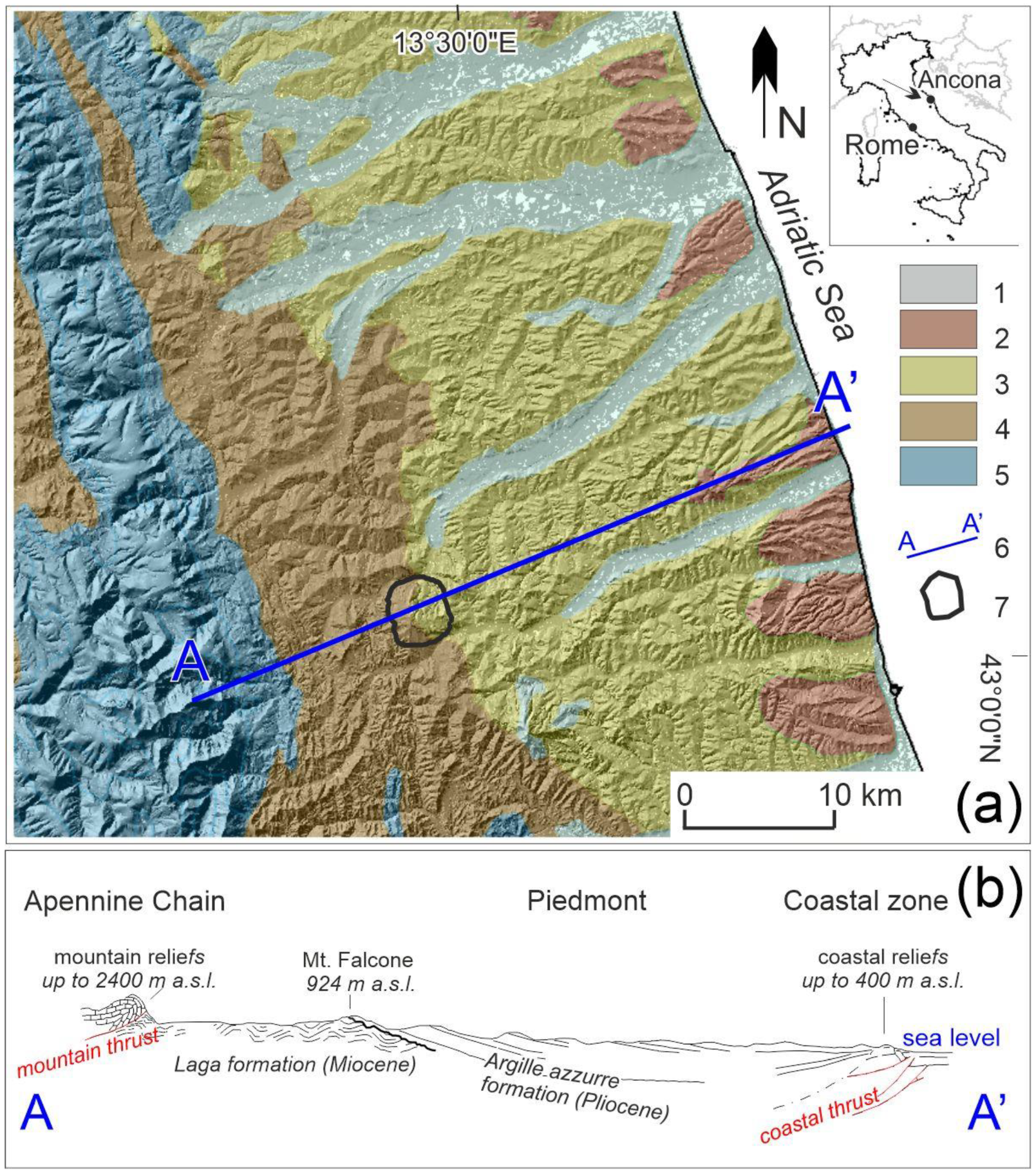
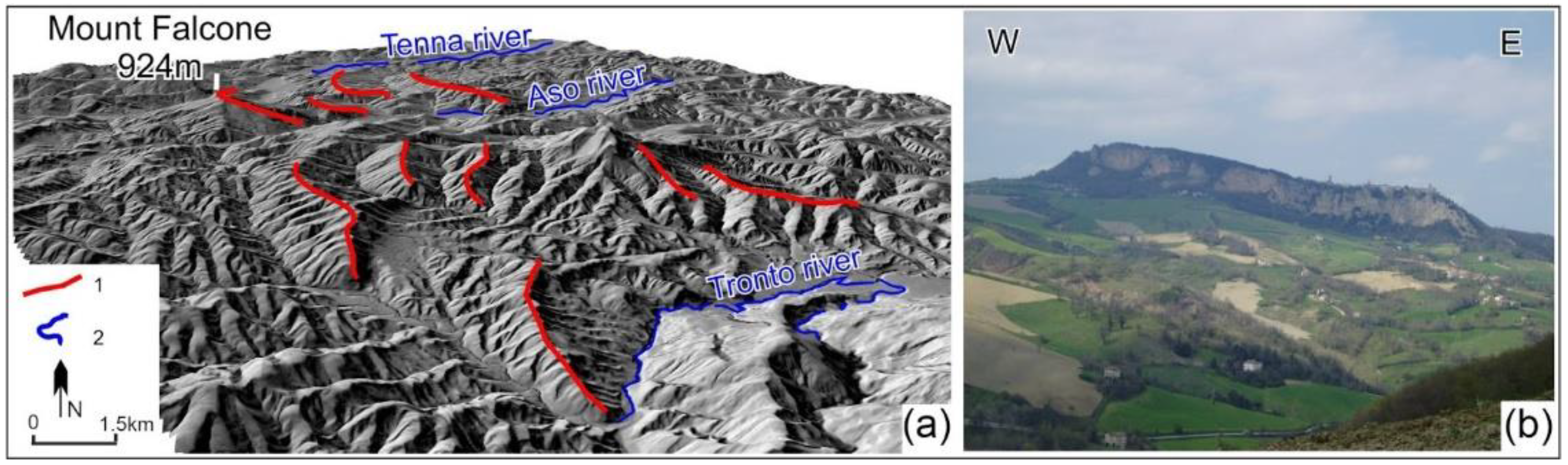
2. Geological and Geomorphological Setting of the Study Area

The study area (around 13 km²) is located east of the Sibillini Mts. Massif (Central Apennines) (Figure 1a). This sector corresponds to a vast sedimentary basin where, starting from the early Pliocene, thick levels of sandstones and conglomerates alternated with pelitic-arenaceous levels are deposited in transgression over a Miocene (Messinian) turbidite bedrock, mainly consisting of alternating arenaceous-pelitic and pelitic-arenaceous levels (Laga formation) [36,37] (Figure 1b,c). The contact between post- and pre-transgressive sediments is marked by an erosion surface approximately parallel to the Miocene levels [32,38]. The area is particularly characterized by the presence of weak levels and ductile deformation zones, corresponding to the weathered levels of the pre-transgressive clayey basement. Such strong weathering is probably due to the long period of immersion of the Messinian sediments as well as the lithostatic charges and the constant presence of water in the arenaceous-calcarenitic aquifer.

The structuring of the pre-transgressive bedrock was essentially carried out in the early Pliocene when, after intense compressive tectonics, east-verging folds and thrusts (the latter emerging or buried) developed within the Messinian and pre-Messinian formations. Pliocene sediments, on the other hand, show a generalized monoclinal setting, linked to the subsequent tectonic uplift that affected the whole area starting from the early Pleistocene [39,40,41]; the strata generally dip between 15° and 20° (Figure 1b).

The resulting landscape, characterized by alignments of strongly asymmetrical and NNW–SSE oriented reliefs, is typical of “cuestas”, with the main element consisting of the Mount Falcone relief (Figure 2a,b). Selective erosion, due to the presence of tough and massive lithotypes (sandstones and conglomerates) overlying less resistant clayey formations, creates steep escarpments between 50 and 300 m on the southwestern flanks.

The monoclinal structure, as a whole, is displaced by direct faults, mainly oriented NNW–SSE and WSW–ENE, the displacement of which can exceed 10 m [36,42]. Micro- and meso-structural analyses carried out on middle Pliocene and upper Pleistocene formations highlighted intense fracturing according to two main joint systems, N70 ± 15, N150 ± 15, and N20 ± 15, N100 ± 10, both compatible with the abovementioned fault systems. In the arenaceous-conglomeratic body of Mount Falcone, a third system of joints, N–S and E–W oriented, has also been observed. The former, dipping W of 70–80°, completely crosses the rigid plate with a spacing of the order of a few tens of meters; the latter, characterized by less frequency and continuity, is found at the edges of the plate itself. The genesis of this third system is attributed to the expansion processes of the relief resulting from the Pleistocene tectonic uplift [43,44] to the passive action of discontinuities developed with the same direction within the pre-transgressive bedrock and, in general, to the high seismicity of the area.

From a geomorphological point of view, the joint systems described above, particularly developed within the arenaceous-conglomeratic body of Mount Falcone (924 m a.s.l.), create strong instability, especially corresponding to the W–SW portion, where the high structural scarp (about 150 m) is affected by retreat processes due to past and ongoing falls and topples (Figure 3). The accumulations of these processes, mainly consisting of pebbles and blocks, constitute an extensive and continuous talus at the base of the slope itself but can also be found further downstream, through rolling and/or passive transport processes induced by slow deformations of debris material; isolated blocks of decametric dimensions were found within the Tenna and Aso riverbeds (north and south of the relief, respectively).

3. Data and Methods

3.1. Geomorphological Approach

The information and the references related to the geological setting of the study area (already included in the text) are included in the caption of Figure 1b.

The detailed study of the morphodynamic processes active in the study area, with particular regard to landslides, was initially carried out following the classical principles of a detailed field geomorphological survey. In the first phase, all the available geological information sources (maps, profiles, stratigraphic sections, stratigraphic logs, etc.) were acquired. The base cartography was the geological map at 1:10,000 scale, which presents an almost complete coverage even at a national level; nevertheless, it is not uniform in symbolism and the legend as it is the product of autonomous regional projects. Furthermore, since this is a relatively old document (about 20 years old), the perimeters and the state of activity of the gravitational processes were updated through a detailed survey, through which soil samples were taken for subsequent geotechnical tests. In this regard, it should be emphasized that specific geotechnical data for outcropping formations are quite rare, and in some cases, it was necessary to use the results of tests conducted on samples taken from the same formations but in different (albeit neighboring) locations.

The synthesis of these surveys, mainly addressing the characterization of the type and evolutionary mechanisms of landslides, is shown in Figure 4a.

From a lithological point of view, the area can be divided into two main sectors, one to the west and one to the east of the relief of Mt. Falcone, consisting of arenaceous and arenaceous-conglomeratic lithotypes associated with a coastal transition environment. In the western sector of the relief, as previously mentioned, the Messinian arenaceous-pelitic and pelitic-arenaceous members of the Laga Formation outcrop with a counter-dip-slope attitude, ranging between 30° and 40° (Figure 4b). Pliocene arenaceous-pelitic and pelitic-arenaceous lithotypes also emerge east of the Mount Falcone relief; the frequency and consistency of the arenaceous levels is, however, less marked as along with the strata inclination (generally dip-slope and between 15–25°). A common feature of some clayey lithotypes is the presence of more or less thick and frequent weathered (weak) levels; these layers, characterized by poor geotechnical properties, are observed mostly in the western sector, within the pelitic-arenaceous member of the Laga formation.

The bedrock is often masked by powerful thicknesses (up to 30 m) of fine colluvial deposits; the greater thicknesses are concentrated corresponding to the numerous minor valleys, which originate from the arenaceous-conglomeratic plate.

The hydrographic network is fairly developed, and because of the low permeability of bedrock and covering soils, the major gullies and streams radially develop from the top of the relief, although there is important tectonic conditioning especially in the lower hierarchical reaches. Concerning water circulation, runoff is limited to a few days/weeks after considerable meteoric events, while the groundwater circulation, due to the predominantly clayey nature of bedrock, is generally limited. However, the presence of widespread perched aquifers within the colluvial deposits, with the water table close to the surface, is a crucial element for the stability of the slopes.

Landslides, as mentioned, are widespread over the area, both for the lithological nature of bedrock and the morphological–structural setting of the slopes, characterized by discrete slope angle and by strata dip often favorable to the activation of gravitational phenomena. The typology of movement is also very highly variable, with falls, topples, flows and slides with different styles and states of activity being present (Figure 4a and Figure 5). Although the stratigraphic setting is favorable to the activation of slides (rotational/planar) particularly on the eastern side, these are less frequent, while flows are dominant; this apparently contradictory aspect can be associated, as described in the following, with the good strength and deformation properties of bedrock and with the presence, on the other hand, of important thicknesses of unconsolidated continental deposits often hosting a perched water table. It is not uncommon, however, to observe complex phenomena characterized by rotational slides in the uppermost portion and flows in the median-terminal one.

The type of movement was mainly attributed on the basis of geomorphological considerations, taking into account size, morphology, typology of material involved, strata dip and damage eventually observed along roads or to infrastructures (Figure 5).

3.2. Numerical Approach

The numerical code used to perform the FoS calculations is the FLAC/Slope v. 8.0. In contrast to other “limit equilibrium” programs, which test several assumed failure surfaces (method of the slices) thus choosing the one with the lowest FoS, FLAC/Slope uses the procedure known as the “strength reduction technique”, a method commonly applied with the Mohr–Coulomb failure criterion in FoS calculations by progressively reducing the shear strength of the material in stages until the slope fails [45,46,47,48,49,50]. The main advantage of a slope stability analysis performed with FLAC/Slope is the possibility to determine a broad variety of failure mechanisms with no prior assumptions concerning their type, shape or location. Moreover, FLAC/Slope is able to combine slip along joints with failure through intact material, thus offering clear advantages in the modelling of jointed rock masses.

The material failure can be defined by either the “Mohr–Coulomb”, the “Modified Hoek–Brown” or the “ubiquitous-joint” plasticity models.

The Mohr–Coulomb model is the conventional model used to represent shear failure in soils and rocks. It assumes that failure is controlled by the maximum shear stress which in turn depends on the normal stress. The solution is obtained by plotting Mohr’s circle for states of stress at failure in terms of the maximum and minimum main stresses: the Mohr–Coulomb failure line is the best straight line tangent to the Mohr’s circles.

The Mohr–Coulomb criterion can be written as

$$\tau =c+{\sigma }_n\tan \varphi$$

(1)

where $\tau$ is the shear stress, $c$ is the cohesion of the material, ${\sigma }_n$ is the normal stress (negative in compression) and $\varphi$ is the angle of friction.

The ubiquitous joint in FLAC/Slope is an anisotropic plasticity model that includes the presence of an oriented weak plane (such as weathering joints) in a Mohr–Coulomb model; failure may occur in either the intact rock, along the weak plane or both and depends on the stress state, the material properties of the rock and weak plane and the orientation of the latter. The failure of the weak plane (ubiquitous joint) may occur by shear, for which the envelope criterion is:

$$\tau =c_j+\tan {\phi }_j{\sigma }_n$$

(2)

or by tension, for which the criterion is:

$${\sigma }_3=-T_j$$

(3)

with:

$$T_j\le \frac{c_j}{\tan {\phi }_j}$$

(4)

where $\tau$ and ${\sigma }_n$ are shear and normal stresses respectively, and ${\sigma }_3$ is the minimum principal stress. $c_j$, ${\phi }_j$ and $T_j$ are the cohesion, friction angle and the tensile strength of the ubiquitous joints, respectively.

Both the Mohr–Coulomb and the ubiquitous-joint models require another parameter, the dilation angle ψ, usually assumed as a fraction of the friction angle and ranging between $\varphi /4$ (very good quality rocks) and 0 (very poor quality rocks) [51,52,53].

The Hoek–Brown failure model for jointed rock masses is defined by the following:

$${\sigma }_1={\sigma }_3+{\sigma }_c{\left(m_b\frac{{\sigma }_3}{{\sigma }_c}+s\right)}^a$$

(5)

where ${\sigma }_1$ and ${\sigma }_3$ (Pa) are the maximum and minimum stresses at failure respectively. Concerning the other parameters, $m_b$ is the value of the Hoek–Brown constant for the rock mass, $s$ and $a$ are constants that depend upon the characteristics of the rock mass and ${\sigma }_c$ (MPa) is the uniaxial compressive strength of the intact rock.

The Modified Hoek–Brown model, sometimes referred to as the “Mhoek model” [54] includes a tensile yield criterion, similar to that used by the Mohr–Coulomb model and can specify a dilation angle ψ. Compared to the original version, the Mhoek model provides a simplified flow rule for both tensile and compressive regions.

The value of ${\sigma }_c$ is usually obtained by laboratory analyses even though several field estimates exist in literature (e.g., Table 1 in [51]).

The constants $m_b$, $s$ and $a$ are usually calculated starting from the evaluation of the geological strength index ($GSI$) of the rock mass [55,56,57,58,59]. The $GSI$ is a system of rock-mass characterization particularly suitable for use in engineering rock mechanics and input into numerical analysis; through a visual assessment of the geological characters of the rock material, it allows the prediction of the rock-mass strength and deformability.

The $GSI$ estimation is carried out using specific charts (see Tables 4 and 5 in [51]): once the index has been evaluated, the constants $s$, $a$ and $m_b$, can be derived with the following equations:

$$s=\exp \left(\frac{GSI-100}{9}\right)\hspace{1em}\hspace{1em}\hspace{1em}\hspace{1em}\mathrm{and}a=0.5\hspace{1em}\hspace{1em}\hspace{1em}\hspace{1em}\mathrm{for}GSI>25$$

(6)

$$s=0\hspace{1em}\hspace{1em}\hspace{1em}\hspace{1em}\mathrm{and}a=0.65-\frac{GSI}{200}\hspace{1em}\hspace{1em}\hspace{1em}\hspace{1em}\mathrm{for}GSI<25$$

(7)

And

$$m_b=m_i\exp \left(\frac{GSI-100}{28}\right)$$

(8)

where $m_i$ is the Hoek–Brown constant for intact rock pieces estimated using $GSI$, ${\sigma }_c$ and the chart of Figure 7 in [51].

The Mhoek model properties can be entered in FLAC/Slope in two different ways; the $s$, $a$ and $m_b$ constants can be input, or $GSI$, $m_i$ and ψ can be entered, and the Hoek–Brown strength properties are calculated automatically from the software.

The FoS calculation model for each cross-section was performed choosing a proper resolution and failure criterion (Mohr–Coulomb or Hoek–Brown) for each numerical mesh. In the case of the arenaceous-conglomeratic body of Mt. Falcone, the ubiquitous-joint model, which considers the characteristics (orientation, tensile strength, cohesion and friction angle) of the previously described joint systems, was used.

Taking into account the type of landslides and the fact that no significant erosion phenomena at the expense of the clayey bedrock are known in the area, the initial state stress, in contrast to other models [59], was assumed as lithostatic as a first approximation. Concerning the presence of water, as it was impossible to implement a discontinuous water table in the models (i.e., to simulate a real perched aquifer), a static water table close to the topographic surface was applied.

The input parameters of the geological formations (

Table 1. Material properties, related to different geological units and implemented within the numerical simulations.

Failure Model	Material Properties (Mohr–Coulomb Method)											Material Properties (Mohr–Coulomb and Modified Hoek–Brown Methods)
Parameter	Friction (φ)					Cohesion (c)						Density (ρ)						Tension (T)							Dilation (ψ)
Units	Deg.					kPa						kg/m3						kPa							Deg.
Range of Values	Min	Mean		Max		Min	Mean			Max		Min		Mean		Max		Min		Mean			Max		Min		Mean		Max
Arenaceous-conglomeratic bedrock (Mount Falcone body)	17	19		20		13,000	15,000			17,000		2050		2335		2620		185		281			377		4.0		6.5		9.0
Mainly arenaceous-pelitic bedrock (Laga formation)	15	17		18		10,500	11,800			13,000		1900		2100		2300		127		147			166		2.0		2.5		3.0
Mainly pelitic-arenaceous bedrock (Laga formation)	14	15		15		5500	6420			7340		1700		1850		2000		56.8		86			11.5		1.0		1.5		2.0
Mainly arenaceous-pelitic bedrock (Argille Azzurre formation)	15	16		17		9500	11,000			12,500		1850		2025		2200		111		132			152		2.0		2.5		3.0
Mainly clayey bedrock (Argille Azzurre formation)	12	20		27		3400	4600			5800		1700		1825		1950		45.9		76.9			108		1.0		1.5		2.0
Weak layer (Laga formation)	n.a	16		n.a		n.a	62.5			n.a		n.a		1650		n.a		n.a		10.5			n.a		0.0		0.0		0.0
Slope and colluvial deposits	17	19		20		8	9			10		1650		1725		1800		0		0			0		n.a		n.a		n.a
Failure Model	Material Properties (Modified Hoek–Brown Method)
Parameter	Geological Strength Index							Hoek–Brown Constant				mb			s						a					σc
Units	(GSI)							(mi)																		(MPa)
Range of Values	Min		Mean		Max			Min	Mean		Max	Min	Mean	Max	Min		Mean		Max		Min	Mean		Max		Min		Mean		Max
Arenaceous-conglomeratic bedrock (Mount Falcone body)	45		55		65			n.a	n.a		n.a	n.a	n.a	n.a	n.a		n.a		n.a		n.a	n.a		n.a		35		45		55
Mainly arenaceous-pelitic bedrock (Laga formation)	40		44		48			18.0	20.0		22.0	2.11	2.77	3.43	0.0012		0.0021		0.0030		0.50	0.50		0.50		29.8		32.3		34.8
Mainly pelitic-arenaceous bedrock (Laga formation)	31		35.5		40			21.0	22.5		24.0	1.78	2.30	2.81	0.0004		0.0008		0.0012		0.50	0.50		0.50		23.5		25.5		27.5
Mainly arenaceous-pelitic bedrock (Argille Azzurre formation)	40		42.5		45			19.0	21.0		23.0	2.22	2.72	3.22	0.0007		0.0015		0.0022		0.50	0.50		0.50		27.4		30.2		32.9
Mainly clayey bedrock (Argille Azzurre formation)	27		31		35			22.0	23.5		25.0	1.62	2.04	2.45	0.0003		0.0005		0.0007		0.50	0.50		0.50		21.6		23.6		25.6
Weak layer (Laga formation)	n.a		20		n.a			n.a	30.0		n.a	n.a	1.72	n.a	n.a		0.0005		n.a		n.a	0.53		n.a		n.a		18		n.a
Slope and colluvial deposits	n.a		n.a		n.a			n.a	n.a		n.a	n.a	n.a	n.a	n.a		n.a		n.a		n.a	n.a		n.a		n.a		n.a		n.a

) were partly obtained from laboratory analyses, performed by professional geologists and provided privately, and partly from direct observations in the field (through $GSI$ evaluation) (Figure 6); a minor number of data were obtained from literature or neighboring territories [51,57,60,61,62,63,64]. Uniform geotechnical properties were assumed throughout the slope, and all the parameters were then used individually or in association with the simulations; in the case of friction angle and cohesion, linked in every failure envelope, the software takes into account only the pair of values specified in the table.

The estimation of the Mohr–Coulomb geotechnical parameters starting from the GSI evaluation was performed by means of the open-source software RocLab v.1.0 (Rockscience Inc., Toronto, ON, Canada) which can plot the Hoek–Brown and the Mohr–Coulomb failure envelopes on the same x–y plane. The results of these calculations are shown in Figure 7.

A shear vs. normal stress plot was obtained for each bedrock unit and for each class of values (min, mean and max).

The range of values (minimum, mean and maximum) was also used for the development of numerical models for each geotechnical cross-section.

4. Results

4.1. Geomorphological Approach

The following numerical analysis was carried out along 10 geotechnical cross-sections: Six are located on the eastern and southeastern sides of the relief of Mount Falcone and four on the western side (Figure 4a). The choice of the location took into account the different morphological–structural conditions of the relief and the results of the geomorphological surveys carried out in the field. To verify all the possible situations observed in the field, the sections were traced to include both portions of the slope affected by gravitational movements and others considered stable.

The geomorphological processes observed along the individual cross-sections can be summarized as follows.

-

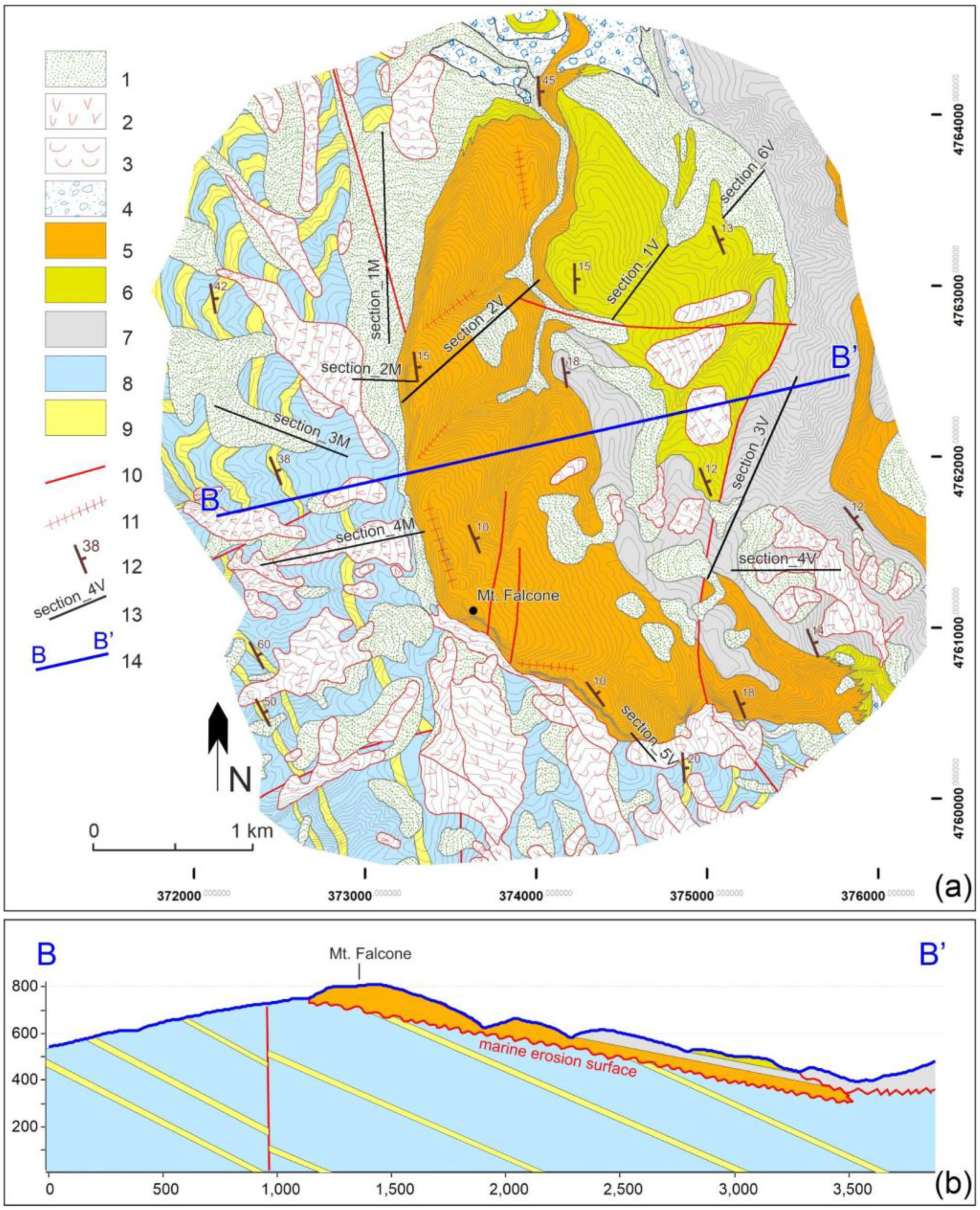
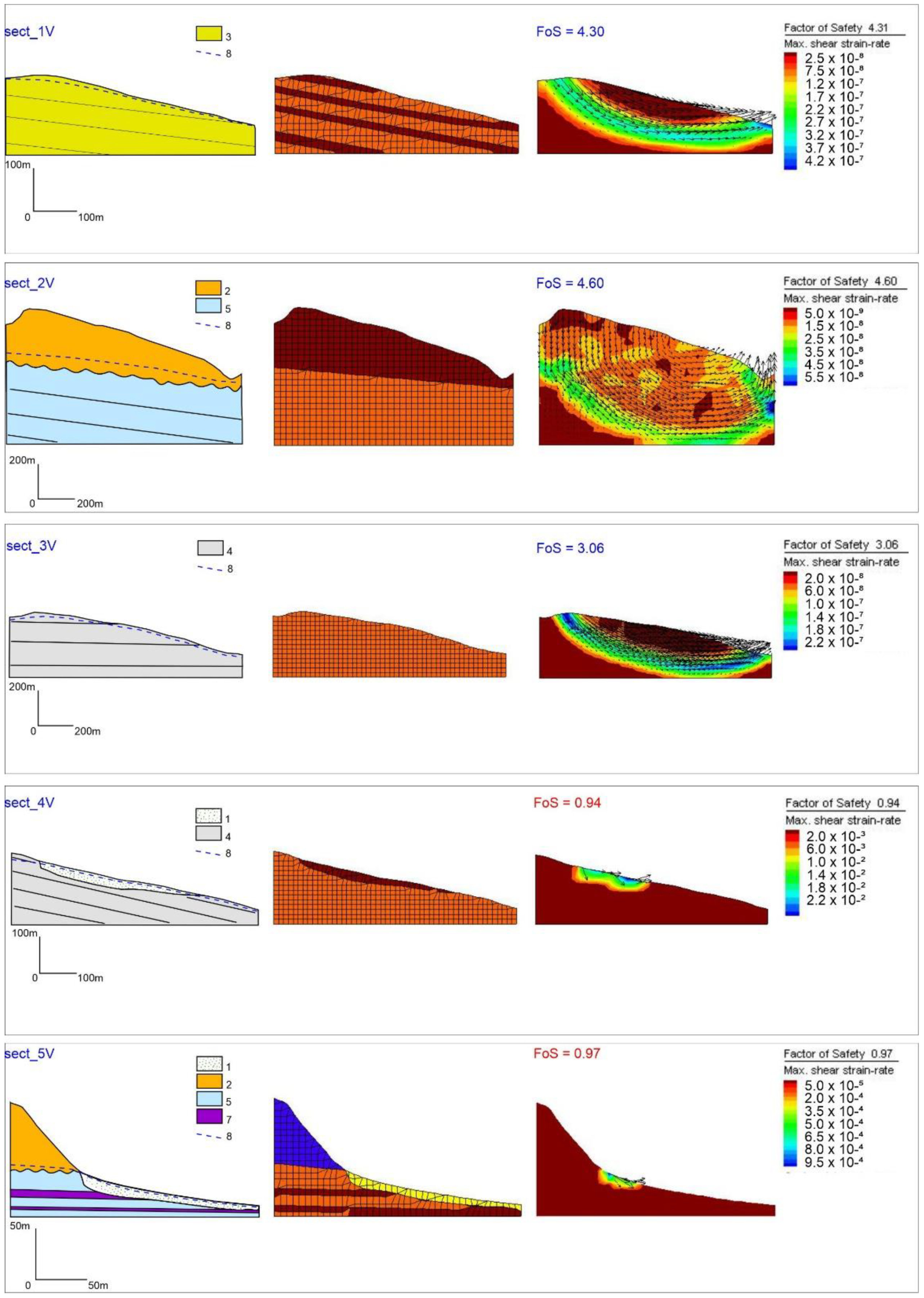
Section 1V. The slope is fairly regular, with a generally mild angle (10–20°). The outcropping bedrock, consisting of the mainly arenaceous-pelitic member of the Argille Azzurre formation, shows a general dip-slope trend with an inclination of about 15° towards E–NE. Almost absent are the continental eluvial–colluvial deposits, which never exceed 1–2 m in thickness and are therefore not shown in the map of Figure 4. The observed geomorphological processes are also not very significant, limited to weak and localized soil erosion processes (sheet and/or rill erosion)

-

Section 2V. This section is traced in the SSW–NNE direction, along the maximum slope and with an angle ranging between 10° and 20° in the first part to over 40° in the final one. The bedrock consists of the mainly arenaceous-conglomeratic body of Mt. Falcone, dipping about 10–15 ° towards ENE. Eluvial–colluvial deposits with low thickness (of a few meters) are present in the central section, but no significant geomorphological processes were detected.

-

Section 3V. The slope, which follows a general SSW–ENE with a moderate angle exceeding 20° only in the lowermost part, is characterized by the presence of the mainly clayey bedrock, dipping 15° towards NE and belonging to the Argille Azzurre formation. In this case, neither appreciable thicknesses of continental deposits nor significant geomorphological processes (mass movements) were observed.

-

Section 4V. This section is traced in a W–E direction, just south of Section 3V. The mainly clayey bedrock (Argille Azzurre formation) here is almost totally covered by thick eluvial–colluvial deposits and is characterized by the presence of several mudflows, which coalesce corresponding to the valley floor. The typology of movement was attributed based on geomorphological considerations such as the material size, the elongated shape of the landslide body (deposited within minor U-shaped valleys), the presence of slight undulations on the surface and the possibility of a concentrated runoff due to the morphology of the slope. The estimate of the landslide depth is, however, uncertain, although it should be linked to the thickness of the continental deposits.

-

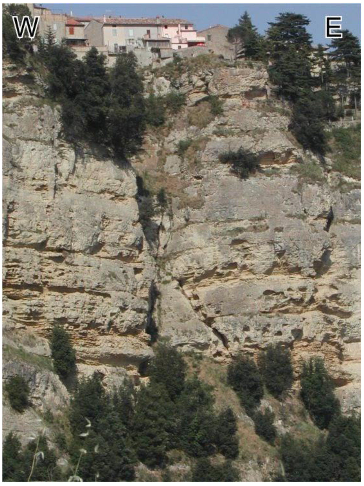
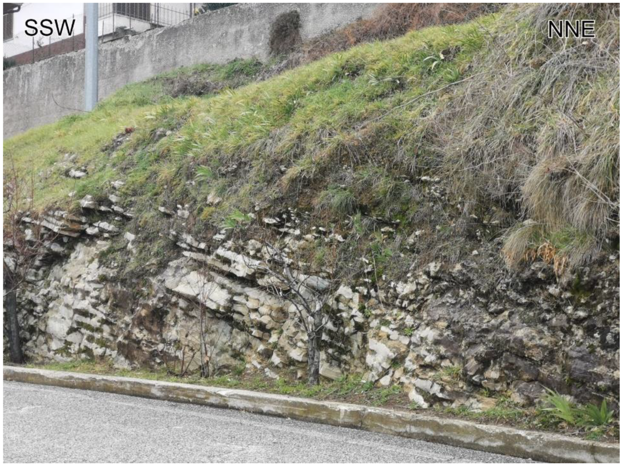
Section 5V. This cross-section is oriented NW–SE and is characterized by the presence of two different litho-technical units: the arenaceous-conglomeratic body of Mt. Falcone in the uppermost part and the pelitic-arenaceous member of the Laga formation in the lowermost one. The morphology of the slope reflects the different nature of the lithotypes with an almost vertical cliff corresponding to the most resistant unit and a gentle slope (15–20°) in the second part of the section. As discussed previously, the Mt. Falcone arenaceous conglomeratic body, especially in this sector, shows a particular joint system, N–S and E–W oriented and associated with tectonic and/or static deformation processes. This unit is affected by rockfalls and toppling phenomena (Figure 3) mainly located along the borders of the plate. The final part of the section, on the other hand, corresponds to the head of an active mudflow roughly WSW–ENE oriented; as with Section 4V this landslide is probably linked to the presence of thick colluvial deposits with a perched water table partially fed by the contact with the permeable arenaceous-conglomeratic plate.

-

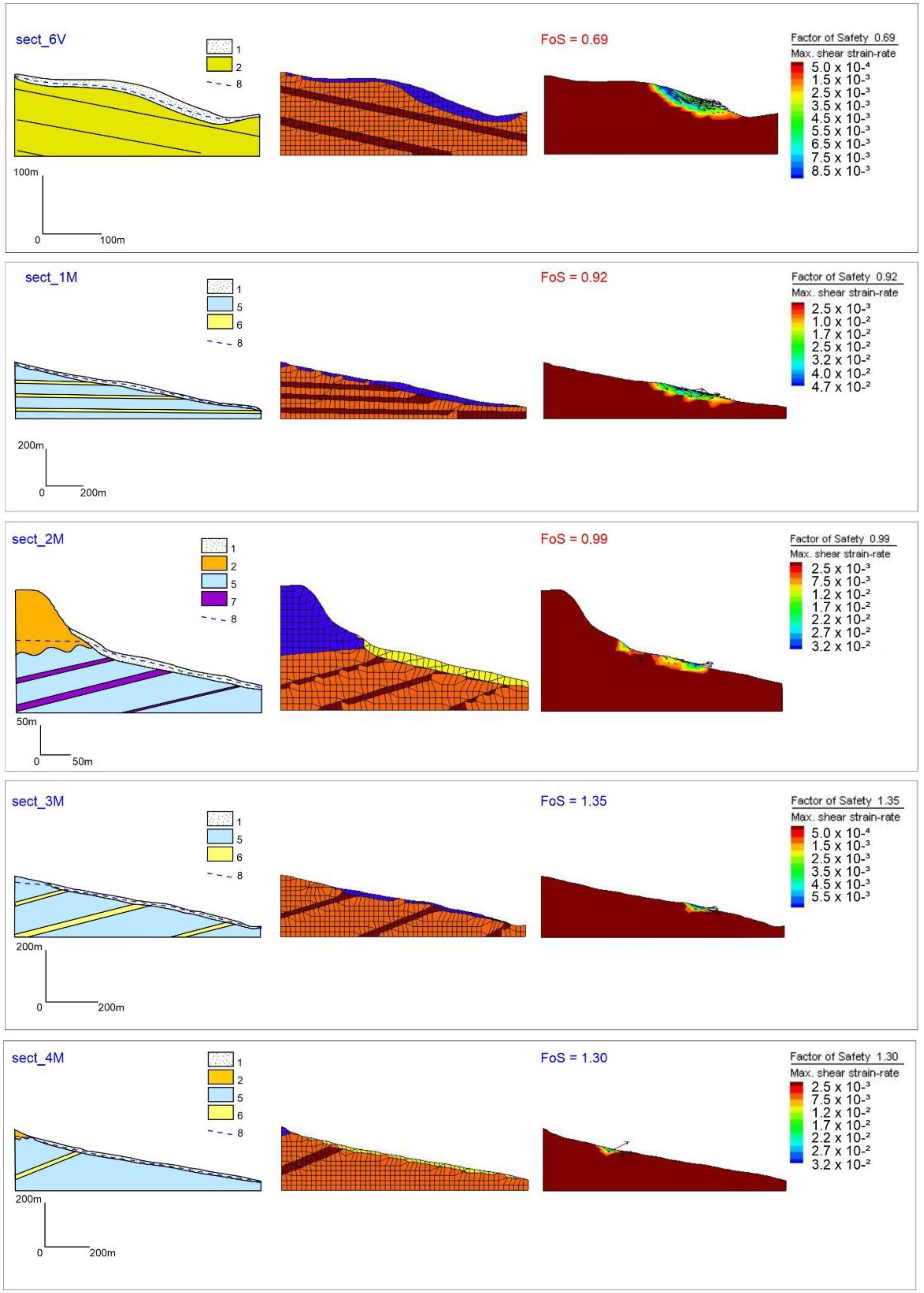
Section 6V. This section is located in the northeastern sector of the study area and crosses, with a NE direction, the arenaceous-pelitic and the clayey members (in the uppermost and lowermost part of the section respectively) of the Argille Azzurre formation, here dipping 13–15° towards NE. The slope angle is moderate and ranges between 10° and 25°. The upper part of the section is characterized by the presence of thick eluvial–colluvial deposits, although no evident geomorphological processes (neither mass movements nor intense soil erosion processes) are visible.

-

Section 1M. This section is traced in the NS direction along a gentle slope (15–20°) almost totally characterized by the presence of thick eluvial–colluvial deposits (10–15 m thick estimated from geomorphological survey and stratigraphic reconstruction); these materials cover a bedrock consisting of alternations of arenaceous-pelitic and pelitic-arenaceous members both belonging to the Laga formation, with apparent horizontal dip. No evident geomorphological processes (landslides or intense soil erosion processes) were observed.

-

Section 2M. Located just south of the previous section, it runs roughly E–W and, similarly to the Section 5V, is characterized by a complex morphology: The first part is strongly conditioned by the presence of the arenaceous conglomeratic body of Mt. Falcone, while the second one, where the pelitic-arenaceous member of the Laga formation is present, shows a low-to-moderate slope (between 15° and 30°). The uppermost part is characterized by rockfalls and toppling phenomena analogous to those observed in Section 5V; the final part corresponds to the head of an active complex landslide (rotational-translational) recognized on the basis of typical morphologies (scarps and counterslopes in the upper portion and minor ridges and scarps in the lower one).

-

Section 3M. This section is traced in a WNW–ESE direction over a slope characterized by a moderate angle (25–30°). Thick colluvial deposits cover the bedrock, visible only in the uppermost part of the section and consisting of alternations of arenaceous and pelitic lithotypes (Laga formation) that dip upslope of 35–40°. No landslides or intense erosion processes were detected.

-

Section 4M. This section is traced in a roughly WSW–ENE direction and, as in Section 3M, runs over a slope characterized by the presence of alternations of arenaceous-pelitic and pelitic-arenaceous lithotypes with the same dip. The geomorphological survey evidenced an active complex landslide (rotational-flow); scarps, counterslopes and minor ridges on a general concave shape are visible, corresponding to the head, while elongated shape and undulations characterize the foot of the landslide. Conditioning and triggering factors can be associated with the presence of colluvial deposits with uncertain thickness and the possible presence of a perched water table fed at the contact with the arenaceous-conglomeratic plate, respectively.

A gravitational movement of greatest scientific and technical interest, given the elevated level of risk connected to the presence of the historical centers mentioned in the previous chapter, is present corresponding to the relief of Mount Falcone (Figure 4). This phenomenon, already studied in the past and verified by numerical modeling both in static and dynamic (seismic) conditions [34,35,58], has been classified as lateral spread and affects, with different intensity, the whole “plate” at the top of the relief. Taking into account the objectives of the present work (mainly addressing the study of medium-to-low depth processes), it was not included in the analysis.

4.2. Numerical Approach

Six simulations were carried out for each section: three using the conditions described above (min, mean and max) and three including the presence of a shallow water table (as often evidenced during field surveys).

The results of the simulations are shown in Figure 8 and Figure 9 and

Table 2. Factor of safety resulting from the numerical modeling and correspondence with field evidence.

Cross- Section	Failure Model	Factor of Safety						In Agreement with the Geomorphological Model
		No Water			Water
		Min	Mean	Max	Min	Mean	Max
Sect_1V	Hoek–Brown	7.46	8.01	8.47	4.30	4.93	5.48	yes
Sect_2V	Hoek–Brown/ Mohr–Coulomb/ Ubiquitous	5.57	5.85	6.09	4.60	4.96	5.22	yes
Sect_3V	Hoek–Brown	5.42	5.86	6.22	3.06	3.51	3.92	yes
Sect_4V	Hoek–Brown/ Mohr–Coulomb	1.28	1.42	1.50	0.94	1.06	1.15	yes
Sect_5V	Hoek–Brown/Mohr–Coulomb/Ubiquitous	1.47	1.62	1.72	0.97	1.08	1.17	only partially
Sect_6V	Hoek–Brown/Mohr–Coulomb	0.96	1.07	1.13	0.71	0.93	0.99	no
Sect_1M	Hoek–Brown/Mohr–Coulomb	1.22	1.38	1.45	0.89	1.01	1.08	no
Sect_2M	Hoek–Brown/Mohr–Coulomb/Ubiquitous	1.28	1.42	1.51	0.96	1.08	1.16	yes
Sect_3M	Hoek–Brown/Mohr–Coulomb	1.49	1.66	1.76	1.35	1.50	1.60	yes
Sect_4M	Hoek–Brown/Mohr–Coulomb/Ubiquitous	1.56	1.74	1.85	1.30	1.46	1.55	no

. More specifically, Figure 8 and Figure 9 show the plots of the simulations that evidenced the lowest FoS values (i.e., worse geotechnical parameters and presence of groundwater); Table 2 includes all the FoS values obtained from the simulations and any correspondences with what was observed in the field (geomorphological model). The same table also reports the failure models used by the software for any simulation.

Sections 1V, 2V and 3V (Figure 8) show high stability in all lithological conditions, with or without the presence of a water table, with FoS values ranging between 3.06 and 8.47 (Table 2).

Nevertheless, the obtained values of FoS as well as shape and depth of the failure surfaces, as evidenced by the model results, are unrealistic and clearly conditioned by the assumed boundary conditions; therefore, for these specific sections, we can only hypothesize a high stability condition and a perfect congruence with the results of the field surveys, which did not show any appreciable phenomenon.

Section 4V (Figure 8) shows a clear instability only in the presence of groundwater, when the FoS drops below 1; in dry conditions the FoS ranges between 1.28 and 1.50, resulting in a condition of moderate stability. The failure surface is located very close to the surface, within the debris cover, while the bedrock, even when dip-sloping, remains almost stable in all conditions. In this case, the model reflects quite faithfully the reality, as a shallow mudflow was observed within a secondary valley filled by colluvial deposits.

Models relating to the section 5V (Figure 8 and Table 2) evidenced highly unstable conditions (FoS between 0.97 and 1.17) only in the presence of water and in dry conditions. As with the previous model, the failure surface is located in the upper portion of the deposits, near the contact with the arenaceous-conglomeratic body of Mount Falcone; the presence of weak levels and ductile deformation zones, as previously described, does not seem to influence the FoS. Unlike the previous case, however, the geomorphological model only partially reflects the numerical one. The field surveys showed the presence of a complex gravitational movement compatible with a slide (probably rotational) in the upper portion of the slope and with a flow in the medium–low portion. The presence of water within the colluvial deposits, observed mainly in autumn and spring, originates at the contact between the overlying arenaceous-conglomeratic body acting as an aquifer and the underlying low-permeability pelitic-arenaceous formation.

Section 6V (Figure 9) shows high instability in all conditions, with and without the presence of water, with FoS between 0.71 and 1.13. Although the stratigraphic setting of the clayey bedrock is favorable to the occurrence of gravitational movements, the failure surface is localized in the medium–low portion of the slope, at the contact between the bedrock itself and the colluvial deposits above. These simulations, however, do not find correspondence in the geomorphological model: any significant phenomenon was observed in the field. This could be linked to an incorrect assessment of the real thicknesses of the deposits, the latter having been estimated in this sector without the aid of geognostic surveys.

The simulations carried out with regard to sections 1M and 2M (Figure 9) yielded similar results, with evidence of instability in the presence of water (FoS between 0.89 and 1.16) and moderate stability in dry conditions (FoS between 1.22 and 1.51). The shear-strain belts are located in positions similar to the previous case, in the middle portion of the slope and inside the colluvial deposits. In these two simulations, the setting of bedrock (i.e., the presence of the weak levels within the pelitic-arenaceous formation in section 2M) does not seem to affect the stability of the slope. The correspondence with the field evidence is different: none in section 1M and good correspondence in section 2M. Taking into account previously mentioned factors, the reason, in the first case, could be found in an incorrect evaluation of the overall thickness of continental deposits.

Finally, sections 3M and 4M (Figure 9) also provided similar results, this time in favor of stability, with the FoS always higher than 1.30 (max = 1.85): The presence of a favorable stratigraphic setting (sub-horizontal or slightly counter dip-slope strata), lower slope angle and limited thickness of colluvial deposits certainly affected the result of the simulations. However, a fair correspondence with the field data was found only in section 3M; in the case of section 4M, on the contrary, a fairly evident mudflow was observed inside the valley, E–W oriented, which originates from the arenaceous-conglomeratic body of Mount Falcone.

By analyzing all the simulations, it is possible to form some general considerations:

• The presence of colluvial deposits of fine grain size and discrete extension and thickness, associated with medium–high slopes angles, generally induces instability conditions;
• In the presence of unconsolidated continental deposits and shallow water table, the FoS tends to reach values close to 1 and consequently activate gravitational movements of discrete extent that are generally not very deep;
• Dip-slope strata and/or clayey bedrock are not sufficient requirements to activate gravitational movements, even in the presence of a water table;
• Complex and medium depth landslides, not highlighted by the simulations, can be explained by the presence of particularly weathered levels within the bedrock neither evidenced during field surveys nor “captured” with typical geognostic surveys.

5. Discussion and Conclusions

Numerical models and, in particular, finite difference programs represent a powerful resource for the study and analysis of gravitational phenomena. Specifically, software such as FLAC/Slope, having characteristic geotechnical parameters of soils and rocks, can be used to carry out important assessments on the stability of the slopes and provide an estimate of the FoS. These assessments can then be used successfully both for purposes related to civil engineering (construction of buildings and infrastructures, effectiveness of slope reinforcement works, etc.) and, more generally, for the assessment of landslide susceptibility of variously sized sectors of the slope. Although they provide numerical results that are indispensable for any type of design and planning, the limits of the models are closely linked to the availability and correctness of the input parameters, which are often missing and limited to single laboratory analyses or estimation through direct observations.

The geomorphological model, based on field observations of the processes active in an area, allows a broader and certainly more articulated evaluation of gravitational phenomena; nevertheless, since it consists of an exclusively qualitative analysis, it cannot provide indices and parameters for performing numerical calculations.

A combined approach that integrates the two models can certainly provide mutual advantages: the ability to confirm and quantify the phenomena observed in the field (the geomorphological model) and to verify and modify model parameters and geometry (the numerical model).

The combined approach, however, when compared to the standard methods (i.e., the statistical methods currently used in Italy for LHA), requires a greater effort both in economic terms and in terms of human resources, since it is necessary to proceed with an update and, often, implementation of the field data. This is all the more onerous in the case of a similar methodology as a standard at the national level where there are large disparities (not only economic) between different regional realities. On the other hand, the possibility of having an updated product that is more functional for professional needs or for the planning of particularly critical areas cannot be separated from an approach that provides for a continuous synthesis between real data and numerical models.

The present study, through this type of approach, provides a more objective evaluation of the mechanisms governing landsliding in a typical geological–structural context, characterized by a monoclinal setting and the presence of lithotypes of different nature and consistency.

More specifically, it was possible to verify that:

• Medium to low GSI values, favorable morphological–structural setting (i.e., dip-slope strata and moderate slope angle) and the presence of a water table are sometimes not evaluated by the numerical model as potentially unstable; on the contrary, they give rise to gravitational phenomena of discrete thickness and extension. This suggests the presence of weak layers at a depth not detectable by generic field surveys or highlighted by specific geognostic investigations;
• The presence of medium–fine colluvial deposits of moderate extension and thickness along medium-to-low slope angles (20–35%) constitutes a predisposing factor to the activation of mass movements (flows as prevalent) with or without the presence of water.

The above considerations could provide further confirmation and perhaps be extended to different morphological–structural contexts, through new detailed surveys and a precise characterization of the buried or outcropping lithotypes.

In conclusion, the proposed approach, which can be defined as semi-quantitative, can be proposed as a valid alternative for LHA in all those countries where specific regulatory indications are absent. The obtained results evidence usefulness and limits of the methods currently used in Italy and, in particular, suggest how a combined use of geomorphological surveys and numerical simulations, pending clearer and universally accepted regulatory indications on the methods to be used for the LHA, seems at the moment the most suitable choice both in economic and safety terms.

References

1. Schuster, R.L.; Highland, L.M. Socioeconomic Impacts of Landslides in the Western Hemisphere; United States Geological Survey: Reston, VA, USA, 2001. [Google Scholar]
2. Winter, M.G.; Shearer, B.; Palmer, D.; Peeling, D.; Harmer, C.; Sharpe, J. The Economic Impact of Landslides and Floods on the Road Network. Procedia Eng. 2016, 143, 1425–1434. [Google Scholar] [CrossRef] [Green Version]
3. Corominas, J.; Van Westen, C.; Frattini, P.; Cascini, L.; Malet, J.-P.; Fotopoulou, S.; Catani, F.; Eeckhaut, M.V.D.; Mavrouli, O.; Agliardi, F.; et al. Recommendations for the quantitative analysis of landslide risk. Bull. Int. Assoc. Eng. Geol. 2013, 73, 209–263. [Google Scholar] [CrossRef]
4. Thiery, Y.; Terrier, M.; Colas, B.; Fressard, M.; Maquaire, O.; Grandjean, G.; Gourdier, S. Improvement of landslide hazard assessments for regulatory zoning in France: STATE–OF–THE-ART perspectives and considerations. Int. J. Disaster Risk Reduct. 2020, 47, 101562. [Google Scholar] [CrossRef]
5. Vandromme, R.; Thiery, Y.; Bernardie, S.; Sedan, O. ALICE (Assessment of Landslides Induced by Climatic Events): A single tool to integrate shallow and deep landslides for susceptibility and hazard assessment. Geomorphology 2020, 367, 107307. [Google Scholar] [CrossRef]
6. Trigila, A.; Iadanza, C.; Bussettini, M.; Lastoria, B. Dissesto Idrogeologico in Italia: Pericolosità e Indicatori Di Rischio, 2018 ed.; ISPRA: Rome, Italy, 2015. [Google Scholar]
7. Guzzetti, F.; Mondini, A.C.; Cardinali, M.; Fiorucci, F.; Santangelo, M.; Chang, K.-T. Landslide inventory maps: New tools for an old problem. Earth Sci. Rev. 2012, 112, 42–66. [Google Scholar] [CrossRef] [Green Version]
8. Bufalini, M.; Materazzi, M.; De Amicis, M.; Pambianchi, G. From Traditional to Modern “ Full Coverage ” Geomorphological Mapping: A Study Case in the Chienti River Basin (Marche Region, Central Italy). J. Maps 2021, 17, 1–12. [Google Scholar] [CrossRef]
9. Cascini, L. Applicability of landslide susceptibility and hazard zoning at different scales. Eng. Geol. 2008, 102, 164–177. [Google Scholar] [CrossRef]
10. Cascini, L. Geotechnics for Urban Planning and Land Use Management. Riv. Ital. Geotech. 2015, 49, 7–62. [Google Scholar]
11. Salvati, P.; Bianchi, C.; Rossi, M.; Guzzetti, F. Landslide Risk to the Population and Its Temporal and Geographical Variation in Italy. In Extreme Events: Observations, Modeling, and Economics; Chavez, M., Ghil, M., Urrutia-Fucugauchi, J., Eds.; John Wiley & Sons: Hoboken, NJ, USA, 2012; Volume 14, pp. 177–194. [Google Scholar]
12. Van Westen, C.J.; van Asch, T.W.J.; Soeters, R. Landslide Hazard and Risk Zonation—Why Is It Still so Diffi-cult? Bull. Eng. Geol. Environ. 2006, 65, 167–184. [Google Scholar] [CrossRef]
13. Thiery, Y.; Terrier, M. Évaluation de l’aléa Glissements de Terrain: État de l’art et Perspectives Pour La Car-tographie Réglementaire En France. Rev. Française Géotechnique 2018, 156, 3. [Google Scholar] [CrossRef]
14. Aleotti, P.; Chowdhury, R. Landslide hazard assessment: Summary review and new perspectives. Bull. Int. Assoc. Eng. Geol. 1999, 58, 21–44. [Google Scholar] [CrossRef]
15. Galli, M.; Ardizzone, F.; Cardinali, M.; Guzzetti, F.; Reichenbach, P. Comparing landslide inventory maps. Geomorphology 2008, 94, 268–289. [Google Scholar] [CrossRef]
16. Soeters, R.; van Westen, C.J. Slope Instability Recognition, Analysis, and Zonation. In Landslides, Investigation and Mitigation; Turner, A.K., Schuster, R.L., Eds.; Special Report; National Research Council, Transportation Research Board: Washington, DC, USA, 1996; Volume 247, pp. 129–147. [Google Scholar]
17. Cotecchia, F.; Santaloia, F.; Lollino, P.; Vitone, C.; Pedone, G.; Bottiglieri, O. From a phenomenological to a geomechanical approach to landslide hazard analysis. Eur. J. Environ. Civ. Eng. 2016, 20, 1004–1031. [Google Scholar] [CrossRef]
18. Guzzetti, F.; Carrara, A.; Cardinali, M.; Reichenbach, P. Landslide Hazard Evaluation: A Review of Current Techniques and Their Application in a Multi-Scale Study, Central Italy. Geomorphology 1999, 31, 181–216. [Google Scholar] [CrossRef]
19. Nandi, A.; Shakoor, A. A GIS-Based Landslide Susceptibility Evaluation Using Bivariate and Multivariate Sta-tistical Analyses. Eng. Geol. 2010, 110, 11–20. [Google Scholar] [CrossRef]
20. Pourghasemi, H.R.; Kerle, N. Random Forests and Evidential Belief Function-Based Landslide Susceptibility Assessment in Western Mazandaran Province, Iran. Environ. Earth Sci. 2016, 75, 185. [Google Scholar] [CrossRef]
21. Chen, X.; Chen, W. GIS-Based Landslide Susceptibility Assessment Using Optimized Hybrid Machine Learn-ing Methods. Catena 2021, 196, 104833. [Google Scholar] [CrossRef]
22. Pourghasemi, H.R.; Mohammady, M.; Pradhan, B. Landslide Susceptibility Mapping Using Index of Entropy and Conditional Probability Models in GIS: Safarood Basin, Iran. Catena 2012, 97, 71–84. [Google Scholar] [CrossRef]
23. Barla, G. Numerical Modeling of Deep-Seated Landslides Interacting with Man-Made Structures. J. Rock Mech. Geotech. Eng. 2018, 10, 1020–1036. [Google Scholar] [CrossRef]
24. Cuomo, S. New Advances and Challenges for Numerical Modeling of Landslides of the Flow Type. Procedia Earth Planet. Sci. 2014, 9, 91–100. [Google Scholar] [CrossRef] [Green Version]
25. Fustos, I.; Abarca-del-Río, R.; Mardones, M.; González, L.; Araya, L.R. Rainfall-Induced Landslide Identifica-tion Using Numerical Modelling: A Southern Chile Case. J. S. Am. Earth Sci. 2020, 101, 102587. [Google Scholar] [CrossRef]
26. Marcato, G.; Mantovani, M.; Pasuto, A.; Zabuski, L.; Borgatti, L. Monitoring, Numerical Modelling and Hazard Mitigation of the Moscardo Landslide (Eastern Italian Alps). Eng. Geol. 2012, 128, 95–107. [Google Scholar] [CrossRef]
27. Viero, A.; Kuraoka, S.; Borgatti, L.; Breda, A.; Marcato, G.; Preto, N.; Galgaro, A. Numerical Models for Plan-ning Landslide Risk Mitigation Strategies in Iconic but Unstable Landscapes: The Case of Cinque Torri (Dolomites, Italy). Eng. Geol. 2018, 240, 163–174. [Google Scholar] [CrossRef]
28. Griffiths, D.V.; Lu, N. Unsaturated Slope Stability Analysis with Steady Infiltration or Evaporation Using Elasto-Plastic Finite Elements. Int. J. Numer. Anal. Methods Geomech. 2005, 29, 249–267. [Google Scholar] [CrossRef]
29. Sorbino, G.; Sica, C.; Cascini, L. Susceptibility Analysis of Shallow Landslides Source Areas Using Physically Based Models. Nat. Hazards 2010, 53, 313–332. [Google Scholar] [CrossRef]
30. Formetta, G.; Rago, V.; Capparelli, G.; Rigon, R.; Muto, F.; Versace, P. Integrated Physically Based System for Modeling Landslide Susceptibility. Procedia Earth Planet. Sci. 2014, 9, 74–82. [Google Scholar] [CrossRef] [Green Version]
31. Centamore, E.; Nisio, S. Effects of Uplift and Tilting in the Central-Northern Apennines (Italy). Quat. Int. 2003, 101–102, 93–101. [Google Scholar] [CrossRef]
32. Gentili, B.; Pambianchi, G.; Aringoli, D.; Materazzi, M.; Giacopetti, M. Pliocene-Pleistocene Geomorphological Evolution of the Adriatic Side of Central Italy. Geol. Carpathica 2017, 68, 6–18. [Google Scholar] [CrossRef] [Green Version]
33. Itasca. FLAC—Fast Lagrangian Analysis of Continua, Version 8.0.; Itasca Consulting Group Inc., Ed.; Itasca Consulting Group, Inc.: Minneapolis, MN, USA, 2016. [Google Scholar]
34. Crescenti, U.; Sciarra, N.; Gentili, B.; Pambianchi, G. Modeling of Complex Deep-Seated Mass Movements in the Central-Southern Marches (Central Italy). In Landslides; Rybář, J., Stemberk, J., Wagner, P., Eds.; Balkema: Lisse, The Netherlands, 2002; pp. 149–155. [Google Scholar] [CrossRef]
35. Aringoli, D.; Gentili, B.; Materazzi, M. Mass movements in Adriatic central Italy: Activation and evolutive control factors. In Landslides: Causes, Types and Effects; Nova Science Publishers, Inc.: New York, NY, USA, 2010; pp. 1–71. [Google Scholar]
36. Cantalamessa, G.; Centamore, E.; Chiocchini, U.; Colalongo, M.L.; Micarelli, A.; Nanni, T.; Pasini, G.; Potetti, M.; Ricci Lucchi, F.; Cristallini, C.; et al. Il Plio-Pleistocene Delle Marche. Studi Geologici Camerti (Special Volume “La Geologia delle Marche”) 1986, 61–81. Available online: https://www.semanticscholar.org/paper/Il-Plio-Pleistocene-delle-Marche.-Cantalamessa-Centamore/1f38e45fcff286816bcdedfb2da9ea0146477f9d (accessed on 20 March 2021).
37. Ori, G.G.; Serafini, G.; Visentin, C.; Lucchi, F.R.; Casnedi, R.; Colalongo, M.L.; Mosna, S. The Pliocene-Pleistocene Adriatic Foredeep (Marche and Abruzzo, Italy): An Integrated Approach to Surface and Subsur-face Geology. In 3rd EAPG Conference, Adriatic Foredeep Field Trip Guide Book; EAPG and AGIP: Florence, Italy, 1991; pp. 26–30. [Google Scholar]
38. Gentili, B.; Materazzi, M.; Pambianchi, G.; Scalella, G.; Aringoli, D.; Cilla, G.; Farabollini, P. The Slope Deposits of the Ascensione Mount (Southern Marche, Italy). Geogr. Fis. Din. Quat. 1998, 21, 205–214. [Google Scholar]
39. Cantalamessa, G.; Di Celma, C. Sequence Response to Syndepositional Regional Uplift: Insights from High-Resolution Sequence Stratigraphy of Late Early Pleistocene Strata, Periadriatic Basin, Central Italy. Sediment. Geol. 2004, 164, 283–309. [Google Scholar] [CrossRef]
40. Buccolini, M.; Bufalini, M.; Coco, L.; Materazzi, M.; Piacentini, T. Small Catchments Evolution on Clayey Hilly Landscapes in Central Apennines and Northern Sicily (Italy) since the Late Pleistocene. Geomorphology 2020, 363, 107206. [Google Scholar] [CrossRef]
41. Ambrosetti, P.; Carraro, F.; Deiana, G.; Dramis, F. Il Sollevamento Dell’Italia Centrale Tra Il Pleistocene Infe-riore e Il Pleistocene Medio. P.F. Geodin. 1982, 513, 219–223. [Google Scholar]
42. Buccolini, M.; Gentili, B.; Materazzi, M.; Piacentini, T. Late Quaternary Geomorphological Evolution and Ero-sion Rates in the Clayey Peri-Adriatic Belt (Central Italy). Geomorphology 2010, 116, 145–161. [Google Scholar] [CrossRef]
43. Wise, D.U.; Funiciello, R.; Parotto, M.; Salvini, F. Topographic Lineament Swarms: Clues to Their Origin from Domain Analysis of Italy. Bull. Geol. Soc. Am. 1985, 96, 952–967. [Google Scholar] [CrossRef]
44. Calamita, F. Extensional Mesostructures in Thrust Shear Zone: Example from the Umbro-Marchean Appen-nines. Boll. Soc. Geol. Ital. 1991, 110, 649–660. [Google Scholar]
45. Zienkiewicz, C.; Humpheson, C.; Lewis, R.W. Associated and Non-Associated Visco-Plasticity and Plasticity in Soil Mechanics. Geotechnique 1975, 25, 671–689. [Google Scholar] [CrossRef]
46. Naylor, D.J. Finite Elements and Slope Stability. In Numerical Methods in Geomechanics; Springer: Dordrecht, The Netherlands, 1982; Volume 8, pp. 229–244. [Google Scholar]
47. Matsui, T.; San, K.-C. Finite Element Slope Stability Analysis by Shear Strength Reduction Technique. Soils Found. 1992, 32, 59–70. [Google Scholar] [CrossRef] [Green Version]
48. Ugai, K. A Method of Calculation of Total Factor of Safety of Slopes by Elasto-Plastic FEM. Soils Found. 1989, 29, 190–195. [Google Scholar] [CrossRef] [Green Version]
49. Ugai, K.; Leshchinsky, D. Three-Dimensional Limit Equilibrium and Finite Element Analyses: A Comparison of Results. Soils Found. 1995, 35, 1–7. [Google Scholar] [CrossRef]
50. Dawson, E.M.; Roth, W.H.; Drescher, A. Slope Stability Analysis by Strength Reduction. Geotechnique 1999, 49, 835–840. [Google Scholar] [CrossRef]
51. Hoek, E.; Brown, E.T. Practical Estimates of Rock Mass Strength. Int. J. Rock Mech. Min. Sci. 1997, 34, 1165–1186. [Google Scholar] [CrossRef]
52. Alejano, L.R.; Alonso, E. Considerations of the Dilatancy Angle in Rocks and Rock Masses. Int. J. Rock Mech. Min. Sci. 2005, 42, 481–507. [Google Scholar] [CrossRef]
53. Zhao, X.G.; Cai, M. A Mobilized Dilation Angle Model for Rocks. Int. J. Rock Mech. Min. Sci. 2010, 47, 368–384. [Google Scholar] [CrossRef]
54. Cundall, P.A.; Carranza-Torres, C.; Hart, R.D. A New Constitutive Model Based on the Hoek-Brown Criteri-on. FLAG Numer. Model. In FLAC and Numerical Modeling in Geomechanics, Proceedings of the third International Flac Symposium, Sudbury, ON, Canada, 21–24 October 2003; Balkema: Lisse, The Netherlands, 2003. [Google Scholar]
55. Hoek, E. Strength of Rock and Masses. ISRM New J. 1994, 2, 4–16. [Google Scholar]
56. Hoek, E.; Kaiser, P.K.; Bawden, W.F. Support of Underground Excavations in Hard Rock. Environ. Eng. Geosci. 1996, 2, 609–615. [Google Scholar] [CrossRef]
57. Marinos, P.; Marinos, V.; Hoek, E. Geological Strength Index (GSI): A characterization tool for assessing engineering properties for rock masses. In Proceedings of International Workshop on Rock Mass Classification for Underground Mining; Mark, C., Pakalnis, R., Tuchman, R.J., Eds.; Taylor and Francis Group: Madrid, Spain; London, UK, 2007; pp. 87–94. [Google Scholar] [CrossRef]
58. Aringoli, D.; Buccolini, M.; Coco, L.; Dramis, F.; Farabollini, P.; Gentili, B.; Giacopetti, M.; Materazzi, M.; Pambianchi, G. The Effects of In-Stream Gravel Mining on River Incision: An Example from Central Adriatic Italy. Zeitschrift Geomorphol. 2015, 59, 95–107. [Google Scholar] [CrossRef]
59. Lollino, P.; Cotecchia, F.; Elia, G.; Mitaritonna, G.; Santaloia, F. Interpretation of landslide mechanisms based on numerical modelling: Two case-histories. Eur. J. Environ. Civ. Eng. 2016, 20, 1032–1053. [Google Scholar] [CrossRef]
60. Hoek, E.; Marinos, P.; Benissi, M. Applicability of the Geological Strength Index (GSI) Classification for Very Weak and Sheared Rock Masses. The Case of the Athens Schist Formation. Bull. Eng. Geol. Environ. 1998, 57, 151–160. [Google Scholar] [CrossRef]
61. Marinos, P.; Hoek, E. Estimating the Geotechnical Properties of Heterogeneous Rock Masses Such as Flysch. Bull. Eng. Geol. Environ. 2001, 60, 85–92. [Google Scholar] [CrossRef]
62. Budetta, P.; Nappi, M. Heterogeneous Rock Mass Classification by Means of the Geological Strength Index: The San Mauro Formation (Cilento, Italy). Bull. Eng. Geol. Environ. 2011, 70, 585–593. [Google Scholar] [CrossRef]
63. Stück, H.; Koch, R.; Siegesmund, S. Petrographical and Petrophysical Properties of Sandstones: Statistical Analysis as an Approach to Predict Material Behaviour and Construction Suitability. Environ. Earth Sci. 2013, 69, 1299–1332. [Google Scholar] [CrossRef] [Green Version]
64. Cantalamessa, G.; Centamore, E.; Didaskalou, P.; Micarelli, A.; Napoleone, G.; Potetti, M. Elementi Di Correlazione Nella Successione Marina Plio-Pleistocenica Del Bacino Periadriatico Marchigiano. Stud. Geol. Camerti 2002, 1, 33–49. [Google Scholar]
Figure 1. (a) Schematic geological map of the study sector: 1—main continental deposits (Pleistocene–Holocene); 2—sands and conglomerates (Pliocene–Pleistocene); 3—clays and sands (Pliocene–Pleistocene); 4—arenaceous-marly-clayey turbidites (late Miocene); 5—limestones, marly limestones and marls (early Jurassic–Oligocene); 6—trace of cross-section shown in Figure 1b; 7—study area (see Figure 4). (b) Schematic geological cross-section from the Apennine chain to the Adriatic Sea, modified from [42].
Land 10 00624 g001
Figure 2. (a) 3D digital elevation model of the study sector: 1—edge of cuesta; 2—river. (b) The arenaceous-conglomeratic body of Mount Falcone.
Land 10 00624 g002
Figure 3. Open fractures and toppling phenomena affecting the arenaceous plate of Mount Falcone.
Land 10 00624 g003
Figure 4. (a). Geological and geomorphological map of the study area: 1—slope and colluvial deposits (Holocene); 2—rotational and planar slides (Holocene); 3—flows (Holocene); 4—old and recent fluvial deposits (Pleistocene–Holocene); 5—arenaceous-conglomeratic bedrock (Mount Falcone body—Middle Pliocene); 6—mainly arenaceous-pelitic bedrock (Argille Azzure Formation—Middle Pliocene); 7—mainly clayey bedrock (Argille Azzure Formation—Middle Pliocene); 8—mainly pelitic-arenaceous bedrock (Laga formation—Late Messinian); 9—mainly arenaceous-pelitic bedrock (Laga formation—Late Messinian); 10—main faults; 11—gravitational trench; 12—strata attitude; 13—trace of cross-section used for the numerical simulation; 14—trace of geological cross-section described in (b).
Land 10 00624 g004
Figure 5. Typical landslides in the study area. (a) Rotational slide affecting clayey bedrock and (b) consequences on the road conditions; (c) example of earthflow involving fine slope deposits and (d) secondary road deformed by a landslide.
Land 10 00624 g005
Figure 6. Arenaceous-conglomeratic bedrock outcropping on the eastern side of the relief of Mount Falcone.
Land 10 00624 g006
Figure 7. Shear vs. normal stress plots of Hoek–Brown and Mohr–Coulomb failure envelopes, obtained for each litho-technical unit and different range of values.
Land 10 00624 g007
Figure 8. Results of numerical simulation (Sections 1V, 2V, 3V, 4V, 5V). From left to right: geotechnical cross-section, mesh and model result. 1—slope and colluvial deposits; 2—arenaceous-conglomeratic bedrock; 3—arenaceous-pelitic and pelitic-arenaceous bedrock; 4—mainly clayey bedrock; 5—mainly pelitic-arenaceous bedrock; 6—mainly arenaceous-pelitic bedrock; 7—weak layer/ductile deformation zone; 8—water table.
Land 10 00624 g008
Figure 9. Results of numerical simulation (Sections 6V, 1M, 2M, 3M, 4M). From left to right: geotechnical cross-section, mesh and model result. 1—slope and colluvial deposits; 2—arenaceous-conglomeratic bedrock; 3—arenaceous-pelitic and pelitic-arenaceous bedrock; 4—mainly clayey bedrock; 5—mainly pelitic-arenaceous bedrock; 6—mainly arenaceous-pelitic bedrock; 7—weak layer/ductile deformation zone; 8—water table.
Land 10 00624 g009