Article

The Multiscale Monitoring of Peatland Ecosystem Carbon Cycling in the Middle Taiga Zone of Western Siberia: The Mukhrino Bog Case Study

1
Laboratory of Ecosystem-Atmosphere Interactions of the Mire-Forest Landscapes, Yugra State University, 628012 Khanty-Mansiysk, Russia
2
Laboratory of Physics of Climatic Systems, Institute of Monitoring of Climatic and Ecological Systems SB RAS, 634055 Tomsk, Russia
3
Bioeconomy and Environment, Natural Resources Institute Finland, FI-00790 Helsinki, Finland
4
Ecohydrology Department, KWR Water Research Institute, 3430 BB Nieuwegein, The Netherlands
5
Institute of Atmospheric and Earth System Research, Department of Physics, University of Helsinki, 00014 Helsinki, Finland
6
Institute of Atmospheric and Earth System Research, Department of Forest Sciences, University of Helsinki, 00014 Helsinki, Finland
7
Department of Physical Geography, Utrecht University, 3584 CB Utrecht, The Netherlands
8
Institute of Earth Sciences, University of Tyumen, 625002 Tyumen, Russia
*
Author to whom correspondence should be addressed.
Submission received: 25 June 2021 / Revised: 3 August 2021 / Accepted: 3 August 2021 / Published: 6 August 2021
(This article belongs to the Special Issue Peatland Ecosystem)

Abstract

:
The peatlands of the West Siberian Lowlands, comprising the largest pristine peatland area of the world, have not previously been covered by continuous measurement and monitoring programs. The response of peatlands to climate change occurs over several decades. This paper summarizes the results of peatland carbon balance studies collected over ten years at the Mukhrino field station (Mukhrino FS, MFS) operating in the Middle Taiga Zone of Western Siberia. A multiscale approach was applied for the investigations of peatland carbon cycling. Carbon dioxide fluxes at the local scale studied using the chamber method showed net accumulation with rates from 110, to 57.8 gC m−2 at the Sphagnum hollow site. Net CO2 fluxes at the pine-dwarf shrubs-Sphagnum ridge varied from negative (−32.1 gC m−2 in 2019) to positive (13.4 gC m−2 in 2017). The cumulative May-August net ecosystem exchange (NEE) from eddy-covariance (EC) measurements at the ecosystem scale was −202 gC m−2 in 2015, due to the impact of photosynthesis of pine trees which was not registered by the chamber method. The net annual accumulation of carbon in the live part of mosses was estimated at 24–190 gC m−2 depending on the Sphagnum moss species. Long-term carbon accumulation rates obtained by radiocarbon analysis ranged from 28.5 to 57.2 gC m−2 yr−1, with local extremes of up to 176.2 gC m−2 yr−1. The obtained estimates of various carbon fluxes using EC and chamber methods, the accounting for Sphagnum growth and decomposition, and long-term peat accumulation provided information about the functioning of the peatland ecosystems at different spatial and temporal scales. Multiscale carbon flux monitoring reveals useful new information for forecasting the response of northern peatland carbon cycles to climatic changes.

1. Introduction

Several modern studies have focused on climate change-related issues and anthropogenic impacts on the environment [1,2,3,4]. Increasing average atmospheric temperatures are strongly related to the concentration of greenhouse gases (GHGs), such as methane and carbon dioxide. Pristine peatland ecosystems play an important role in the global carbon balance by carbon sequestration and controlling GHG emissions [5,6], thus regulating the atmospheric composition and climate. Peatlands occupy only ~3% of the land surface globally but have accumulated an equivalent of half of the atmosphere’s carbon as peat [7,8]. Even small changes in their functioning may, therefore, cause a disbalance in the biosphere. One of the most waterlogged areas in the world is the West Siberian Lowland (WSL), where peatlands cover 592,440 km2 and store ~3.2% (70.21 Pg C) of all terrestrial carbon [9].
The gaseous exchange between the atmosphere and peatlands is governed by the photosynthetic uptake of CO2 from the atmosphere and by soil and vegetation respiration losses of CO2. The difference between them is known as the net ecosystem exchange (NEE) of CO2 [10,11,12,13]. The other major gaseous emission of carbon (C) into the atmosphere is accounted for by methane (CH4), which is produced via the anoxic decay of organic matter [14]. According to IPCC estimates [15], the contribution of natural mires into total natural methane emissions ranges between 61 and 82%. The intensity of GHG fluxes from peat deposits is controlled by different factors, including hydrological and thermal regimes [16,17,18,19,20,21].
Climatic changes occur on a timescale of a decade and longer, thus requiring long-term monitoring to detect their effect on ecosystems. Continuous monitoring helps to detect ongoing changes in the peatland (biodiversity, net primary production, GHG emission, and carbon and nitrogen sequestration rates) and to define the role of external factors (climate, hydrology) affecting the peatland ecosystems [22].
Despite the global importance of peatlands, there are limited long-term monitoring data to quantify the functioning of the extensive peatlands of WSL, which are not covered by continuous comprehensive monitoring programs such as Fluxnet [23].
Assessments of the representativeness of the pan-Arctic eddy-covariance site network [24] showed that large parts of Siberia and patches of Canada are under-represented in carbon balance studies [25]. Only a few long-term sites with monitoring of GHG are available in Western Siberia, including the ZOTTO tall tower with a supporting eddy-covariance network along the Yenisei river [26] and the Japan-Russia Siberian Tall Tower Inland Observation Network located in the taiga, steppe, and wetland biomes of Siberia [27].There automated chamber observations of methane and carbon dioxide fluxes [28] and manual routine studies of peatland carbon balance [29] and mire water chemistry have been carried out [30].
The most intense field studies of the West Siberian peatlands are related to the investigation of methane fluxes from inland waters [31], shallow lakes [32], floodplains [33] and peatlands [34], and trace element distribution in snow deposits [35].
Because West Siberian peatlands constitute most of all peatlands on the Eurasian continent [8], the establishment of long-term records of GHG and water vapor exchange between peatlands and the atmosphere in this area under specific hydroclimatological and geological settings are essential. Intact peatlands act as significant sinks and stores of carbon and water, play a vital role as climate-regulators on a global and regional scale, and are safe-havens for unique biodiversity [22,36].
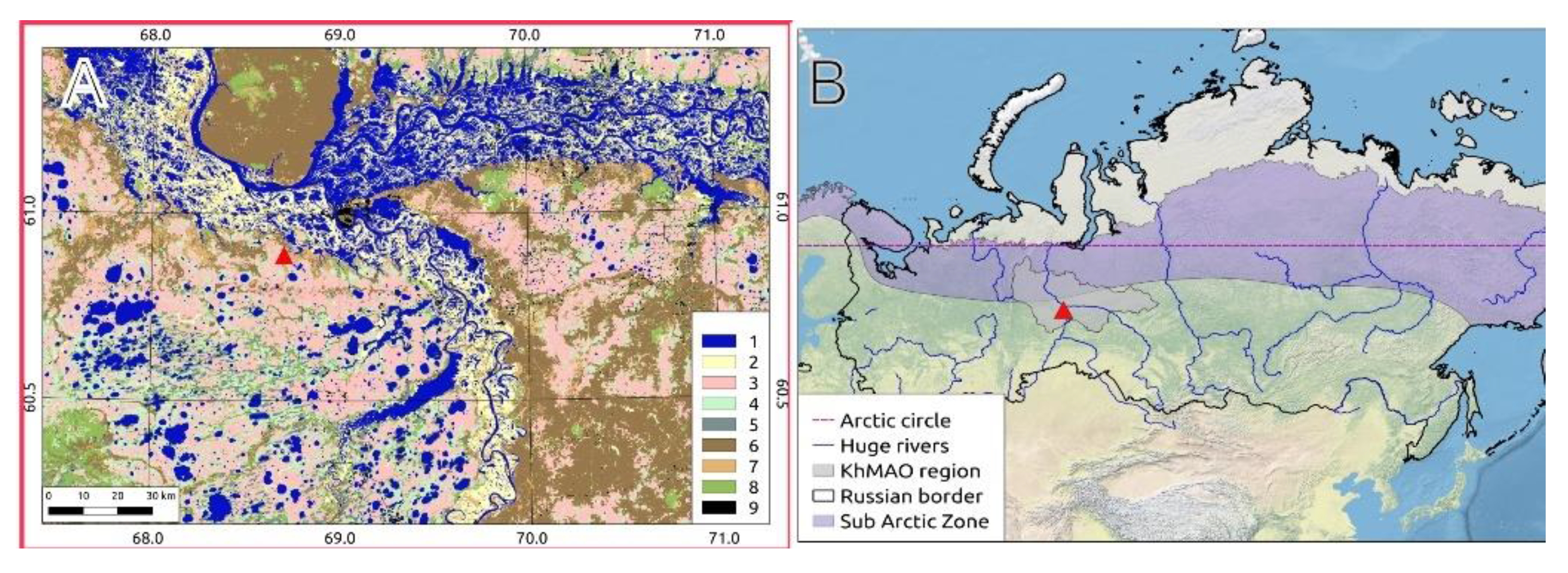
The Mukhrino field station (Mukhrino FS, MFS) was established in 2009 with the aim of filling this shortcoming in peatland data records from the West Siberian middle taiga zone. The research is focused on climate change, carbon cycling, and biodiversity.
A multiscale approach was applied for the investigation of peatland carbon cycling. Vegetation net productivity determined from Sphagnum growth rates was used to estimate the input carbon of the ecosystem during the snow-free period. The decomposition rate of plant remains characterizes the relative activity of the microbial transformation of peat at various ecological conditions. The resulting carbon dioxide fluxes at the local scale were studied using the chamber method. Eddy-covariance techniques summarized CO
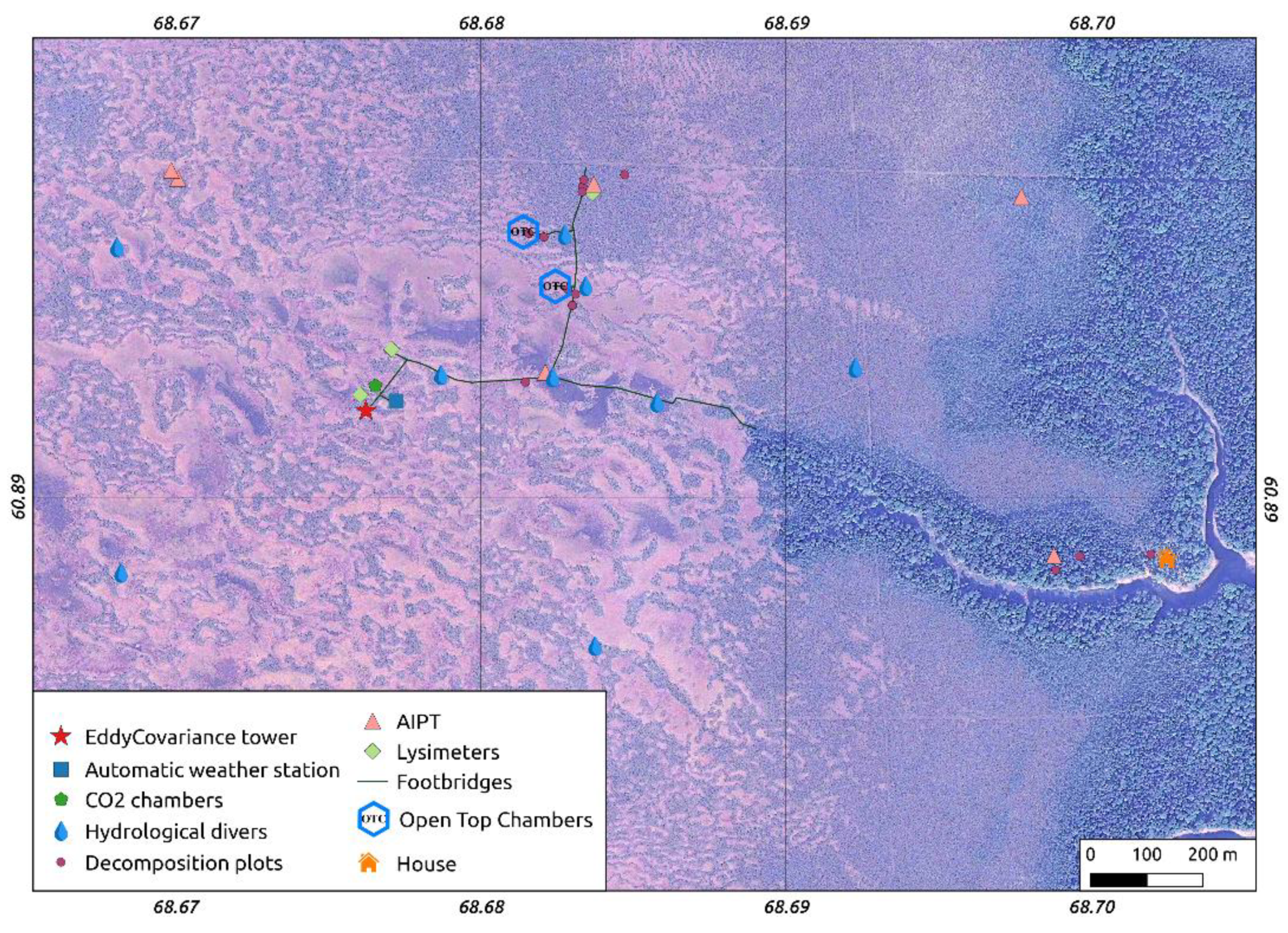
2 fluxes at the ecosystem scale. The estimation of long-term peat accumulation rates provides data on mediated peatland carbon balance. All carbon transformation processes essentially depend on meteorological conditions, energy, and water cycles characterized by high temporal variability. The local observations of meteorological and hydrological parameters were organized using automated weather stations and autonomous water level data loggers. A distributed observation network was constructed to collect data from various peatland landscapes. Annual Sphagnum growth can be used as a complex indicator of the impact of environmental conditions on ecosystem functioning. All information on the Mukhrino FS activities is presented on the official website: www.mukhrinostation.com (accessed on 1 August 2021). The aim of this paper is to summarize the results of peatland carbon balance studies collected over ten years at the Mukhrino FS, to reveal the gaps in the existing monitoring system, and emphasize milestones for the future development of the MFS.

2. Materials and Methods

2.1. MFS Site Location

The MFS is located in the central part of West Siberia in the middle taiga bioclimatic zone, 20 km south-west of Khanty-Mansiysk city, on the second terrace of the left bank of Irtysh River (near the confluence with Ob River). The MFS research area is in the north-east part of the Mukhrino pristine mire complex, which covers a total area ~75 km2 (Figure 1). The extensive area to the south-west is represented by the peatland and lake landscapes of the Kondinskaya lowland, interspersed with forests along the rivers. The MFS area covers ~1 km2 and has a 2 km long system of boardwalks, an energy supply complex (solar panels and wind generator), and permanent hydrometeorological and biodiversity monitoring plots for different elements of peatland ecosystems (microtopes).

2.2. Landscape Position and Vegetation

The Mukhrino mire complex according to [37] is an oligotrophic raised Sphagnum bog. It occupies a local watershed between two small streams, the Mukhrina and Bolshaya rechka, and water discharges to both (see Figure 2). On the eastern side the Mukhrino bog margin is formed by a terrace scarp which rises 2–6 m above the Mukhrina stream valley. The shape of the scarp is undulated by active backward erosion by several source brooks of the Mukhrina stream [38].
Azonal vegetation is represented by the dark coniferous forests and their post-fire stages typical for the middle taiga of Western Siberia. The pine forests are found only on sandy soils of fluvio-glacial deposits (Konda lowland, Surgut Polesie). Forests are limited by well-drained river terraces and flat hills between the vast oligotrophic peatlands that cover the main areas of the watershed territory. In total, peatlands occupy ~50% of the area, with a share of minerotrophic and mesotrophic mires of less than 3% [39]. Azonal vegetation is represented by the meadows and willows in the vast (10–30 km wide) floodplains of the Ob’ and Irtysh rivers, which are flooded 2–4 months a year.
The vegetation cover is commonly patterned, and therefore a three-level hierarchical approach was used for its description. 1: Large land units (5–30 km) recognizable on the regional scale (Figure 1), in the text numbered by Latin numerals. 2: Mid-scale land units (Figure 2A), in the text numbered by Arabic numerals. 3: Small land units (~100 m2), which are relatively homogeneous land units (microtopes) dealt with in the field (Figure 2B), and in the text are highlighted by number and letter (for instance, 1b. Sphagnum lawns).
I.
Ombrotrophic (Sphagnum dominated) raised bogs:
1.
Ridge-hollow-pool patterned bogs and water tracks. This is the most waterlogged peatland complex consisting of three microtopes:
1a.
Dwarf shrubs-Sphagnum ridges with Chamaedaphne calyculata, Andromeda polifolia, Sphagnum angustifolium, S. magellanicum, S. fuscum.
1b.
Sphagnum lawns. Size of the lawns is 1000–10,000 m2 and occupied by Carex limosa, Eriophorum russeolum, Scheuchzeria palustris, Sphagnum balticum, S. papillosum.
1c.
Water pools and waterlogged hollows with Sphagnum majus, S. jensenii, S. lindbergii, Carex limosa, Eriophorum russeolum. Water on the surface and sparse sphagnum cover or slightly higher in the beginning of summer and after long periods of rain.
2.
Ridge-hollow patterned bogs. This mire type is the most widespread ombrotrophic patterned bog complex in West Siberia consisting of pine dwarf shrubs-Sphagnum (ryam) ridges and Sphagnum hollows more or less oriented across a rainwater flow. These complexes are situated usually on very slight sloping areas (gradient 0.003–0.008 m/km). The configuration and spacing of the ridges and hollows are related to the slope gradient of the peatland surface, but mostly they have an equal share in the complex. The ridge microtopes are dryer and 25–50 cm higher than hollows.
2a.
Pine-dwarf shrubs: Sphagnum ridges with Pinus sylvestris, Ledum palustris, Chamaedaphne calyculata, Sphagnum fuscum. The pine height is usually 0.5–2.0 m and 3–10% cover.
2b.
Sphagnum hollows. Vegetation is similar to 1a, but the size of hollows is smaller (10–100 m2).
3.
Dwarf shrub: Sphagnum bog with sparse low pine trees (“Open bog”) with Pinus sylvestris, Chamaedaphne calyculata, Eriophorum vaginatum, Sphagnum angustifolium, S. divinum. The dwarf pine layer is very sparse or absent. These mire types occur on the border between oligotrophic raised bog and mineral uplands. This transition zone usually has a width of 100 to 200 m, rarely wider. They also may be developed in the transition (boundary) zone between raised bogs and minerotrophic fens.
4.
Wooded pine-dwarf shrub-Sphagnum bog (ryam)
4a.
Typical ryam with Pinus sylvestris, Ledum palustris, Chamaedaphne calyculata, Sphagnum fuscum. Ombrotrophic dwarf shrubs: Sphagnum hummock peatlands wooded by pine trees 0.5–4 m high. This type of bog is very common in West Siberia and covers large homogeneous areas or is presented as ridges in patterned bog complexes.
4b.
Tall ryam with Pinus sylvestris, Ledum palustris, Chamaedaphne calyculata, Vaccinium myrtillus, Sphagnum angustifolium, S. divinum. Differs from the typical ryam by the height of the tree layer (6–10 m) and dominated by Sphagnum species in the ground layer.
4c.
Ryam with small cotton grass: Sphagnum hollows with Pinus sylvestris, Ledum palustris, Chamaedaphne calyculata, Sphagnum fuscum on ryam hummocks and Eriophorum vaginatum, S. balticum in hollows. Differs from typical ryam with a presence of small hollows covered by cotton grass-Sphagnum balticum communities.
II.
Mesoologotrophic fens:
5.
Sedge-Sphagnum fen (incl. sparse low birch fens) with Betula pubescens, Carex rostrata, Oxycoccus palustris, Sphagnum angustifolium, S. fallax, S. flexuosum). The tall sedge Sphagnum through-flow fens fed both by rain run-off and groundwater are often sparsely wooded by small birch trees.
III.
Upland forests
6.
Dark coniferous and mixed forest with Pinus sibirica, Abies sibirica, Picea obovata, Populus tremula, Betula puescens and Vaccinium myrtillus, Maianthemum bifolium, Linnaea borealis, Gymnocarpium dryopteris, Hylocomium splendens, Pleurozium schreberi in the ground layer. There are typical climax forest communities on loamy soils in the West Siberian middle taiga.
7.
Small-leaved forest with Betula pubescens, Populus tremula in the upper layer, young Pinus sibirica, Abies sibirica, Picea obovata trees, and Vaccinium myrtillus, Pleurozium schreberi on the ground. These are different stages of the post-fire succession.
IV.
Floodplains
8.
Floodplain willow (Salix triandra, S. alba, S. viminalis, S. dasyclados). Highest floodplain level, flooding frequency 25–50%.
9.
Meadows with Phalaroides arundinacea. Mid floodplain level flooded for 1–2 month, flooding frequency 50–75%.
10.
Sedge wetlands with Carex aquatilis, Carex juncella. Low floodplain level flooded every year for 2–4 month.
Photos of the peatland landscapes available online at [40].

2.3. Field Data Collection and Analysis

2.3.1. Meteorology

Hydrometeorological data are available for the MFS from 2010 to 2019 for two sites located at two distinct microtopes [41]. Data on air temperature, air humidity, atmospheric pressure, wind speed and direction, incoming and outgoing shortwave radiation, net radiation, and soil heat flux were recorded at three automated weather stations (In Situ Instruments AB, Sweden. Table A1 in Appendix A). Two stations were located at a small pine-dwarf-shrub-Sphagnum ridge (vegetation type 2a) and one station at a Sphagnum hollow (evgetation type 2b) (see automatic weather station location at Figure 3). The hollows represent lower-lying parts of the microtope with the water level near the surface (0–15 cm below the surface), while the ridges are elevated dry microsites with the water level at a 20–40 cm depth (see Section ‘Hydrology’ for more information). The weather stations recorded data at 15 min intervals in 2010–2011, at hourly intervals in 2012–2013, and half-hourly intervals since 2014.
All data are available via the open-source DEMIS-SDR (Dynamic Ecological Information Management System—Site and dataset registry) web portal [42] and Zenodo [43].

2.3.2. Hydrology

For monitoring of the peatland’s water table dynamics, a network of 11 piezometers was established (see Figure 3) at representative locations of the main microtopes occurring in the Mukhrino bog (see section on Peatland landscape structure).
A pressure-logger (Mini-Diver D1501, accuracy ±5 mm of water, frequency measurement 30–180 min) was installed in groundwater observation tubes (5 cm diameter) with a filter at 100–250 cm below the peat surface. The groundwater wells were fixed in the mineral soil (at a depth of 350–550 cm below the peat surface, depending on the location) to have a fixed reference datum and avoid vertical changes of position due to peat volume expansion or compression [44]. For barometric compensation, the air pressure was recorded with a pressure-sensor (Baro-diver, accuracy ±5 mm of water, frequency measurement 30–180 min) placed in the center of the mire 2 m above the surface. The first measurements started in 2008 [45] and were used to develop and validate steady-state and dynamic groundwater models [38].
To estimate actual evapotranspiration, a network of lysimeters was installed in 2015. Four standard open top containers (Russian traditional hydrometeorological equipment GGI-3000) with pressure-loggers (Mini-Diver D1501) were installed in the main microtopes: open water, hollow, ridge, and ryam. The containers were filled up with local litter and representative living vegetation layers to simulate real (actual) evapotranspiration, which was calculated from fluctuations of water level and precipitation.
The amount of snow water for the main microtopes has been measured manually at the end of March since 2010. A metal tube (12 cm diameter) was used to cut an exact volume (for whole snowpack depth) of snow. Snow depth was measured by a pole snow gauge, and the volume of water stored in bulk snow was measured by the weighting method.
Rainfall was measured with a rain gauge (HOBO RG3, resolution 0.2 mm, “by event” data logging) installed in the ryam and ridge microtopes.

2.3.3. Chamber Measurements of Carbon Dioxide Fluxes

The automated monitoring of carbon dioxide fluxes at ridge-hollow patterned bog was performed from 2017–2019 using a portable atmospheric soil measuring system (ASMS) with two transparent chambers (Figure A1 in Appendix A). Automated chambers were placed at a pine-dwarf shrubs Sphagnum ridge (vegetation type 2a) and Sphagnum hollow (vegetation type 2b). The ASMS can measure and record simultaneously the following environmental characteristics: air temperature (Ta) and humidity (RH) (at height of 2 m above the ground and at the ground surface), PAR (photosynthetic active radiation; incoming solar radiation in the 400–700 nm spectral range), carbon dioxide content, and water vapor pressure in the air samples. The system includes a two-channel gas analyzer Li-7000 (Li-COR Biogeosciences, Lincoln, NE, USA) and two measuring chambers with a volume of 120 L. The chambers are closed for five minutes every hour (or three hours in 2017) to provide a flux measurement. The rest of the time they remain open. The air for a sample is continuously pumped through the chamber and the gas analyzer during the observation period using a diaphragm pump 7006ZVR (Gardner Denver Thomas GmbH, Germany, Fürstenfeldbruck) with a flow rate ~2 L/min. The measurements of the concentrations of CO2 and H2O, Ta, RH, and PAR are continuously stored in the ASMS and transferred to a web server.
The automated system operated in a measuring mode from July to August in 2017, and from May to October in 2018 and 2019. The CO2 flux was calculated using a specialized software module developed in the Matlab R2014b (MathWorks, Natick, MA, USA) using a linear model for changing the concentrations in the chambers during the first two minutes of data sampling. To obtain continuous data records, to extrapolate them to other periods when experimental data are missing, and to calculate the annual carbon budget of the ecosystem, a model of total ecosystem carbon exchange was used [46]. The measured total NEE was partitioned into gross primary production (GPP) and total ecosystem respiration (ER) components. The model was calibrated using all available data sets on carbon dioxide fluxes in 2017–2019 [47] and extrapolated for the period 2010–2016.

2.3.4. Eddy-Covariance Measurements

An eddy-covariance (EC) tower was deployed in a representative part of the Mukhrino bog at ridge-hollow patterned bogs in 2015 to provide continuous, ecosystem-scale data on GHG exchange and energy balance [48]. At the time of establishment, it was the first permanent EC setup within a radius of ca. 1000 km and the only one in Western Siberia. The EC instrumentation consisted of a CO2, H2O analyzer (LI-7500) and a 3D ultrasonic anemometer (Gill R3, Gill Instruments, Lymington, UK). During the first season, the measurements were made from May to August 2015 and provided appropriate flux data coverage for the entire growing season. Raw EC data were processed using EddyUH software v.1.7 [49] according to state-of-the-art methodologies [50]. An energy balance closure of 0.99 was observed, pointing to the good quality of the EC data. The 4 m a.g.l. EC sensor mounting height resulted in a 70% footprint zone with a radius of ca. 89–202 m depending on atmospheric stability, covering a representative mix of ridge and hollow microsites (Figure A2 in Appendix A).

2.3.5. Sphagnum Annual Growth and Production

Measurements of Sphagnum annual growth were started at the Mukhrino FS in 2013 as part of the total ecosystem primary production estimate [51]. A total of 57 plots were located along the boardwalks of the research area in the main types of ombrotrophic bog. Measurements were carried out using the cranked wire approach (its modified brush-wire version) for up-growing species (Sphagnum fuscum, S. divinum, S. angustifolium, S. papillosum, S. capillifolium), or individual wire rings for side-growing species (S. majus, S. jensenii, S. balticum) (see Table A2 in Appendix A). Part of the plots were located under warming experiment conditions (Open Top Chambers, OTC) to study the influence of raised temperatures on growing rate [52]. Each species was studied in two to six plots (depending on species frequency) in several locations within ~700 m radius to cover spatial variations. Each plot contained ten replicate markings (brush-wires or individual rings) to cover individual variability or the occasional loss of the markings.
The markings were installed in November to start measurements from May until November of the following year. The measurements were done using a ruler (accuracy 0.5 cm) and inserted in the table formatted by the Darwin Core standard for biological diversity data, which available openly in GBIF [53].

2.3.6. Decomposition Rate of Native and Standardized Substrates

To estimate the conditions of organic matter decomposition dynamics in different ecosystem types at the Mukhrino FS, a series of experiments was launched in 2016. Occasional studies on the decomposition of peat and Sphagnum spp. were performed earlier by [51,54]. The classical approach of litter bags was used to estimate weight loss, including standard litter type (tea) and native litters (see Table A3 in Appendix A) under both natural and experimental warming conditions (Open Top Chambers). The standard tea substrate was used to compare habitat effects and supplement the data to global projects on decomposition dynamics [55,56,57].
The decomposition of native litters was studied in three plots (two replicas of four bags with a particular litter type), located in the major ecosystem types: wooded pine-dwarf-shrubs-Sphagnum bog (ryam), Sphagnum bog (lawn), and coniferous forest. To study the long-term dynamics of litter decomposition, a series of bags were located for one, two, three and four years (and one series for ten years of decomposition). The series of bags for 1–4 years of decomposition had been installed each year since 2016. To supplement the variety of ecosystems, another three plots were set up in the deciduous forests ten years and 40 years after a clear-cut, and in the nearby old-growth coniferous forest. To study interannual dynamics, a new series of bags for 1–4 years of decomposition had been prepared each autumn since 2016 (a total of five installations were made by 2021) and will be continued in the future.
The tea was weighted and buried in the beginning of the vegetation season (end of May). The extraction was done after three months (beginning of September). One series of long-term decomposition dynamics of standard tea (three months, one, two, three, four years) was installed once in 2016. Since 2017, the tea has been buried only for a short decomposition period (three months) (see Table A3 in Appendix A).
The decomposition experiment of native litters was done according to [57]. The leaves of native plants were collected in autumn, dried, and sewed into nylon bags measuring 10 × 10 cm (mesh size about 0.2 mm), labeled, and buried in the upper 0–5 cm of the soil horizon.
After an incubation period, the litter bags were excavated, cleaned from the attached soil and roots, and dried. The weight measurements were compiled in the table formatted by the Darwin Core standard for biological diversity data, which is available openly in GBIF [58].

2.3.7. Peat Sampling and Lab Work

The peat cores (35 in total) were extracted at the main microtopes of the Mukhrino bog to cover a spatial heterogeneity. A Russian corer (50 cm length, 5 cm in diameter) was used for peat extraction. The cores were described in the field, wrapped in plastic film, packed into cases, and stored at 4 °C.
Carbon (C) content was determined by an elemental analyzer (EA-3000, EuroVector, Italy, Pavia) using a thermal conductivity detector and Atropine standard (C = 70.56%, N = 4.84%, H = 8.01%, O = 16.59%). The rates of peat and carbon accumulation were calculated by dividing the peat depth or amount of accumulated carbon per unit area by the time of its formation, according to [59].
Plant macrofossils were identified under a binocular microscope at 910–40 magnification (Zeiss Axiostar, Oberkochen, Germany) using our own reference collection. Relative abundances (%) of plant macrofossils and their total diversity were used to describe peat composition and to determine the peat type.

2.3.8. Mapping

All maps were prepared by Open software QGIS [60] and GRASS [61]. A supervised classification (smap method [62], with the number of teaching polygons not less than 30 per landunit) was applied to the satellite images from Landsat-8 (set to 100 m resolution median values from May until August for the period 2017–2020) and MODIS (median values from May until August for the period 2017–2020) resources which were prepared via the Google Earth Engine portal.

3. Results

3.1. Meteorology

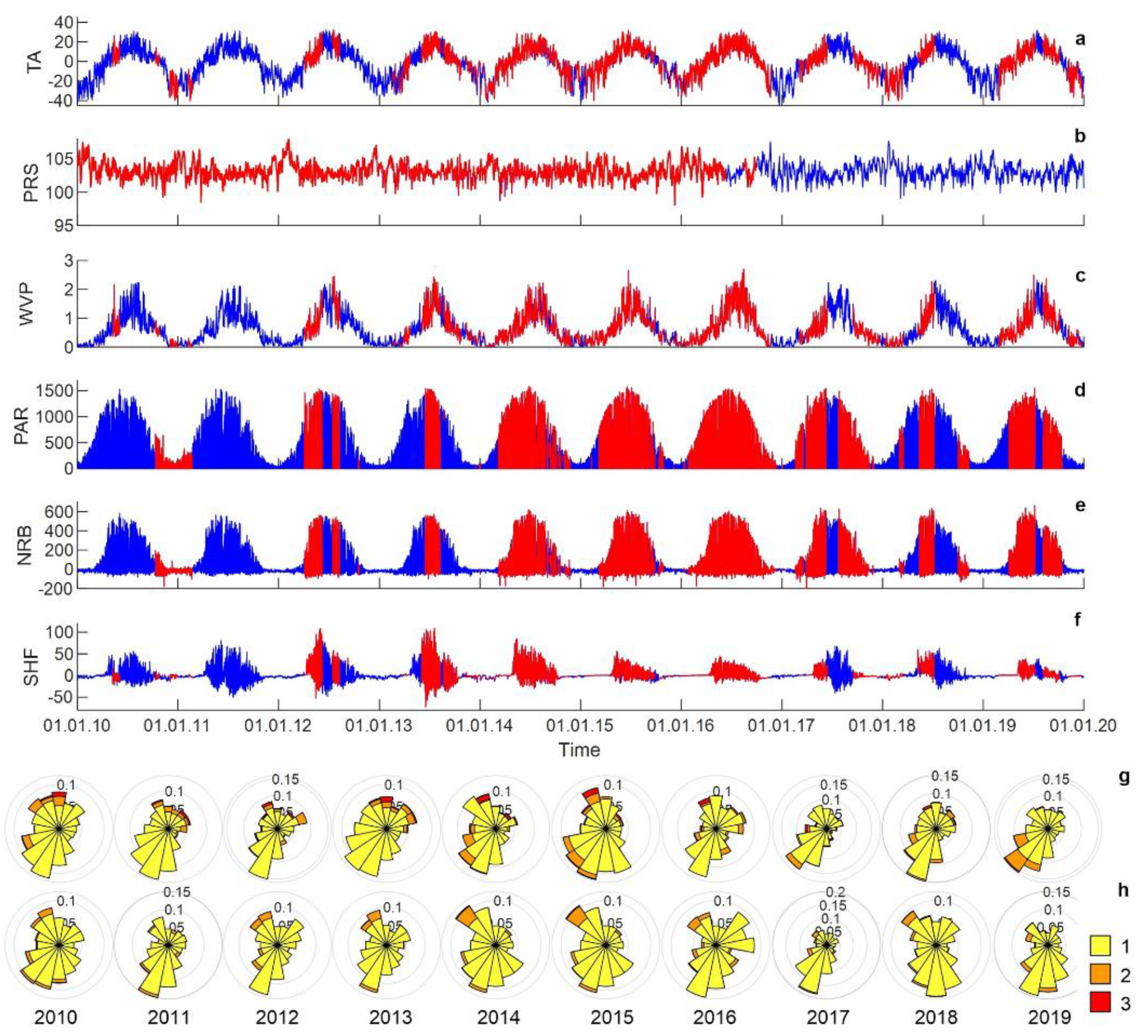
Annual, seasonal and diurnal variations of the hydrometeorological parameters were observed at the MFS (Figure 4). The monthly air temperature varied from 13.8 to 17.4 °C in July and from −27.8 to −17.3 °C in January, whereas the absolute temperature minimum was −45.0 °C at 22:00 on 21 December 2016, and the absolute temperature maximum was 32.9 °C at 16:00 on 5 August 2016. For the period from 2010 to 2019, the average mean annual air temperature at the site was −1.0 °C, with the mean monthly temperature of the warmest month (July) recorded as 17.4 °C and for the coldest month (January) as −21.5 °C.
The air humidity in winter was much lower than in summer. The monthly water vapor pressure varied from 0.05 to 0.16 kPa in January and from 1.22 to 1.69 in July. The differences between measurements of air parameters obtained at the ridge and the hollow sites were insignificant. The two sites are closely situated, and intense air mixing equalizes the air conditions.
The incoming photosynthetically active radiation (PAR) registered at both sites has a maximum at noon, and the value of the maximum rises from December to July. The amount of reflected PAR is closely related to the state of the surface. The albedo for the PAR range (the ratio of reflected and incoming PAR) in summer was about 0.03 and 0.06 at the hollow and ridge sites, respectively. The albedo in winter at snow-covered surfaces was about 0.95 at the hollow site and 0.8 at the ridge site, where small dark branches of trees were present.
The net radiation balance had close maximal values at both sites, but the diurnal course of net radiation at the ridge was shifted one hour later compared with the hollow site. The January net radiation was negative and varied within a range from −8 to −18 W m-2 during a day. The daily averaged soil heat flux was negative from October to March. The maximal heat flux into the soil was observed in June at approximately 18:00 local time. The amplitude of diurnal variations of soil heat flux at the hollow was two to three times higher than at the ridge. The soil heat flux sensors at the ridge were located under a porous mat of weakly decomposed dead mosses isolating the peat layers from heating.
Maximum snow storage was recorded on 18 March 2013 when the snow depth reached 95 cm on the ridge site. The winter of 2010–2011 was the season with the weakest snowpack. The snow cover at the end of winter on 16 February 2011 was only 64 cm. Complete melting of the snow took place between 16 April and 19 May depending on the year. The average duration of the snow cover period was 191 days. South-south-east winds prevail at the observation site, but winds with speeds above 5 m s−1 were mostly of a north-east origin. The median wind speed value at 10 m was 1.8 m s−1, while at 2 m above the surface it was only 1.0 m s−1. The wind rose structure was similar for all observation years, except 2017 and 2019.
The meteorological data presented and described is available for download from [42,43]. Gap-filled, quality controlled, and raw observation data are provided separately.

3.2. Hydrology

Water saturation of the peat is one of the leading factors of GHG balance in peatland ecosystems. Favorable conditions for overwatering of soils were formed in the taiga of Western Siberia. Positive water balance is formed due to predominance of precipitation over evaporation by more than 1.5 times. Such wetting conditions have existed in the taiga of Western Siberia for about 10,000 years. However, the annual water balance in the peatland can vary, and in some years it has even been negative (for example, 2010 and 2020).
The Mukhrino bog is fed only by rain and snowmelt water. The average annual amount of precipitation is 470 ± 68 mm, where ¼ is snow (~126 mm). Most of the snow is accumulated by ryams and ridges, with snow depths of ~61 cm and ~67 cm (~139 mm and ~131 mm of precipitation), respectively. Hollows accumulate a thinner snowpack with depths of ~38 cm (90 mm of precipitation).
The highest water level coincides with the melting of snow at the end of April to the beginning of May. Upper peat layers (up to 50 cm depth) are usually frozen during the snowmelt period so that the produced snowmelt water cannot infiltrate into the peat and is also blocked by the frozen ridges; therefore, ponds are formed in the hollows. As soon as the ridges are defrosted the water flows superficially over and through the acrotelm (overland flow) to the streams [38]. When the upper peat layer melts down, a part of the ponded water rapidly percolates downward into the peat layers causing a dramatic increase of the water level. During the summer period the WTE is lowered gradually by the evapotranspiration surplus over precipitation [
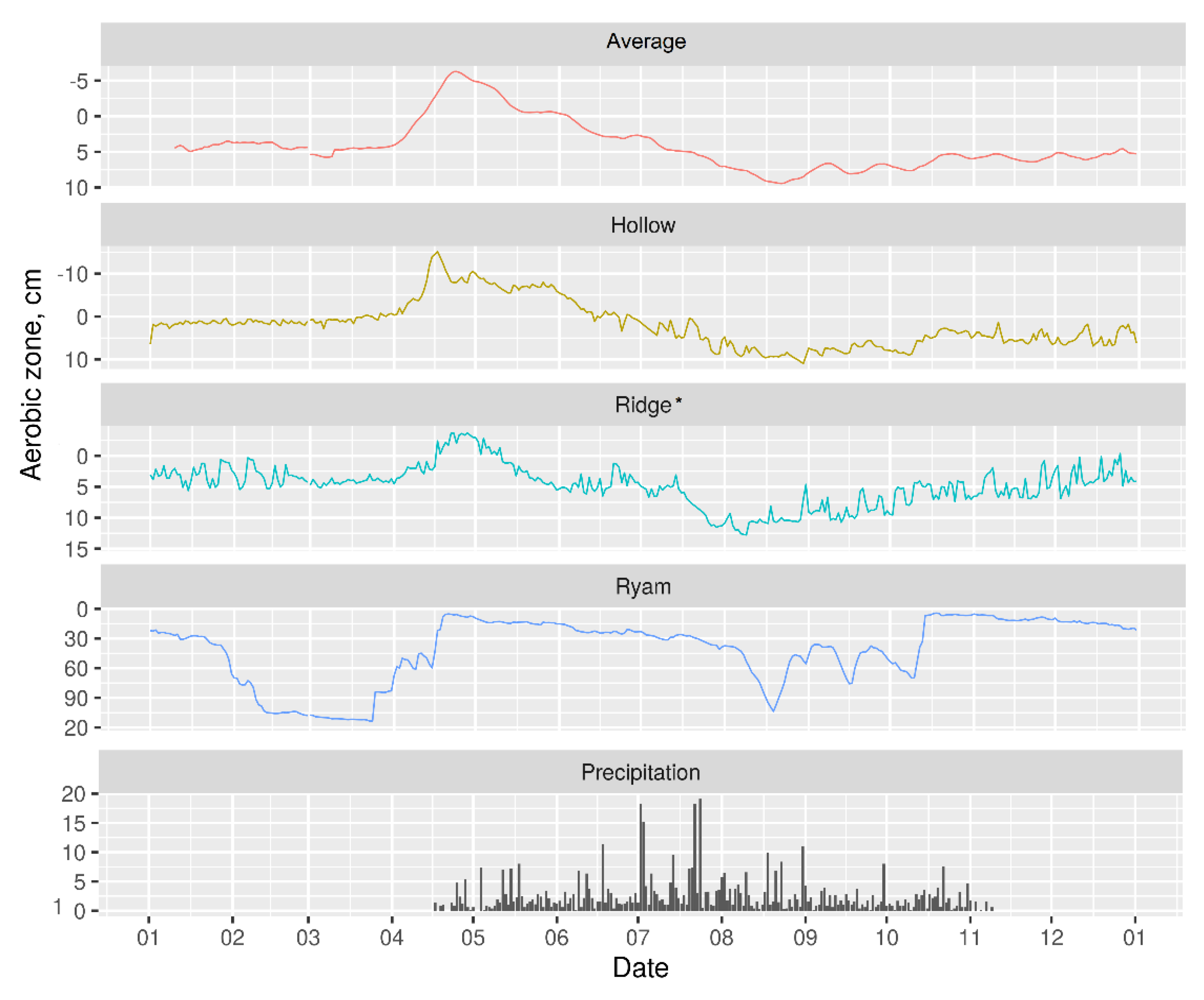
49]. The lowest water level is recorded at the end of summertime (usually in August); however, the WTE rose temporarily after intense rain events in summer or autumn. In autumn, such a temporal rise was more prominent while the evapotranspiration decreased with the lowering of air temperatures (see plot “Average” in Figure 5). Discharge from the streams stopped in mid-October when the water froze.
The occurrence of superficial water flows was proved with the hydrological model [38], not only during the period of existence of frozen peat layers but also during the summer, and in particular after rain events. The low hydraulic conductivity of the peat layers limits infiltration and favors overland flow. It appeared from the modelling that more than 90% of the water was discharged superficially across the acrotelm mostly through hollows.
WTE change is dependent on the microtope (Figure 5). It is small in the center of the bog and high at its edges. The smallest fluctuations were found at the hollows, where water rose to 15 cm above the surface in April and dropped to 10 cm below the surface in September (average WTD is ~2 cm). The ridges had wider WTD movement, rising to 4 cm above the surface in April and falling to 14 cm below the surface in September (average value was 5 cm).. A piezometer on the ridge was installed in a local depression ~25 cm deep, i.e., the actual WTD was ~30 cm below the peatland surface. The water table can rise into the acrotelm at ridges, which in the lower part have a lower effective porosity. After rain the WTD may rise a little above the water level in the adjacent hollow but falls down a few cm below the hollow through evapotranspiration.
The highest WTD amplitude was found for the well-drained ryam, where in early spring when the water rose close to the peatland surface (4 cm below) and dropped to ~120 cm below surface (some years even 190 cm below the surface) at the beginning of autumn (the average value was 41 cm).
Near the margin of the bog, close to the terrace scarp, the upper peat layers are drained. As a result, the peat settles, and cracks are formed. During rain events the cracks were filled up with water, which resulted in a relatively high rise of the WTE as measured in the peat. After rain, the WTE was lowered deeply by vertical percolation and evapotranspiration.
Because the peat soil is fully water-saturated, precipitation events result in a WTE rise comparable to the precipitation intensity. An amount of 10 mm precipitation results in a maximum rise of about 1 cm, but less in summer when part is evaporated, and another part is lost by lateral run off.
The evapotranspiration values for different microtopes are presented in Table 1.
The WTD cannot be easily measured everywhere and at all times. Water levels have been recorded in filter tubes at some depths below the surface. In particular, the water levels in hollows cannot be directly converted to water levels below the moss surface. If precipitation or snow melt water is supplied, the floating root mat (quak mire) will partially move upwards, and a measured groundwater level rise is not seen as a change in WTD. In the case of very intensive water supply, the root mat cannot follow completely and ponding results. Conversely, during a dry period, due to evapotranspiration, the root mat lowers and the environmental conditions for the vegetation (and therefore the carbon gases exchange with the atmosphere) remain almost the same. This process of root mat rise and fall may be subject to hysteresis.

3.3. Carbon Dioxide Fluxes at a Local Scale

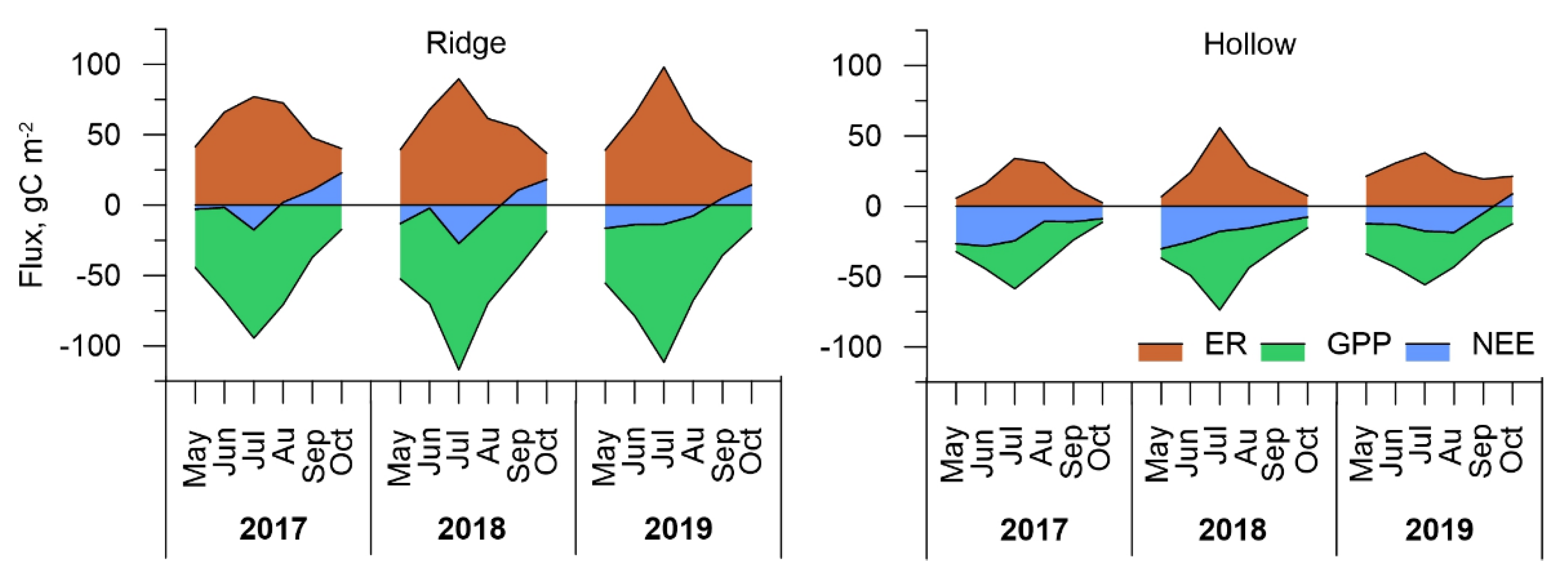
Time series of gap-filled modeled ER, GPP, and NEE fluxes were integrated for each month of the study period. The annual variability of monthly carbon fluxes for ridge and hollow sites is shown in Figure 6. The largest ER efflux was obtained in July 2019 at the ridge site (98.1 gC m−2). Respiration rate at the hollow site reached maximum values in July 2018, and were somewhat lower than at the ridge site (55.8 gC m−2). In May, the total respiration did not exceed 21.4 gC m−2 at the hollows and 41.5 gC m−2 at the ridge sites. The most intense emission was obtained for the ridge site where various vascular species strongly contribute to the autotrophic part of respiration and a thicker acrotelm layer promotes the aerobic decomposition of plant residuals. The ER rate in September and October was still high at the ridge site, but because of low GPP the ridge acted as a source of CO2 for the atmosphere.
The photosynthetic activity of bog vegetation began in early spring, and the GPP rate reached rather high values in May at 37 and −55.5 gC m−2 for hollow and ridge sites, respectively. GPP reached its maximum rates in July with −117 gC m−2 at the ridge site and −73.7 gC m−2 at the hollow site. June and August were characterized by lower values of GPP because of lower PAR values.
The largest variations of carbon flux were observed at the ridge site, where seasonal maximums in absolute values of ER and GPP significantly exceeded the corresponding values at the hollow site. The hollow site had smoother flux dynamics and lower absolute values of ER and GPP. Despite the differences in GPP and ER between both sites, monthly NEE was higher at the hollow site. The summer month rates of NEE are presented in Table 2. The maximal carbon uptake occurred in July at both sites. Positive NEE values (up to 22.9 gC m−2) were obtained for September–October at the ridge site.
The growing season (May–October) cumulative NEE, calculated by integrating the monthly averaged diurnal NEE rates at the hollow site was−110, −107.8, and −57.8 gC m−2 in 2017, 2018, and 2019, respectively. Our results show that the amount of CO2 captured from the atmosphere at the ridge site was lower, resulting in −22 and −32.1 gC m−2 in 2018 and 2019. A net CO2 emission of 13.4 gC m−2 was observed at the ridge site in 2017.
The results of field measurements of CO2 fluxes at the ridge-hollow complex in combination with the suggested mathematical model allowed us to adequately estimate the NEE, ER, and GPP rates for ridge and hollow sites at an oligotrophic bog in the middle taiga zone of West Siberia. The cumulative CO2 uptake rates exceeded cumulative respiration rates at both experimental sites. The three-year average growing season NEE at the hollow site was significantly higher (−91.9 gC m−2) than at the ridge site (−13.6 gC m−2). GPP and ER rates at the ridge site were higher than at the hollow site.

3.4. Carbon Dioxide Fluxes at Ecosystem Scale

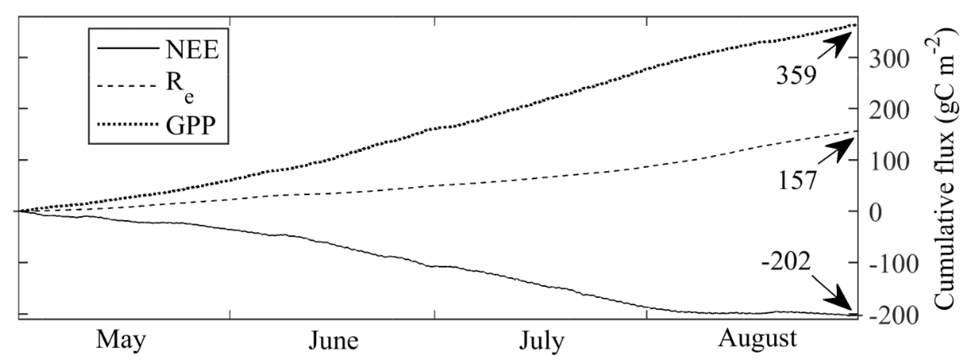
The cumulative May-August NEE was −202 gC m−2 in 2015, with the monthly cumulative values being −35, −72, −79, and −16 gC m−2 month−1 for May-August, respectively. The May-August cumulative NEE of −202 gC m−2 splits into Re = 157 g C m−2 and GPP = 359 g C m−2 (Figure 7). High net C uptake was likely driven by an early, warm, and wet spring, which allowed for the early development of aboveground biomass. Although several cold fronts later in the summer almost completely stopped GPP for short periods, they did little to affect the steady seasonal course of C uptake. This ecophysiological stability is corroborated by the Bowen ratio, which very gradually reduced from 0.32 in May to 0.26 in August (for further details on the study, see [48]).
EC measurements using the same setup were continued in 2016. Drier, hotter conditions in that year resulted in a much lower cumulative May-August NEE than in 2015 (paper in preparation). In 2019, the EC setup was expanded with a CH4 analyzer (Li-Cor LI-7700); CH4 fluxes similar to those of other boreal mire ecosystems were observed (paper in preparation).

3.5. Sphagnum Annual Growth and Production

A total of 832 measurements of annual Sphagnum growth increments were performed during two years of monitoring. About a half of the measurements (338) of Sphagnum balticum annual growth were installed in plots under experimental warming (OTC) and used to study the effect of climate warming on primary production.
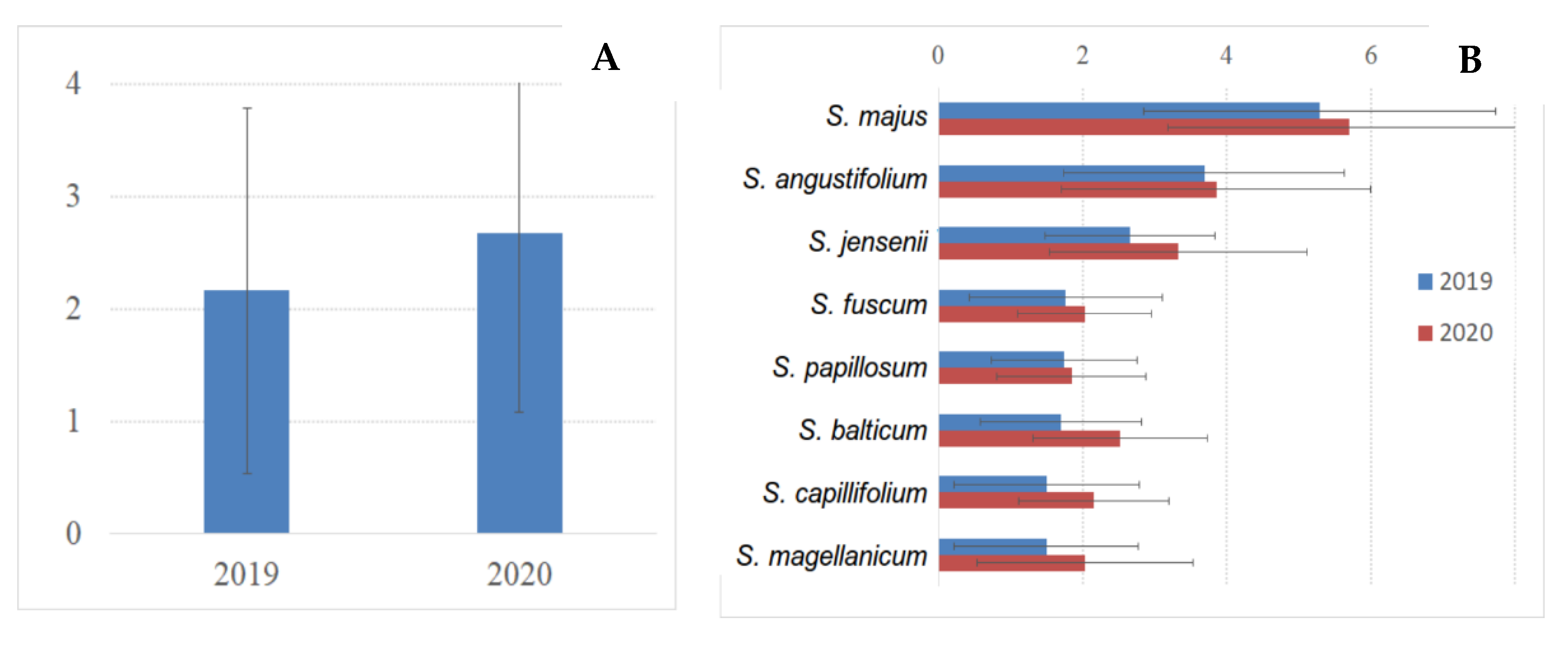
The mean annual growth increment differed between the studied species from 1.5 to 3.6 cm per vegetation season (Figure 8). Five up-growing species had the lowest annual growth rate and did not differ significantly between each other (Sphagnum divinum, S. capillifolium, S. balticum, S. papillosum, S. fuscum). Three side-growing species (Sphagnum jensenii, S. angustifolium, S. majus) showed a higher annual growth rate and varied significantly between each other.
Two subsequent years of measurements showed differences in annual growth rate (Figure 8). The values were significantly higher in 2020 compared to 2019 for almost all species. The climate conditions influencing the annual dynamics will be studied in more detail after the accumulation of data for several years.
The study of Open Top Chambers showed no significant effect of temperature rise on Sphagnum balticum growth rate in both vegetation types (Eriophorum-Sphagnum bog and graminoid-Sphagnum bog). This might be explained by the insignificance of a slightly increased temperature impact on the primary production of Sphagnum as opposed to other factors (species-specific physiology, precipitation, or ground-water level).

3.6. Decomposition Rate of Native and Standardized Substrates

Around 1500 litter bags had been extracted by the spring 2021 (see Table A4 in 
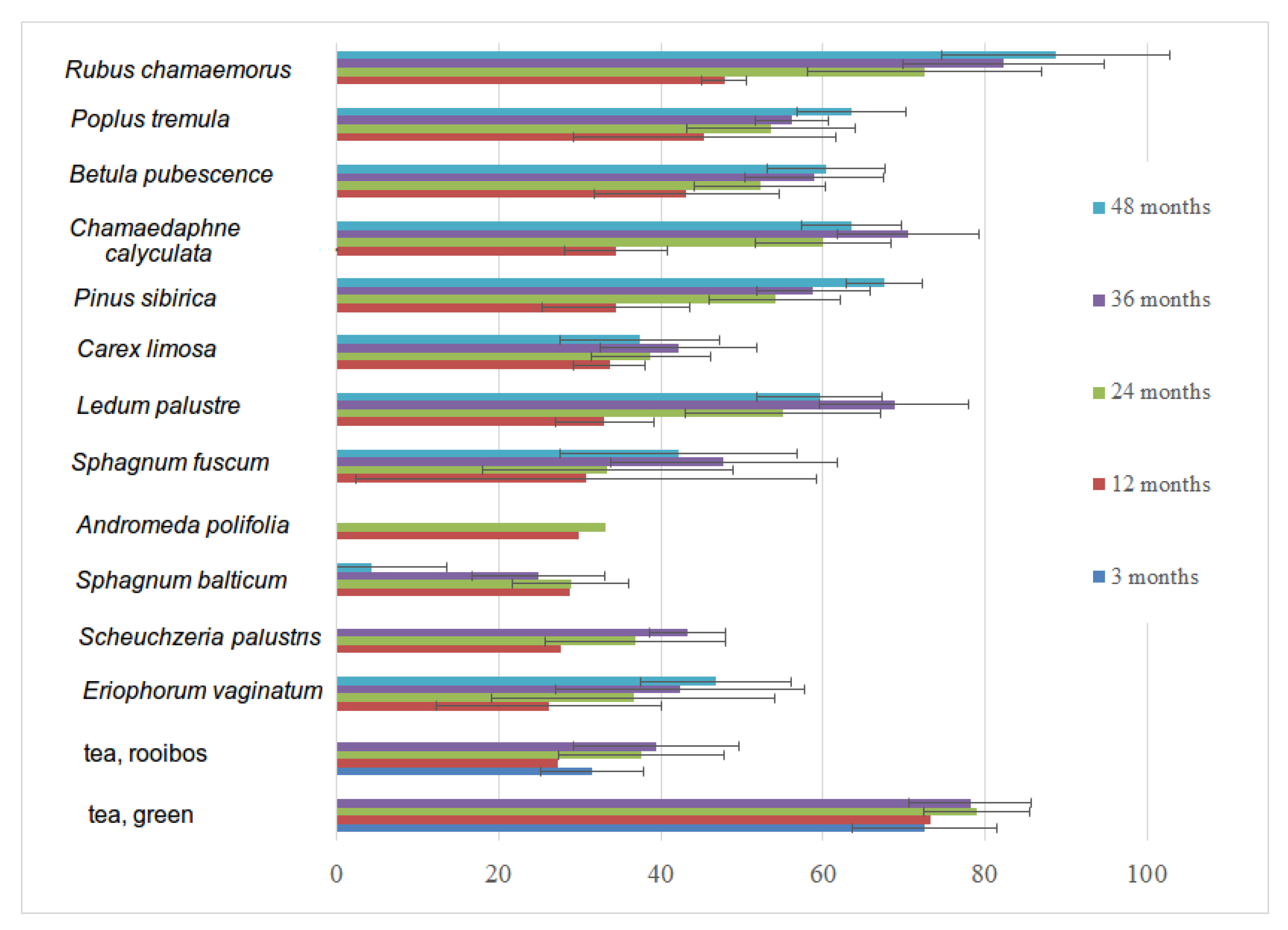
Appendix A). The native litter types have one series of a four-year decomposition period (eight bags per type), two series of three years (16 bags), three series of two years (24 bags), and four series of annual decomposition period (32 bags). The standard tea had one full series of long-term decomposition (1, 2, 3 and 4 years) and four series for decomposition for three months.
The most resistant substrates (minimal weight loss after one year of decomposition) were Eriophorum vaginatum, Scheuchzeria palustris, Sphagnum balticum, Andromeda polifolia, and Sphagnum fuscum. The fastest decomposition was observed in Rubus chamaemorus and forest leaves (Figure 9). Only five litter types continued to lose mass after four years of decomposition, nine litter types continued mass loss after three years, and all types continued decomposition during the second year. On average, 83% of the total mass loss between all litter types occurred during the first two years of decomposition. About 93% of the weight loss of green tea occurred during the first year of decomposition, and 7% during the second. The weight of rooibos showed a less abrupt loss, corresponding to 49, 36, and 15% loss during the first three years of decomposition.
There was no significant difference (Wilcoxon rank sum test) between the mass lost in different forest types (old-growth coniferous forest and its deciduous stages after clear-cutting). A significant difference was, however, shown between the forests (all types), treed bogs, and lawns (see Table A4 in Appendix A for more details).
Interannual variations (influence of year-specific weather conditions on decomposition) were studied on one-year decomposition series for native litters and three-month series for tea (four series of bags from 2016 to 2019). The differences were significant (Wilcoxon rank sum test) in interannual variation for several substrates: Rubus chamaemorus, Populus tremula, Carex limosa, Sphagnum balticum, and rooibos tea. This might be caused rather by local installation differences rather than being related to year-specific weather conditions. There were no significant differences (Wilcoxon rank sum test) between the plots with OTC and control plots both for green and rooibos teas.

3.7. Peat Stratigraphy and Rates of Peat and Carbon Accumulation

The Mukhrino bog was initiated as a minerotrophic fen in the Preboreal stage (9360 cal.yr.BP) but older layers of gyttja (10,052.5 cal.yr.BP) and reed peat (10,989 cal.yr.BP) were found in depressions of lakes and ancient riverbeds. Dominant remains of trees (birch, pine, fir), herbs (Menyanthes, Thelypteris palustris, Equisetum fluviatile) and tussock-forming sedges (Carex juncella, C. cespitosa) were found at the bottom layer (average thickness 0.65 m) for the whole area of the peatland. The transitional/mesotrophic peat (~0.5 m) overlays the minerotrophic peat layer and consists of the Scheuchzeria palustris, sedges, dwarf shrubs, and Sphagnum moss remains. The upper part of the peatland (about ⅔) is formed by oligotrophic peat and consists of Sphagnum with interlayers of thin cotton-grass- or sedge-Scheuchzeria-Sphagnum remains [4]. The average peatland depth is 310 cm with local depressions down to 530 cm depths and shallow peat deposits at the peatland edge.
The most frequent peat types are Sphagnum fuscum-peat (share in the peat deposit 22.5%), Sphagnum hollow peat (S. balticum, S. papillosum (12.0%), and Sphagnum oligotrophic peat (S. fuscum, S. angustifolium, S. divinum, S. papillosum, S. balticum (5.7%) [4].
The calculated average peat accumulation rate was 0.075 cm yr−1 (ranging between the different cores in 0.013–0.332 cm yr−1). The maximal rates were found for the upper oligotrophic (0.33 cm yr−1, 50–0 cm, 800 cal. year BP-till now) and bottom minerotrophic (0.28 cm yr−1, 520–360 cm, 10,900–10,000 cal. year BP) layers with the rate dropping to 0.013 cm yr−1 in between.
The carbon accumulation rate was 38.8 gC m−2 yr−1 (ranging in 28.5 and 57.2 gC m−2 yr−1 between the cores). It was evenly distributed over the depth with local peaks (up to 176.2 gC m−2 yr−1) at the different depths.

4. Discussion

An investigation of carbon exchange processes is required to better understand the links between terrestrial ecosystems and both the regional and global climate systems. The peatland carbon cycle represents a component of the global carbon budget with a continuous sink of carbon from the atmosphere [63]. An imbalance between plant uptake of atmospheric CO2 by photosynthesis and the release of CO2 to the atmosphere through ecosystem respiration (the emission of CO2 from vegetation—autotrophic and soil—heterotrophic respiration) results in peat (plant remains) accumulation [64]. A knowledge of the response of GHG fluxes between ecosystems and the atmosphere to climatic variability is crucial for the prediction of future atmospheric levels of GHG [65]. Eddy-covariance and chamber methods are the most widespread in the study of GHG fluxes.
The EC approach is an established and robust technique to quantify turbulent exchanges of scalars such as trace gases, momentum, and energy, between the Earth’s surface and the atmosphere [66]. Chamber measurements have been the prevailing technique to monitor the CO2 exchange between the atmosphere and soil, plant organs, or complete ecosystems [67].
The tower-based EC technique provides continuous observations of carbon, water, and heat fluxes integrated at the ecosystem scale. These multiple years observation results in a variety of sites and biomes in different climatic zones are a critical tool for the quantification of global and regional GHG dynamics [
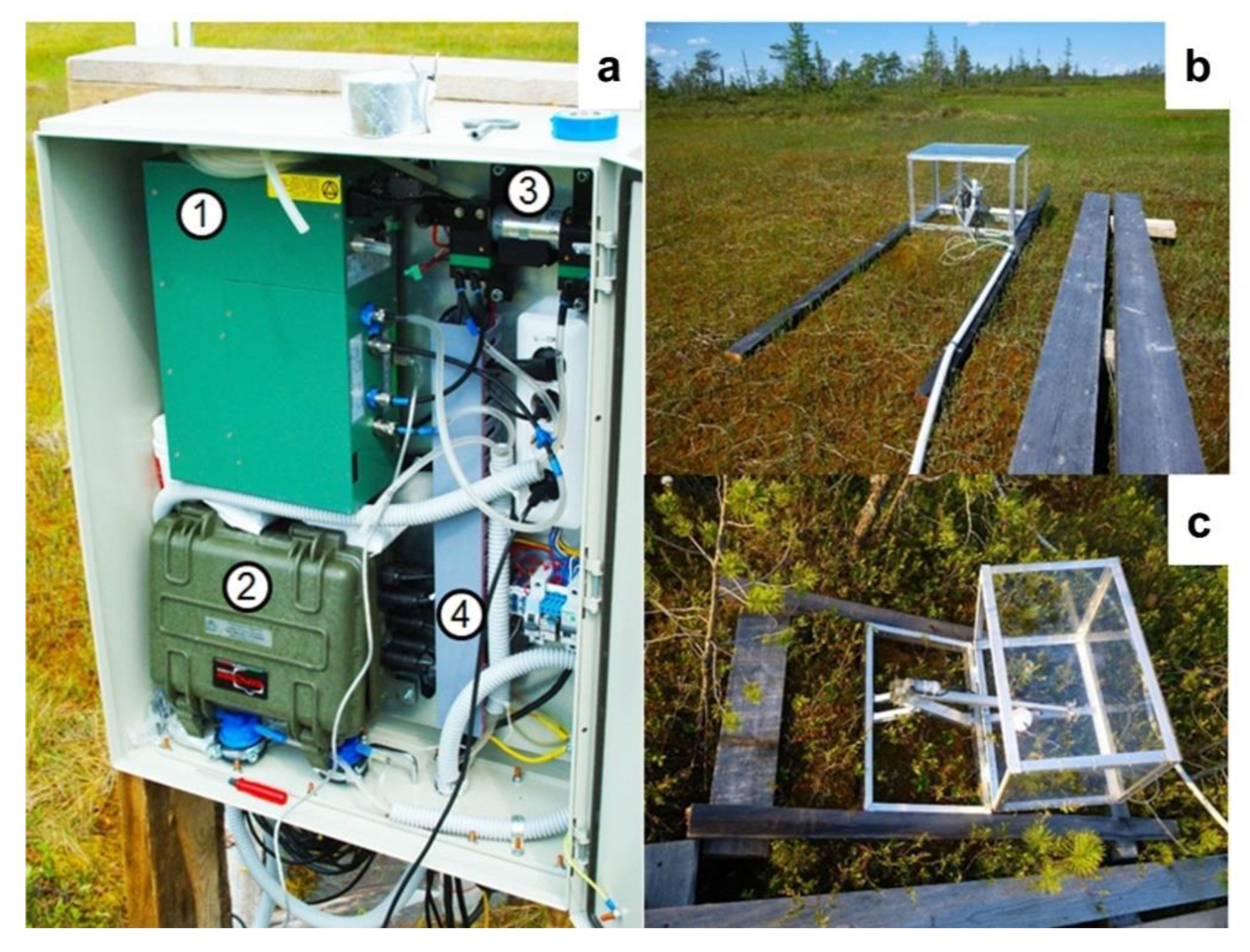
65]. Chamber observation results represent an estimation of GHG fluxes at the local scale. Each chamber plot characterizes a certain form of local peatland microrelief (ridge, hummock, lawn, hollow, pond) with a specific vegetation type. An automated chamber system allows the dynamics of carbon exchange to be studied at a high temporal resolution for extended periods at the local scale [68]. In combination with the appropriate sample allocations, chamber methods are adaptable for the study of the carbon exchange processes at the ecosystem scale [67].
Both EC system and transparent chamber register NEE—a dynamic balance between photosynthetic fixation of CO2 from the atmosphere (GPP) and losses of CO2 by soil and vegetation respiration combining into ER. According to chamber observations, ecosystem respiration rates reached their maximum values in July (55.8 gC m−2 at ridge sites and 98.1 gC m−2 at hollow sites) and minimum values in May (21.4 gC m−2 at hollows and 41.5 gC m−2 at ridge sites). GPP reached the maximum rates in July (−117 gC m−2 at the ridge and −73.7 gC m−2 at the hollow sites). The maximal carbon uptake occurred in July at both sites (−27.2 and −28.4 gC m−2 for the hollows and ridges, respectively). Positive NEE values (up to 22.9 gC m−2) were obtained for September-October at the ridge site. The growing season (May-October) cumulative NEE, calculated by integrating the monthly averaged diurnal NEE rates at the hollow site, was−110, −107.8 and −57.8 gC m−2 in 2017, 2018 and 2019, respectively. Our results show that the amount of CO2 captured from the atmosphere at the ridge site was lower. resulting in −22 and −32.1 gC m−2 in 2018 and 2019. A net CO2 emission of 13.4 gC m−2 was observed at the ridge site in 2017.
A comparison of NEE estimates obtained through EC measurements in 2015 with NEE data from chamber observations shows that EC data are 1.8–3.5 times higher than NEE obtained at the hollow site due to the impact of pine tree photosynthesis, which is not registered by the chamber method. The cumulative May-August NEE from EC measurements was −202 gC m−2 in 2015, with the monthly cumulative values being −35, −72, −79 and −16 gC m−2 month−1 for May-August, respectively. The May-August cumulative NEE splits into ER = 157 g C m−2 and GPP = 359 g C m−2.
Combining EC and chamber observations can provide additional details about the input of peatland tree layers into carbon cycling. The proper estimates of CO2 assimilation by trees require detailed maps of micro landscapes within the EC footprint area and simultaneous observations by EC and chamber methods.
Carbon fluxes essentially depend on meteorological conditions, energy, and water cycles characterized by a high temporal variability. Spatially distributed observations of meteorological and hydrological parameters are required for assessments of factors controlling peatland carbon balance.
The climate conditions of the Mukhrino bog location are continental, with an average annual temperature of −1.0 °C, mean monthly temperatures in July of 17.4 °C, and in January of −21.5 °C. The total amount of precipitation is 470 ± 68 mm, where 25% is snow (~126 mm). Snow melting starts at the end of April and significantly increases the peatland water level. During the summer season, peatland water level slowly drops down with a short-term rise as a response to rainfall. Due to the intensification of the autumn precipitation and decrease in the air temperature and evapotranspiration, a peatland’s water level increases in September. Discharge completely stops at the end of September, beginning in October when the permanent snow cover appears.
The photosynthesis of peatland vegetation is greatly influenced by high-frequency variation in solar radiation [69] and by changes in the groundwater table [70,71]. Sphagnum mosses completely cover the surface of the Mukhrino peatland and provide an important input into the carbon cycle. The share of moss cover in total above-ground net primary production is about 53–63% [29]. The linear annual Sphagnum growth varied from 1.5 to 3.6 cm depending on the species in 2019–2020, and from 0.7 to 3.5 cm in 2013–2015 [54]. Considering the density of the top moss layer and carbon content allows the annual net primary production of Sphagnum mosses to be determined. The net annual accumulation of carbon in the live part of mosses was estimated at 24–190 gC m−2 depending on the species of Sphagnum moss. This estimate can vary significantly depending on the annual precipitation and water table level [54].
The expenditure part of the carbon cycle, due to peat decomposition, is highly dependent on rapid changes in peat surface temperature and on the slower changes in temperature and moisture content of the deeper peat [72]. Mass loss of plant remains through decomposition gives a valuable measurement of net carbon loss, which can be useful for comparing ecosystem or litter substrates. Carbon withdrawal occurs through gaseous emissions of carbon dioxide or methane into the atmosphere or bog water, and through dissolved or particular organic carbon removal with running water [72]. According to our assessments up to 86% (Rubus chamaemorus) of plant remains were removed from the peat after the first four years of decomposition. Sphagnum mosses are more resistant to decomposition, and therefore from 24% (S. balticum) to 48% (S. fuscum) of initial weight was lost over 4 years. Assuming that the total carbon fixed by mosses during the photosynthesis directly enters peat formation allows the maximum carbon accumulation in peat due to Sphagnum mosses to be estimated. The maximal annual carbon accumulation in peat varied from 27 to 100 gC m−2 yr−1 for S. fuscum and from 18 to 80 gC m−2 yr−1 for S. balticum. These values are difficult to interpret because they do not include the input of carbon from other plant species and partial decomposition of dead standing plants before coming to the peatland surface. On another hand, these data do not interfere with the observed long-term carbon accumulation rates obtained by radiocarbon analysis, ranging from 28.5 to 57.2 gC m−2 yr−1 with local extremes of up to 176.2 gC m−2 yr−1.

5. Current Challenges and Future Development

Global climate warming requires close scientific attention, an adaptation of society, social services and institutions, and urges the development of a mitigation program to reduce the anthropogenic impact on the natural ecosystems [15,73]. The Russian Federation initiated a pilot project directed at controlling GHG emissions, including as a part of all activities creating the “carbon polygons” network [74]. It aims to assess the carbon fluxes from both natural and anthropogenically influenced ecosystems, and to develop a comprehensive methodology of carbon balance measurements. The Mukhrino FS has one of the longest available continuously acquired datasets on the fluxes of carbon dioxide in West Siberia. Together with the existing scientific infrastructure, long-term data on biodiversity and environmental conditions, and international experience, it may provide unique information to the government initiative.
Native peatlands are vulnerable to carbon loss under increasing temperatures and frequency of drought events; large uncertainties prevail in the future carbon budget of peatlands and its feedback to climate change [75]. GHG flux data from the Mukhrino FS provide representative results for the taiga zone covering about one third of the West Siberian area. So far, the available data on GHG fluxes covers several seasons and reveals an emission dynamics for the pristine peatland with relation to various microtopes (hollow, ridge, lawn). Future work involves expanding the existing observation network to cover the typical ryam and mixed forest ecosystems by eddy-covariance towers.
An analysis of the obtained results on meteorological and hydrological parameter variability, the spatial structure of the studied peatland, and various components of the peatland carbon cycle, revealed knowledge gaps in the organized monitoring system at the Mukhrino FS. Routine surveys of vegetation productivity are needed to describe the temporal and spatial variability of the incoming part of the carbon cycle. Hydrological studies should be extended by monitoring carbon-containing gases and dissolved and particulate carbon transport with moving water in peatlands, outgoing rivers, and creeks. Full peatland carbon balance accounting requires the monitoring of methane emissions from the peatland surface and lakes. The studied peatland has a complex structure with a high diversity of landscape units. Therefore, the expansion of the carbon flux monitoring network will provide new data for correct carbon balance assessment for ecosystems not yet covered by the EC tower footprint.
Biodiversity, global climate change, and environmental dynamics require a multi-proxy research approach to discover the complex linkages between the ecosystem elements [36]. Thus, the actual scientific challenge is to organize a platform to facilitate access for diverse researchers in studying the objective. The Mukhrino FS provides all-year-around access to the scientific infrastructure and allows long-term experiments to be carried out and data collecting to be integrated into BigData. This advances research from the descriptive level to the level of understanding ecosystem functioning.
Another challenge is that peatlands are increasingly under pressure from human activities related to the exploitation of gas and oil. Such infrastructure can have a profound impact on the environment in and surrounding peatlands [76]. Environmental changes may, via hydrology and changes in soil characteristics, have a large impact on the functioning of natural peatlands and cause significant degradation. To what extent such activities affect peatland functioning, and whether peatlands can adapt to such changes, remains an open question.

6. Conclusions

Placed in the middle taiga zone, thousands of km’s from other observatories and in a peat-rich area, the long-term Mukhrino field station provides unique data on peatland functioning in an undisturbed state. The reported data on peatland climate, hydrology, biodiversity, and carbon balance are useful for the development of a comprehensive model forecasting peatland functioning and carbon cycling linked to climate change, which provides necessary information for carbon emission control and decision making in a field of adaptation to global environmental changes.
Carbon dioxide fluxes are controlled by a set of environmental characteristics, most of which have an essential temporal and spatial variability. Nonlinear relations between environmental characteristics and carbon dioxide fluxes require results of continuous monitoring of meteorological and hydrological variables for the development of mathematical models of carbon exchange in the peat–water–vegetation–atmosphere system. Quantitative links between climate change and carbon processes can be established using mathematical models to forecast future carbon cycle processes and the development of the Earth’s climate system. The obtained estimates of various carbon fluxes using EC and chamber methods, accounting for Sphagnum growth and decomposition, and long-term peat accumulation, provide information about the functioning of the peatland ecosystems at different spatial and temporal scales. Multiscale carbon flux monitoring allows new useful information to be obtained for forecasting the responses of the northern peatland carbon cycle to climatic changes. The main activities are related to field work at the MFS in Western Siberian, with national, and international collaboration and facilitating the external research projects and hosting the active scientific groups. To foster interactions between scientists, and to create a West Siberian science cluster, a traditional International Field Symposium “West Siberian Peatlands and Carbon Cycle: Past and Present” was initiated in 2001. It usually takes place every four years and gathers people from all around the world to exchange knowledge and to discuss the actual issues of peatland studies. To collect valuable science results on nature studies an “Environmental dynamic and global climate changes” journal was organized in 2008. This is a scientific academic peer-review journal published twice a year [77].

Author Contributions

Conceptualization, E.L. and T.V.; methodology, N.F., W.B., E.D., E.Z., J.N., P.A., I.M., G.G., A.M.; software, E.Z., I.F., E.D., P.A.; investigation, N.F., E.D., E.Z., P.A., G.G., A.M., V.K.; writing—original draft preparation, E.Z., E.D.; writing—review and editing, E.L., T.V., W.B., J.N., I.M., V.K., E.D., E.Z., N.F., I.F.; visualization, E.Z., E.D., P.A., I.F.; supervision, E.L. and T.V. All authors have read and agreed to the published version of the manuscript.

Funding

The research was carried out with a grant from the Tyumen region Government in accordance with the program of the West Siberian Interregional Scientific and Educational Centre (National Project “Nauka”), and was supported by Yugra State University grant №17-02-07/58, by RFBR and CNRS according to the research project №21-54-15012. Pavel Alekseychik acknowledges support of the projects CLIMOSS (Climate impacts of boreal bryophytes—from functional traits to global models) funded by the Academy of Finland, Decision no. 296116), and SOMPA (Novel soil management practices—key for sustainable bioeconomy and climate change mitigation), funded by the Strategic Research Council at the Academy of Finland, Decision no. 312912.

Institutional Review Board Statement

Not applicable.

Informed Consent Statement

Not applicable.

Data Availability Statement

All measurements data are available via the open-source DEMIS-SDR (Dynamic Ecological Information Management System—Site and dataset registry) web-portal: https://deims.org/5eddca9f-d876-4e2b-b7c1-f7f13010a0ca, accessed on 1 August 2021.

Acknowledgments

We kindly appreciate to Aleksey Dmitrichenko, who immensely helped and inspired us on all stages of article preparation.

Conflicts of Interest

The authors declare no conflict of interest. The funders had no role in the design of the study; in the collection, analyses, or interpretation of data; in the writing of the manuscript, or in the decision to publish the results.

Appendix A

Figure A1. Overview of automated chamber system at the MFS. (a): Main unit; 1, gas analyser unit (Licor 7000); 2, controlling, logging and remote access unit; 3, pump; 4, power unit. (b): Chamber at the hollow site. (c): Chamber at the ridge site.
Land 10 00824 g0a1
Figure A2. (A): Map showing the Mukhrino station location. (B): photo of the EC tower facing southwest. (C): Digital elevation map based on drone survey. (D): Surface-type classification map. (D) includes an eddy covariance footprint overlay, with the isolines giving the 70% cumulative EC source zone in the three stability classes. Colour coding in (D) is as follows: dark green = ridges-hummocks, light green = lawns-hollows, dark blue = ponds. The red cross marks the location of the EC tower. Adapted from [26].
Land 10 00824 g0a2
Table A1. List of sensors, parameters and installation site at Mukhrino field station, 2010–2019.
nParameterEquipmentRidgeHollow
1Air temperature and humidity at 2 mRotronic HC2A-S311
2Atmospheric pressureCampbell Scientific CS105 PTB101b1-
3Wind speed and direction at 2 mYoung Wind Monitor 05103-1
4Wind speed and direction at 10 mYoung Wind Monitor 051031-
5Incoming PARLi-Cor LI-190R11
6Reflected PARLi-Cor LI-190R11
7Net radiation balanceKipp & Zonen NRLite11
8Ground heat fluxHukseflux Heat Flux Sensor HFP01SC21
9Precipitation (summer)HOBO Data Logging Rain Gauge RG3-M-1
10Snow depthManual observations-1
11Surface albedoCalculated from Li-Cor LI-190R11
Table A2. Number of plots and total number of measurements made in 2019 and 2020 for monitoring of Sphagnum annual growth in Mukhrino field station.
SpeciesNumber of Plots20192020
1Sphagnum angustifolium32727
2Sphagnum balticum32 (30 in OTC)150 (130 in OTC)248 (238 in OTC)
3Sphagnum capillifolium21920
4Sphagnum fuscum43436
5Sphagnum jensenii65456
6Sphagnum divinum42828
7Sphagnum majus21917
8Sphagnum papillosum43435
Total number of measurements57365467
Table A3. Total number of extracted litter bags of each type in decomposition dynamics experiment in Mukhrino FS by decomposition periods and years of installation extracted by spring 2021.
Year of Installation20162017201820192020
Decomposition Period, Months/Substrate312243648312243612243123
Andromeda polifolia 86 8
Betula pubescence 8878 88987 8
Carex limosa 8842 87887 7
Chamaedaphne calyculata 8875 88887 6
Eriophorum vaginatum 8864 88786 8
Ledum palustre 8885 84687 8
Pinus sibirica 8888 88787 8
Populus tremula 8888 88787 8
Rubus chamaemorus 8886 88687 7
Scheuchzeria palustris 862 888
Sphagnum balticum 8841 88987 8
Sphagnum fuscum 8888 88788 8
Tea, green24242423 6460548 78 24
Tea, rooibos24242424 5956538 76 24
Table A4. Total number of extracted bags in decomposition experiment in Mukhrino by vegetation types and under experimental warming conditions extracted by spring 2021.
Vegetation Type/SubstrateA. polifolia LeavesB. pubescence LeavesC. limosa LeavesCh. calyculata LeavesE. vaginatum LeavesL. palustreP. sibirica LeavesP. tremula LeavesR. chamaemorus LeavesS. palustrisS. balticum Green PartsS. fuscum Green PartsTea, GreenTea, Rooibos
Coniferous forest 79 7879 6774
Deciduous forest 10 years after cut 3937
Deciduous forest 40 years after cut 3231
Raised bog lawn 66 71 4069 4040
Raised bog ryam22 173 70 74 794452
OTC dry, chamber 3231
OTC dry, control 3232
OTC wet, chamber 3132
OTC wet, control 3319

References

  1. Berglund, B.E. Human impact and climate changes—Synchronous events and a causal link? Quart. Int. 2003, 105, 7–12. [Google Scholar] [CrossRef]
  2. Joosten, H. Peatlands, Climate Change Mitigation and Biodiversity Conservation: An Issue Brief on the Importance of Peatlands for Carbon and Biodiversity Conservation and the Role of Drained Peatlands as Greenhouse Gas Emission Hotspots; Nordic Council of Ministers: København, Denmark, 2015. [Google Scholar]
  3. Callaghan, T.V.; Kulikova, O.; Rakhmanova, L.; Topp-Jorgensen, E.; Labba, N.; Kuhmanenm, L.-A.; Kirpotin, S.; Shaduyko, O.; Burgess, H.; Rautio, A.; et al. Improving dialogue among researchers, local and indigenous peoples and decision-makers to address issues of climate change in the North. Ambio 2020, 49, 1161–1178. [Google Scholar] [CrossRef] [Green Version]
  4. Tsyganov, A.N.; Zarov, E.A.; Mazei, Y.A.; Kulkov, M.G.; Babeshko, K.V.; Yushkovets, S.Y.; Payne, R.J.; Ratcliffe, J.L.; Fatyunina, Y.A.; Zazovskaya, E.P.; et al. Key periods of peatland development and environmental changes in the middle taiga zone of Western Siberia during the Holocene. Ambio 2021. [Google Scholar] [CrossRef]
  5. Gorham, E. Northern peatlands: Role in the carbon cycle and probable responses to climatic warming. Ecol. Appl. 1991, 1, 182–195. [Google Scholar] [CrossRef]
  6. Charman, D.J.; Beilman, D.W.; Blaauw, M.; Booth, R.K.; Brewer, S.; Chambers, F.M.; Christen, J.A.; Gallego-Sala, A.; Harrison, S.P.; Hughes, P.D.M.; et al. Climate-related changes in peatland carbon accumulation during the last millennium. Biogeosciences 2013, 10, 929–944. [Google Scholar] [CrossRef] [Green Version]
  7. Dise, N.B. Environmental science. Peatland response to global change. Science 2009, 326, 810–811. [Google Scholar] [CrossRef] [PubMed]
  8. Xu, J.; Morris, P.J.; Liu, J.; Holden, J. PEATMAP: Refining estimates of global peatland distribution based on a meta-analysis. Catena 2018, 160, 134–140. [Google Scholar] [CrossRef] [Green Version]
  9. Sheng, Y.; Smith, L.C.; MacDonald, G.M.; Kremenetski, K.V.; Frey, K.E.; Velichko, A.A.; Lee, M.; Beilmannr, D.W.; Dubinin, P.A. High-resolution GIS-based inventory of the west Siberian peat carbon pool. Glob. Biogeochem. Cycl. 2014, 18, GB3004. [Google Scholar] [CrossRef]
  10. Bubier, J.L.; Bhatia, G.; Moore, T.R.; Roulet, N.T.; Lafleur, P.M. Spatial and temporal variability in growing-season net ecosystem carbon dioxide exchange at a large peatland in Ontario, Canada. Ecosystems 2003, 6, 353–367. [Google Scholar]
  11. Olchev, A.; Novenko, E.; Desherevskaya, O.; Krasnorutskaya, K.; Kurbatova, J. Effects of climatic changes on carbon dioxide and water vapor fluxes in boreal forest ecosystems of European part of Russia. Environ. Res. Lett. 2009, 4, 045007. [Google Scholar] [CrossRef]
  12. Golovatskaya, E.A.; Dyukarev, E.A. The influence of environmental factors on the CO2 emission from the surface of oligotrophic peat soils in West Siberia. Eurasian Soil Sci. 2012, 45, 588–597. [Google Scholar] [CrossRef]
  13. Helfter, C.; Campbell, C.; Dinsmore, K.J.; Drewer, J.; Coyle, M.; Anderson, M.; Skiba, U.; Nemitz, E.; Sutton, M.A. Drivers of long-term variability in CO2 net ecosystem exchange in a temperate peatland. Biogeosciences 2015, 12, 1799–1811. [Google Scholar] [CrossRef] [Green Version]
  14. Saunois, M.; Bousquet, P.; Poulter, B.; Peregon, A.; Ciais, P.; Canadell, J.G.; Dlugokencky, E.J.; Etiope, G.; Bastviken, D.; Houweling, S.; et al. The global methane budget 2000–2012. Earth Syst. Sci. Data 2016, 8, 697–751. [Google Scholar] [CrossRef] [Green Version]
  15. IPCC. Contribution of Working Groups I, II and III to the Fifth Assessment Report of the Intergovernmental Panel on Climate Change. In Climate Change: Synthesis Report; IPCC: Geneva, Switzerland, 2014; p. 151. [Google Scholar]
  16. Naumov, A.V. Soil Respiration; Izd SO RAN: Novosibirsk, Russia, 2009; pp. 1–208. [Google Scholar]
  17. Sasakawa, M.; Ito, A.; Machida, T.; Tsuda, N.; Niwa, Y.; Davydov, D.; Fofonov, A.; Arshinov, M. Annual variation of CH4 emissions from the middle taiga in West Siberian Lowland (2005–2009): A case of high CH4 flux and precipitation rate in the summer of 2007. Tellus B Chem. Phys. Meteorol. 2012, 64, 17514. [Google Scholar] [CrossRef]
  18. Molchanov, A.G.; Olchev, A.V. Model of CO2 exchange in a sphagnum peat bog. Comput. Res. Model. 2016, 8, 369–377. [Google Scholar] [CrossRef]
  19. Leroy, F.; Gogo, S.; Guimbaud, C.; Bernard-Jannin, L.; Hu, Z.; Laggoun-Défarge, F. Vegetation composition controls temperature sensitivity of CO2 and CH4 emissions and DOC concentration in peatlands. Soil Biol. Biochem. 2017, 107, 164–167. [Google Scholar] [CrossRef] [Green Version]
  20. Veretennikova, E.E.; Dyukarev, E.A. Diurnal variations in methane emissions from West Siberia peatlands in summer. Russ. Meteorol. Hydrol. 2017, 42, 319–326. [Google Scholar] [CrossRef]
  21. Veretennikova, E.E.; Dyukarev, E.A. Spatial and temporal dynamics of methane fluxes from the bog ecosystems of the southern taiga of Western Siberia. Boreal Environ. Res. 2021, 26, 43–59. [Google Scholar] [CrossRef]
  22. Kirpotin, S.N.; Callaghan, T.V.; Peregon, A.M.; Babenko, A.S.; Berman, D.I.; Bulakhova, N.A.; Byzaakay, A.A.; Chernykh, T.M.; Chursin, V.; Interesova, E.A.; et al. Impacts of environmental change on biodiversity and vegetation dynamics in Siberia. Ambio 2021. [Google Scholar] [CrossRef] [PubMed]
  23. The Data Portal Serving the FLUXNET Community. Available online: https://fluxnet.org (accessed on 25 July 2021).
  24. Pallandt, M.; Kumar, J.; Mauritz, M.; Schuur, E.; Virkkala, A.-M.; Celis, G.; Hoffman, F.; Göckede, M. Representativeness assessment of the pan-Arctic eddy-covariance site network, and optimized future enhancements. Biogeosci. Discuss. 2021. [Google Scholar] [CrossRef]
  25. Lappalainen, H.K.; Kerminen, V.-M.; Petäjä, T.; Kurten, T.; Baklanov, A.; Shvidenko, A.; Bäck, J.; Vihma, T.; Alekseychik, P.; Arnold, S.; et al. Pan-Eurasian Experiment (PEEX): Towards holistic understanding of the feedbacks and interactions in the land–atmosphere–ocean–society continuum in the Northern Eurasian region. Atmos. Chem. Phys. 2016, 16, 14421–14461. [Google Scholar] [CrossRef] [Green Version]
  26. Park, S.-B.; Knohl, A.; Lucas-Moffat, A.M.; Migliavacca, M.; Gerbig, C.; Gerbiga, C.; Vesala, T.; Peltola, O.; Mammarella, I.; Kolle, O.; et al. Strong radiative effect induced by clouds and smoke on forest net ecosystem productivity in central Siberia. Agric. For. Meteorol. 2018, 250–251, 376–387. [Google Scholar] [CrossRef]
  27. Sasakawa, M.; Machida, T.; Ishijima, K.; Arshinov, M.; Patra, P.K.; Ito, A.; Aoki, S.; Petrov, V. Temporal Characteristics of CH4 Vertical Profiles Observed in the West Siberian Lowland Over Surgut from 1993 to 2015 and Novosibirsk from 1997 to 2015. J. Geophys. Res. Atmos. 2017, 122, 11261–11273. [Google Scholar] [CrossRef]
  28. Davydov, D.K.; Dyachkova, A.V.; Fofonov, A.V.; Maksyutov, S.S.; Dyukarev, E.A.; Smirnov, S.V.; Glagolev, M.V. Measurements of methane and carbon dioxide fluxes from wetland ecosystems of the Southern Taiga of West Siberia. Proc. SPIE 2018, 10833, 1083389. [Google Scholar] [CrossRef]
  29. Golovatskaya, E.A.; Dyukarev, E.A. Carbon budget of oligotrophic bog in southern taiga in Western Siberia. Plant Soil 2009, 315, 19–34. [Google Scholar] [CrossRef]
  30. Kharanzhevskaya, Y.A.; Voistinova, E.S.; Sinyutkina, A.A. Spatial and temporal variations in mire surface water chemistry as a function of geology, atmospheric circulation and zonal features in the south-eastern part of Western Siberia. Sci. Total Environ. 2020, 733, 139344. [Google Scholar] [CrossRef]
  31. Karlsson, J.; Serikova, S.; Vorobyev, S.N.; Rocher-Ros, G.; Denfeld, B.; Pokrovsky, O.S. Carbon emission from Western Siberian inland waters. Nat. Commun. 2021, 12, 825. [Google Scholar] [CrossRef]
  32. Sabrekov, A.F.; Runkle, B.R.K.; Glagolev, M.V.; Terentieva, I.E.; Stepanenko, V.M.; Kotsyurbenko, O.R.; Maksyutov, S.S.; Pokrovsky, O.S. Variability in methane emissions from West Siberia’s shallow boreal lakes on a regional scale and its environmental controls. Biogeosciences 2017, 14, 3715–3742. [Google Scholar] [CrossRef] [Green Version]
  33. Terentieva, I.E.; Sabrekov, A.F.; Ilyasov, D.; Ebrahimi, A.; Glagolev, M.V.; Maksyutov, S. Highly dynamic methane emission from the west siberian boreal floodplains. Wetlands 2019, 39, 217–226. [Google Scholar] [CrossRef]
  34. Terent’eva, I.E.; Sabrekov, A.F.; Glagolev, M.V.; Lapshina, E.D.; Smolentsev, B.A.; Maksyutov, S.S. A new map of wetlands in the southern taiga of the West Siberia for assessing the emission of methane and carbon dioxide. Water Resour. 2017, 44, 297–307. [Google Scholar] [CrossRef]
  35. Shevchenko, V.P.; Pokrovsky, O.S.; Vorobyev, S.N.; Krickov, I.V.; Manasypov, R.M.; Politova, N.V.; Kopysov, S.G.; Dara, O.M.; Auda, Y.; Shirokova, L.S.; et al. Impact of snow deposition on major and trace element concentrations and elementary fluxes in surface waters of the Western Siberian Lowland across a 1700 km latitudinal gradient. Hydrol. Earth Syst. Sci. 2017, 21, 5725–5746. [Google Scholar] [CrossRef] [Green Version]
  36. Kirpotin, S.N.; Antoshkina, O.A.; Berezin, A.E.; Elshehawi, S.; Feurdean, A.; Lapshina, E.D.; Pokrovsky, O.S.; Peregon, A.M.; Semenova, N.M.; Tanneberger, F.; et al. Great Vasyugan Mire: How the world’s largest peatland helps addressing the world’s largest problems. Ambio 2021. [Google Scholar] [CrossRef]
  37. Ivanov, K.E.; Novikov, S. Mires of Western Siberia, Their Structure and Hydrological Regime; Nauka: Moscow, Soviet Union, 1976; p. 447. [Google Scholar]
  38. Bleuten, W.; Zarov, E.; Schmitz, O. A high-resolution transient 3-dimensional hydrological model of an extensive undisturbed bog complex in West Siberia. Mires Peat 2020, 26, 1–25. [Google Scholar]
  39. Terentieva, I.E.; Glagolev, M.V.; Lapshina, E.D.; Sabrekov, A.F.; Maksyutov, S.S. Mapping of West Siberian taiga wetland complexes using Landsat imagery: Implications for methane emissions. Biogeosciences 2016, 13, 4615–4626. [Google Scholar] [CrossRef] [Green Version]
  40. Photos of the Peatland Landscape. Available online: https://www.flickr.com/photos/mukhrinostation/albums/72157632674684023 (accessed on 1 August 2021).
  41. Dyukarev, E.; Filippova, N.; Karpov, D.; Shnyrev, N.; Zarov, E.; Filippov, I.; Voropay, N.; Avilov, V.; Artamonov, A.; Lapshina, E. Hydrometeorological dataset of West Siberian boreal peatland: A 10-year records from the Mukhrino field station. Earth Syst. Sci. Data 2021, 13, 2595–2605. [Google Scholar] [CrossRef]
  42. Mukhrino Field Station of Yugra State University—Russian Federation. Dynamic Ecological Information Management System—Site and Dataset Registry Web-Portal. Available online: https://deims.org/5eddca9f-d876-4e2b-b7c1-f7f13010a0ca (accessed on 1 May 2021).
  43. Dyukarev, E.; Filippova, N.; Karpov, D.; Shnyrev, N.; Zarov, E.; Filippov, I.; Voropay, N.; Avilov, V.; Artamonov, A.; Lapshina, E. Hydrometeorological dataset of West Siberian boreal peatland: A 10-year records from the Mukhrino field station. (Version 2020/12) [Dataset]. Zenodo 2020. [Google Scholar] [CrossRef]
  44. Nijp, J.J.; Metselaar, K.; Limpens, J.; Bartholomeus, H.M.; Nilsson, M.B.; Berendse, F.; Van der Zee, S.E. High-resolution peat volume change in a northern peatland: Spatial variability, main drivers, and impact on ecohydrology. Ecohydrology 2019, 12, e2114. [Google Scholar] [CrossRef] [Green Version]
  45. Bleuten, W.; Filippov, I. Hydrology of mire ecosystems in central West Siberia: The Mukhrino field station. Dyn. Environ. Glob. Clim. Chang. 2008, 1, 208–224. [Google Scholar] [CrossRef] [Green Version]
  46. Dyukarev, E.A. Partitioning of net ecosystem exchange using chamber measurements data from bare soil and vegetated sites. Agric. For. Meteorol. 2017, 239, 236–248. [Google Scholar] [CrossRef]
  47. Dyukarev, E.; Godovnikov, E.; Karpov, D.; Kurakov, S.; Lapshina, E.; Filippov, I.; Filippova, N.; Zarov, E. Net ecosystem exchange, gross primary production and ecosystem respiration in ridge-hollow complex at Mukhrino bog. Geogr. Environ. Sustain. 2019, 12, 227–244. [Google Scholar] [CrossRef]
  48. Alekseychik, P.; Mammarella, I.; Karpov, D.; Dengel, S.; Terentieva, I.; Sabrekov, A.; Glagolev, M.; Lapshina, E. Net ecosystem exchange and energy fluxes measured with eddy covariance technique in a West Siberian bog. Atmos. Chem. Phys. 2017, 17, 9333–9345. [Google Scholar] [CrossRef] [Green Version]
  49. Mammarella, I.; Peltola, O.; Nordbo, A.; Järvi, L.; Rannik, Ü. Quantifying the uncertainty of eddy covariance fluxes due to the use of different software packages and combinations of processing steps in two contrasting ecosystems. Atmos. Meas. Tech. 2016, 9, 4915–4933. [Google Scholar] [CrossRef] [Green Version]
  50. Sabbatini, S.; Mammarella, I.; Arriga, N.; Fratini, G.; Graf, A.; Hörtnagl, L.; Ibrom, A.; Longdoz, B.; Mauder, M.; Merbold, L.; et al. Eddy covariance raw data processing for CO2 and energy flux calculation at ICOS ecosystem stations. Int. Agrophys. 2018, 32, 495–515. [Google Scholar] [CrossRef]
  51. Kosykh, N.P.; Vishnyakova, E.K.; Koronatova, N.G.; Sayb, E.A.; Filippova, N.V. Production and destruction processes in oligotrophic hollows in the middle taiga (OTC-experiment). In Carbon Balance of Western Siberia Peatlands in the Context of Climate Change, Proceedings of the International Conference, Khanty-Mansiysk, Russia, 19–29 June 2017; Lapshina, E.D., Mironycheva-Tokareva, N.P., Eds.; Publishing house of Tomsk State Univ.: Tomsk, Russia, 2017; pp. 77–79. [Google Scholar]
  52. Delarue, F.; Buttler, A.; Bragazza, L.; Grasset, L.; Jassey, V.E.; Gogo, S.; Laggoun-Défarge, F. Experimental warming differentially affects microbial structure and activity in two contrasted moisture sites in a Sphagnum-dominated peatland. Sci. Total Environ. 2015, 511, 576–583. [Google Scholar] [CrossRef] [Green Version]
  53. Filippova, N.; Kosykh, N. Sphagnum Annual Growth in Mukhrino Field Station, West Siberia. Version 1.5. Yugra State University Biological Collection (YSU BC). Sampling Event Dataset. Available online: https://www.gbif.org/dataset/fae98fd0-c0a2-460f-a30c-53cb4c88006c (accessed on 1 February 2021).
  54. Kosykh, N.P.; Koronatova, N.G.; Lapshina, E.D.; Filippova, N.V.; Vishnyakova, E.K.; Stepanova, V.A. Linear growth and production of Sphagnum mosses in the middle taiga zone of West Siberia. Environ. Dyn. Glob. Clim. Chang. 2017, 8, 3–13. [Google Scholar] [CrossRef]
  55. Keuskamp, J.A.; Dingemans, B.J.; Lehtinen, T.; Sarneel, J.M.; Hefting, M.M. Tea Bag Index: A novel approach to collect uniform decomposition data across ecosystems. Methods Ecol. Evol. 2013, 4, 1070–1075. [Google Scholar] [CrossRef]
  56. Djukic, I.; Kepfer-Rojas, S.; Schmidt, I.K.; Larsen, K.S.; Beier, C.; Berg, B.; Verheyen, K.; Caliman, A.; Paquette, A.; Gutiérrez-Girón, A. Early stage litter decomposition across biomes. Sci. Total Environ. 2018, 628, 1369–1394. [Google Scholar] [CrossRef] [PubMed] [Green Version]
  57. MacDonald, E.; Brummell, M.E.; Bieniada, A.; Elliot, J.; Engering, A.; Gauthier, T.L.; Saraswati, S.; Touchette, S.; Tourmel-Coiechesne, L.; Strack, M. Using the Tea Bag Index to characterize decomposition rates in restored peatlands. Boreal Environ. Res. 2018, 23, 221–235. [Google Scholar]
  58. Filippova, N. Decomposition Dynamics of Native and Standard Substrates in Forests and Peatlands: Mukhrino Field Station, Western Siberia. Yugra State University Biological Collection (YSU BC). Occurrence Dataset. Available online: https://www.gbif.org/dataset/54641290-55dd-48d1-a1a7-25d6eee5d714 (accessed on 24 March 2021).
  59. Tolonen, K.; Turunen, J. Accumulation rates of carbon in mires in Finland and implications for climate change. Holocene 1996, 6, 171–178. [Google Scholar] [CrossRef]
  60. QGIS Development Team. QGIS Geographic Information System. Open Source Geospatial Foundation. Available online: http://qgis.org (accessed on 1 August 2021).
  61. GRASS Development Team. GRASS 6.4 Users Manual. Open Source Geospatial Foundation, USA. Available online: http://grass.osgeo.org/grass64/manuals/ (accessed on 10 June 2021).
  62. McCauley, J.D.; Engel, B.A. Comparison of Scene Segmentations: SMAP, ECHO and Maximum Likelyhood. IEEE Trans. Geosci. Remote Sens. 1995, 33, 1313–1316. [Google Scholar] [CrossRef]
  63. Yu, Z.; Beilman, D.W.; Frolking, S.; MacDonald, G.M.; Roulet, N.T.; Camill, P.; Charman, D.J. Peatlands and their role in the global carbon cycle. Eos Trans. Amer. Geophys. Union 2011, 92, 97–108. [Google Scholar] [CrossRef]
  64. Lafleur, P.M.; Moore, T.R.; Roulet, N.T.; Frolking, S. Ecosystem respiration in a cool temperate bog depends on peat temperature but not water table. Ecosystems 2005, 8, 619–629. [Google Scholar] [CrossRef]
  65. Rebmann, C.; Aubinet, M.; Schmid, H.; Arriga, N.; Aurela, M.; Burba, G.; Clement, R.; De Ligne, A.; Fratini, G.; Gielen, B.; et al. ICOS eddy covariance flux-station site setup: A review. Int. Agrophys. 2018, 32, 471–494. [Google Scholar] [CrossRef]
  66. Aubinet, M.; Vesala, T.; Papale, D. (Eds.) Eddy Covariance: A Practical Guide to Measurement and Data Analysis; Springer Science & Business Media: Dordrecht, The Netherlands; Heidelberg, Germany; London, UK; New York, NY, USA, 2012. [Google Scholar]
  67. Acosta, M.; Pavelka, M.; Montagnani, L.; Kutsch, W.; Lindroth, A.; Juszczak, R.; Janouš, D. Soil surface CO2 efflux measurements in Norway spruce forests: Comparison between four different sites across Europe-from boreal to alpine forest. Geoderma 2013, 192, 295–303. [Google Scholar] [CrossRef]
  68. Pavelka, M.; Acosta, M.; Kiese, R.; Altimir, N.; Brümmer, C.; Crill, P.; Darenova, E.; Fuß, R.; Gielen, B.; Graf, A.; et al. Standardisation of chamber technique for CO2, N2O and CH4 fluxes measurements from terrestrial ecosystems. Int. Agrophys. 2018, 32, 569–587. [Google Scholar] [CrossRef]
  69. Jassey, V.E.J.; Signarbieux, C. Effects of climate warming on Sphagnum photosynthesis in peatlands depend on peat moisture and species-specific anatomical traits. Glob. Chang. Biol. 2019, 25, 3859–3870. [Google Scholar] [CrossRef] [PubMed]
  70. Juszczak, R.; Augustin, J. Exchange of the greenhouse gases methane and nitrous oxide at a temperate pristine fen mire in Central Europe. Wetlands 2013, 33, 895–907. [Google Scholar] [CrossRef] [Green Version]
  71. Mikhailov, O.A.; Zagirova, S.V.; Miglovets, M.N.; Wille, C. Carbon dioxide fluxes in the ecosystem of meso-oligotrophic peatland during the transition period from autumn to winter. Contemp. Probl. Ecol. 2013, 6, 143–148. [Google Scholar] [CrossRef]
  72. Bell, M.C.; Ritson, J.P.; Verhoef, A.; Brazier, R.E.; Templeton, M.R.; Graham, N.J.D.; Freeman, C.; Clark, J.M. Sensitivity of peatland litter decomposition to changes in temperature and rainfall. Geoderma 2018, 331, 29–37. [Google Scholar] [CrossRef]
  73. Roshydromet. Second Assessment Report of Roshydromet on Climate Change and Its Consequences on the Territory of the Russian Federation; Roshydromet: Russia, Moscow, 2014; pp. 18–235. [Google Scholar]
  74. The Ministry of Education and Science of Russia Will Launch a Program for the Development of Carbon Polygons. Available online: https://www.minobrnauki.gov.ru/press-center/news/?ELEMENT_ID=26691&sphrase_id=102783 (accessed on 11 May 2021).
  75. Wu, Y.; Verseghy, D.L.; Melton, J.R. Integrating peatlands into the coupled Canadian Land Surface Scheme (CLASS) v3.6 and the Canadian Terrestrial Ecosystem Model (CTEM) v2.0. Geosci. Model Dev. 2016, 9, 2639–2663. [Google Scholar] [CrossRef] [Green Version]
  76. Lopatin, K.I.; Kashtanova, O.A.; Montile, A.I. An optimization model for the placement of oilfield facilities in the forest-bog zone of Western Siberia. Bull. Nizhnevartovsk State Univ. 2009, 1, 62–67. (In Russian). Available online: https://vestnik.nvsu.ru/2311-1402/article/view/49061 (accessed on 1 August 2021).
  77. Environmental Dynamics and Global Climate Change. About the Journal. Available online: https://edgccjournal.org/EDGCC/index (accessed on 25 July 2021).
Figure 1. Map of the study region. Location of the Mukhrino field station. (A): On the local scale (1—water, 2—floodplain, 3—ridge-hollow bog, 4—ryam bog, 5—pine forest, 6—mixed forest, 7—deciduous forest, 8—burnt and disturbed forest, 9—infrastructure). (B): On the Russian Federation scale.
Land 10 00824 g001
Figure 2. (A): Sentinel-2 image with B8(NIR)-B11(SWIR)-B4(RED) false color band combination, 15 m spatial resolution. (B): Resurs-P image true color 2 m spatial resolution. 1: Ridge-hollow-pool patterned bogs and water tracks; 1a, Dwarf shrubs-Sphagnum ridges; 1b, Sphagnum lawns; 1c, Water pools and waterlogged hollows. 2: Ridge-hollow patterned bogs; 2a, Pine-dwarf shrubs, Sphagnum ridges; 2b, Sphagnum hollows. 3: Dwarf shrub Sphagnum bog with sparse low pine trees (‘Open bog’). 4: Wooded pine-dwarf shrub-Sphagnum bog (Ryam); 4a, Typical ryam; 4b, Tall ryam; 4c, Ryam with small cotton grass hollows. 5: Sedge-Sphagnum fen (incl. sparse low birch fens). 6: Dark coniferous and mixed forest. 7: Small-leaved forest. 8 and 9: Floodplain willow and meadows. 10: Floodplain sedge wetlands.
Land 10 00824 g002
Figure 3. Location of the monitoring plots and equipment.
Land 10 00824 g003
Figure 4. Meteorological data recorded at the ridge site at MFS. Legend: (a), air temperature (°C); (b), atmospheric pressure (kPa); (c), vapor pressure (kPa); (d), photosynthetically active radiation (µmol m−2 s−1); (e), net radiation (W m−2); (f), soil heat flux (W m−2); (g), wind rose at 10 m; (h), wind rose at 2 m. 1: wind speed = 0.5~2 m s−1. 2: wind speed = 2~ 5 m s−1. 3: wind speed = >5 m s−1. Red line = raw observations, blue line = gap-filled data.
Land 10 00824 g004
Figure 5. Averaged annual water table depth variation for different microtopes, cm. Positive y-values represent water above the surface, negative y-values represent water below the surface. Grey bars represent precipitation in mm. * A piezometer on the ridge was installed in a local depression −25 cm deep.
Land 10 00824 g005
Figure 6. Monthly carbon dioxide fluxes at the ridge and the hollow sites at Mukhrino bog in 2017–2019.
Land 10 00824 g006
Figure 7. Cumulative gap-filled NEE, Re and GPP obtained by the eddy-covariance setup in May–August 2015. Adapted from [48].
Land 10 00824 g007
Figure 8. Mean annual growth increment of Sphagnum for all species cumulatively (A) and individually (B) in two successive years of measurements (2019, 2020).
Land 10 00824 g008
Figure 9. The mean weight loss of different litter types with standard deviation for 1 to 4 years of decomposition.
Land 10 00824 g009
Table 1. Evapotranspiration values for the different microtopes.
MicrotopeEvapotranspiration, mm/day
Hollow7.8 ± 5.1
Ridge7.6 ± 3.9
Ryam *4.3 ± 3.9
Open water7.0 ± 5.1
* Calculation based only on two years of measurements.
Table 2. Annual net ecosystem exchange (gC m−2) values for the ridge and hollow.
Microtope/Year201720182019
Ridge+13.4−22.0−32.1
Hollow−110.0−107.8−57.8
Publisher’s Note: MDPI stays neutral with regard to jurisdictional claims in published maps and institutional affiliations.

