
Investigating Ecosystem Service Trade-Offs/Synergies and Their Influencing Factors in the Yangtze River Delta Region, China

1
Belt & Road Institute, Jiangsu Normal University, Xuzhou 221009, China
2
School of Architecture & Design, China University of Mining and Technology, Xuzhou 221116, China
*
Author to whom correspondence should be addressed.
Land 2022, 11(1), 106; https://0-doi-org.brum.beds.ac.uk/10.3390/land11010106
Submission received: 8 December 2021
/
Revised: 27 December 2021
/
Accepted: 6 January 2022
/
Published: 9 January 2022
Abstract
:A comprehensive understanding of the ecosystem services (ESs) trade-off/synergy relationships has become increasingly important for ecological management and sustainable development. This study employed the Yangtze River Delta (YRD) region in China as the study area and investigated the spatiotemporal changes in three ESs, namely, carbon storage (CS), water purification (WP), and habitat quality (HQ). A trade-off/synergy degree (TSD) indicator was developed that allowed for the quantification of the trade-off/synergy intensity, and the spatial pattern of the TSD between ESs in the YRD region to be analyzed. Furthermore, a geographically weighted regression (GWR) model was used to analyze the relationship between the influencing factors and trade-offs/synergies. The results revealed that CS, WP, and HQ decreased by 0.28%, 2.49%, and 3.38%, respectively, from 2005 to 2015. The TSD indicator showed that the trade-off/synergy relationships and their magnitudes were spatially heterogeneous throughout the YRD region. The coefficients of the natural and socioeconomic factors obtained from the GWR indicated that their impacts on the trade-offs/synergies vary spatiotemporally. The impact factors had both positive and negative effects on the trade-offs/synergies. The findings of this study could improve the understanding of the spatiotemporal dynamics of trade-offs/synergies and their spatially heterogeneous correlations with related factors.
1. Introduction
Ecosystem services (ESs) refer to the products and services obtained from ecosystems. ESs are the basis of human survival and are closely related to human wellbeing. As evidenced by the Millennium Ecosystem Assessment (MEA), the loss of ESs in recent decades directly threatens regional and global ecological security [1], and this worsening trend is likely to continue in the future due to the increasing intensity of human activities [2].
In the process of pursuing socioeconomic benefits, human beings have significant impact on the ESs interactions, which is manifested as the ES trade-off and synergy. The ES trade-off presents a win-lose situation that involves enhancing one ecosystem service at the expense of reducing another, and ES synergy presents a win-win situation that involves the enhancement of multiple ecosystems [3]. The dramatic socioeconomic development leads to an improvement in one ES at the expense of other ESs, thus threatening the stability and security of ecosystems and significantly influencing human wellbeing [4]. Ecosystem management relies on “our best understanding of the ecological interactions and processes necessary to sustain ecosystem composition, structure, and function” [5]. Ecosystem management should not only pursue single ecosystem service benefits but also consider the balance among multiple ESs to maximize the overall benefits and promote regional sustainable development. The importance and urgency of understanding the complex interactions among multiple ESs have been widely recognized by ecosystem managers and researchers [6,7,8]. Many efforts have been made to describe and assess changes in ESs and their complex interactions (trade-offs and synergies) as well as the urbanization process and land cover changes [7,9,10]. Previous studies on ESs found that trade-off relationships are ubiquitous [11,12], for example, they consider the trade-off between services resulting in the provision of a good (food production, wood production) and regulation services (soil conservation, water purification, regional biodiversity maintenance). Prior findings suggest that ecosystem management should coordinate various ESs to promote their overall benefits [13,14].
The identification of the trade-off/synergy relationships that exist between ESs can improve the effectiveness of ecological management [15,16]. Over the past few years, numerous studies on trade-offs/synergies have focused on the identification and expression of the types of relationships that exist between multiple ESs using different methods. At present, research involving a trade-off/synergy analysis is mainly conducted using statistical methods [17,18], spatial mapping [3], and scenario analysis [19,20]. For instance, Braun et al. (2018) applied a Pearson correlation analysis to identify the various types of relationships that exist between ESs [21]; Xu et al. (2018) used spatial overlapping and Spearman’s rank correlation to analyze the relationships among ESs [8]; Kubiszewski et al. (2017) adopted a scenario analysis to determine the trade-offs/synergies that exist between ESs [22]; and Zheng et al. (2016) used radar graphs to represent the trade-off/synergy relationships [9]. These methods have enhanced the understanding of the trade-offs/synergies that exist among ESs. However, qualitative analyses of the trade-off relationships cannot measure the magnitudes of the effects of the related factors on the trade-off/synergy relationship, which is required for effective ecosystem management and planning [23,24]. The potential nonlinear characteristics of the trade-offs/synergies between ESs cannot be adequately addressed using qualitative methods. Therefore, quantitative research is urgently needed to analyze the trade-offs that exist among ESs. Some scholars tried to develop indicators to analyze these trade-offs. Laterra et al. (2012) used the total ecosystem services (TES) index to quantify the interrelationships that exist among multiple ESs [25]; Bradford and D’Amato (2012) used the root mean square error (RMSE), a statistical method, to evaluate the trade-off relationships among multiple ESs [26]. Pan et al. (2013) quantified the trade-off relationships among ESs by proposing the ecosystem trade-off (ETO) index [27]. However, the temporal scale effect of the trade-offs/synergies among ESs was not considered in previous studies. Furthermore, these indicators cannot reveal how the variations in multiple natural and socioeconomic factors affect the interactions between ESs over a specific period. Thus, the quantitative and spatial nature of these trade-offs/synergies is strongly limited. Therefore, it is critical to propose a new indicator for quantifying the intensity of trade-offs/synergies. The spatial differences of trade-offs/synergies intensity could be numerically expressed.
Fully understanding how influencing factors affect ESs and their trade-offs/synergies is a prerequisite for effective and targeted regional planning [28]. Therefore, it is urgent to identify the factors of the interactions that exist among ES’s relationships. By understanding the related factors and their effects on trade-offs/synergies, we can coordinate the trade-offs and improve the synergies between ESs [29]. Several studies have argued that the understanding of ES trade-offs/synergies is insufficient without carefully considering and analyzing the driving mechanisms that underlie ES relationships [30,31]. Although many studies have been carried out to investigate the trade-off and synergy relationships and their spatiotemporal changes, there is still little known about the factors of these complex interactions. The dynamics of ESs and the related trade-off/synergy relationships are complicated processes that involve various natural and socioeconomic variables. In previous studies, the relationships between influencing factors and the associated trade-offs/synergies were commonly analyzed using qualitative methods such as by comparing scenarios [9,10,32]. The question of how and to what extent the influencing factors affect trade-offs/synergies remains poorly understood. To address these gaps, correlation analysis techniques such as Pearson correlation [33], redundancy analysis (RDA) [4], and multivariate regression trees [31] were applied to explain the global relationships among ES trade-offs/synergies and the related factors without considering spatial heterogeneity. It is recognized that the trade-off/synergy relationships among ESs are affected by spatial heterogeneity. For example, in South Africa, a trade-off between carbon sequestration and freshwater supply was found [34], while research on the Baiyangdian River Basin found a synergistic relationship between these two variables [35]. Therefore, it was assumed that the effects of influencing factors on trade-offs/synergies should be spatial heterogeneity, i.e., the variations in the effects over space. Global relationships reveal information only about the average conditions and might consequently overlook location-specific impacts [36,37]. If we ignore spatial heterogeneity, errors might arise in the results of analyses on the impacts of influencing factors on ES interactions, increasing uncertainty about ES management policies [29]. Despite the breadth of previous studies, a key question remains to be answered: how do different natural and socioeconomic factors impact the trade-offs/synergies among ESs with consideration of spatial heterogeneity? The geographical weighted regression (GWR) model is a local regression method that can explore the spatially varying relationship [38,39]. This method could provide more detailed spatial information on the complicated relationship between multiple variables and trade-offs/synergies among ESs.
The YRD region is an economically developed and densely populated area in China that is experiencing serious ecological degradation and environmental pollution. This paper aims at partly address this knowledge gap by using the YRD as the study area and investigating the spatiotemporal changes in the trade-offs/synergies among ESs and their spatial heterogeneous correlation with the related factors. Specifically, the objectives were to: (1) reveal the dynamics of the trade-offs/synergies that exist among ESs in the YRD region by using a new proposed indicator; (2) explore the spatially heterogeneous relationships that exist between the influencing factors and trade-offs/synergies by employing the GWR model; and (3) propose the implications of coordinating ESs to achieve sustainable development for ecosystem management.
2. Materials and Methods
2.1. Study Area
In this paper, the YRD region (115°47′–122°56′ E, 27°55′–34°27′ N) refers to associated urban agglomeration discussed in the “Yangtze River Delta Urban Agglomeration Development Plan” approved by the State Council in May 2016. The YRD region is located in a subtropical monsoon climate zone, with an annual precipitation of 800–2050 mm, presenting significant regional differences. The precipitation decreases from southeast to northwest, and the annual average temperature ranges from 9.3–17.3 °C. As shown in Figure 1, the YRD region includes 26 cities, including Shanghai, Nanjing, Hangzhou, Hefei, etc. The area of the whole region is 211,700 km2, accounting for 2.1% of the total land area of China.
The YRD region is one of the regions with the most rapid economic and urbanization development in China. Changes in land-use have significantly changed the structure and pattern of regional ecosystems, and many ecological environmental risks related to water regulation, air purification, and climate regulation are becoming increasingly severe. The contradiction between regional socioeconomic development and the protection of the ecological environment has become the main limiting factor that restricts the coordinated development of the YRD region and has a certain negative impact on human wellbeing. Due to socioeconomic development and the expansion of cities, the magnitude of ES trade-offs will continue to increase.
Therefore, the quantitative measurement of the spatiotemporal dynamics in the patterns of the trade-offs/synergies in the YRD and the identification of the spatially heterogeneous effects of influencing factors on trade-offs/synergies in the YRD region may not only enrich research on ESs but also provide a scientific basis for optimizing ecosystem management and regional planning.
2.2. Data
The following data were used in this study: (1) land cover data on the YRD region for 2005 and 2015 with a resolution of 30 m, obtained from the Data Centre for Resources and Environmental Sciences, Chinese Academy of Sciences (RESDC) (http://www.resdc.cn/Default.aspx, accessed on 7 June 2021). Land cover was reclassified into six categories based on the data: cultivated land, forestland, grassland, water bodies, built-up land, and unused land. (2) Meteorological data, including information on precipitation, total solar radiation and the temperature in the YRD region from 2005 to 2015, derived from the China Meteorological Data Service Centre (http://data.cma.cn/, accessed on 13 July 2021). (3) Soil property data, including soil depth and the content percentage of sand, clay, silt and organic matter at the scale of 1:1,000,000, obtained from the Harmonized World Soil Database version 1.1 (HWSD) (accessed on 13 July 2021). (4) Digital elevation model (DEM) data for the YRD region with a resolution of 30 m, obtained from the Geospatial Data Cloud (http://www.gscloud.cn/, accessed on 14 July 2021). (5) Socioeconomic data, including information on the gross domestic product (GDP) and population of the YRD region in 2005 and 2015, obtained from the statistical yearbook of 26 cities in the YRD region (accessed on 21 May 2021). In this study, spatial data were projected to the WGS_1984_Albers coordination system, and all raster data were resampled to a resolution of 100 m.
This study was divided into the following steps: (1) the estimation of ESs; (2) the measurement of the trade-offs/synergies among ESs during the study period; and (3) the estimation of the correlation between trade-off/synergy and multiple related factors. The method used in this study is presented in the following sections.
2.3. Estimation of ESs
In this study, we identified three key types of ESs with consideration of the following criteria: (1) the selected ESs should be strongly related to human wellbeing in the YRD region. (2) The data needed to calculate the selected ESs should be available. (3) The selected ESs should be significantly influenced by human activities and socioeconomic development. (4) The coordination of the selected ESs should be important for regional sustainable development. Based on these criteria, two key ESs (carbon storage, CS; water purification, WP) and an ES indicator (habitat quality, HQ) were selected for the YRD region. They are significantly related to human wellbeing and are important for the ecological environment. Their importance increases in the YRD region due to rapid socioeconomic development. Figure 2 shows the cascade model of ES generation and valuation [40,41]. The model demonstrates overlap between the ecosystem on the supply-side and human benefit and value on the demand side, with ecosystem service located at the intersection of the two. In this study, a biophysical approach was adopted to value the ecosystem service on the supply-side.
The InVEST model is an open source software that has been widely used for calculating and mapping ecosystem services. It is appropriate for use in contexts where ecological processes are well understood. By using InVEST, the spatial patterns of CS, WP, and HQ were quantitatively estimated. The calculations used for the parameters required by the model are shown in Table 1. A carbon storage and sequestration model was used to estimate CS based on four types of carbon pools (aboveground biomass, belowground biomass, the soil and dead organic matter). WP was evaluated in terms of nitrogen export by adopting a nutrient delivery ratio model. A higher nitrogen export value indicates a lower level of WP. HQ was calculated using the habitat quality (HQ) model in InVEST, which considers land cover types and threats [42].
2.4. Measurement of the Trade-Offs/Synergies among ESs
The trade-off describes the situation in which the increase of one ES leads to a decrease in another, and synergy describes the situation in which both ESs either increase or decrease simultaneously [44]. Spearman correlation analysis was employed to explore the relationships among ESs at the county scale based on changes in the ESs from 2000 to 2015 [45]. If the Spearman correlation coefficient for two services is higher than 0, then a synergistic relationship exists; otherwise, a trade-off relationship exists.
An innovative indicator, the trade-off/synergy degree (TSD), was proposed and applied to further explore the magnitudes and spatial patterns of trade-off/synergy relationships among the ESs. If the value of TSD is smaller (or greater) than 0, it indicates that there is a trade-off (or synergy) between the paired ESs. Its absolute value reflects the magnitude of the trade-off/synergy relationship.
The TSD indicator for and () over the periods of and was calculated with Equation (1):
where and are the relative changes in ESs i and j over the period t2-t1, respectively, and are calculated as follows:
where and represent the value of at time points and , respectively. As shown in Equation (1), if , then = 0, implying that no trade-off/synergy relationship exists between and . If , a synergy relationship exists between and , and the level of synergy can be measured by . If , then a trade-off relationship exists between the two ESs, and the level of the trade-off can be measured by .
Before conducting a spatial regression analysis, the global Moran’s I index was first applied to detect the spatial dependence of the trade-offs/synergies among the ESs. At a given significance level, Moran’s I value ranges from −1 to 1. A value closer to 1 implies that the trade-off/synergy relationship in a specific area has a trend similar to that of the surrounding areas. A value closer to −1 suggests that the trade-off/synergy relationship in a specific area has a trend that is dissimilar to that of the surrounding areas. If Moran’s I is 0, then the trend of the trade-off/synergy relationship is randomly distributed [46].
2.5. Evaluation of the Impacts of Factors on ESs Trade-Offs/Synergies
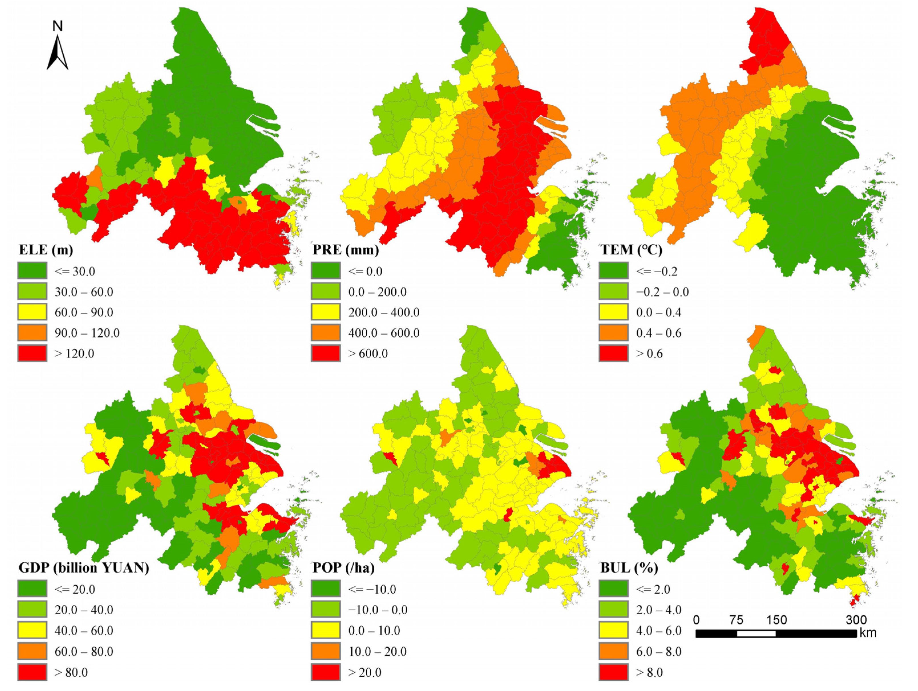
With consideration of natural and socioeconomic influences, six potential influencing factors were selected (Figure 3): elevation (ELE), changes in annual average precipitation (PRE), changes in annual average temperature (TEM), changes in GDP (GDP), changes in population density (POP), and changes in the proportion of built-up land (BUL).
Understanding how the influencing factors have contributed to the variations in the trade-offs/synergies among ESs is crucial for effective ecosystem management. Multiple linear regression (MLR) is one of the regression methods commonly used for exploring the relationships between multiple explanatory factors and independent variables [47,48]. Taking the study area as a whole, MLR can be used to explore the average regression coefficient by identifying a global relationship. The MLR used in this study is expressed in Equation (3):
where is the estimated TSD value; and represent the intercept and regression coefficients of independent variable , respectively; is the value of the independent variable at sample ; and ε is the random error term for sample .
A geographically weighted regression (GWR) model can estimate a location-specific regression coefficient for each unit in the study area by considering spatially varying relationships that exist between the dependent and independent variables. In this study, a GWR model was adopted to investigate the relationships between the related factors and the trade-offs/synergies while considering spatial heterogeneity. The formula used for the GWR is similar to that used for the MLR, except the former takes spatial heterogeneity into consideration. The GWR can be expressed as follows [49]:
where represents the TSD value for sample ; () represents the coordinates of sample ; is the constant term estimated for sample ; and is the estimated regression coefficient of factor at sample . represents the value of the independent variable that could explain TSD at sample ; is the random error term for sample . The regression coefficients of each sample are estimated by weighting all units around sample . The units closer to sample have a stronger impact on the estimated coefficient. The Gaussian kernel was selected to calculate the spatial weighting [50]:
where is the weight of sample for sample . represents the Euclidean distance between sample and sample . is the kernel bandwidth, which determines the range of spatial dependency. In this study, we selected the optimal bandwidth identified by the Akaike’s information criterion (AIC) method for the purposes of minimizing the AIC value: the estimated results with lower AIC values better reflect reality.
The performance of the regression models (MLR and GWR) can be measured and compared by considering R2 and AIC. R2 is the square of the correlation coefficient, indicating the degree of agreement between the estimated value and the observed value. AIC is not an absolute goodness of fit, but it can be used to effectively compare several different models. A difference between the AIC values of two models higher than 3 suggests that there is a significant difference between the two models. A more suitable model, which is assessed by its capability to better explain the variations in the dependent variables, tends to have a higher R2 and lower AIC.
3. Results
3.1. Spatial Patterns of ESs
As shown in Figure 4, forestland is mainly located in the southern part of the YRD region. High-intensity built-up land is concentrated along the Yangtze River. Cultivated land is mainly distributed in the northern part of the YRD region. As shown in Table 2, cultivated land accounted for 48.04% of the total area, the largest proportion of the YRD region, in 2015. Built-up land accounted for 11.90% of the total area in 2015.
From 2005 to 2015, built-up land increased by 5971.06 km2, which accounted for the largest proportion of change in land cover. In contrast, cultivated land, forestland, grassland and water bodies decreased. Cultivated land decreased significantly from 107,224.31 km2 to 101,105.46 km2 over ten years due to rapid urbanization. A large proportion of the decrease in cultivated land was caused by newly developed built-up land. Forestland and grassland decreased by 212.43 km2 and 195.63 km2 from 2005 to 2015, respectively.
Along with land cover changes in the YRD region, the selected ESs also varied over the study period. As shown in Table 3, the overall magnitude of CS, WP (measured by nitrogen export), and HQ in the YRD region decreased from 2005 to 2015. CS decreased marginally from 5.028 × 10⁸ to 5.014 × 10⁸ Mg. The total amount of WP decreased from 3.891 × 10⁷ kg to 3.794 × 10⁷ kg. The average value for HQ shows a declining trend, with the value decreasing from 0.385 in 2005 to 0.372 in 2015.
There is significant spatial heterogeneity in CS, WP, and HQ in 2005 and 2015. As shown in Figure 5, the high-provision areas for CS were mainly distributed in the southern mountainous area of the YRD, while the lower CS values were located in urban areas, where a large amount of non-built-up land had changed to built-up land. The high-provision areas for WP were mainly distributed in the northern area. WP in the YRD shows a gradual decreasing trend from southeast to northwest, which is consistent with the spatial patterns of the proportion of cultivated land. High values of HQ were found in the south areas, which are at higher elevations, while low value areas were mainly distributed in the north area. This result can be explained by the fact that areas with high elevations are mountainous with dense vegetation and rich biodiversity. In these areas, the natural environment, such as mountains, face fewer threats.
The majority of counties (157 out of 160 counties) in the YRD region show a decreasing trend in CS from 2005 to 2015 (Figure 6). Among these cities, Kunshan (Suzhou city) and Jiading (Shanghai city) experienced the most significant decline in average CS, decreasing by 17.831 Mg/ha and 15.236 Mg/ha, respectively. Dafeng, Xiaoshan, and Chongming showed a slight increase in average CS over the study period.
Overall, WP exhibited a downward trend across the YRD region. At the county level, over one-half (89) of the counties in the YRD region showed that WP is increasing, mainly in the eastern part of the YRD, accounting for 52.8% of the total area. Cultivated land was converted to BUL. The counties exhibiting a significant decrease in WP are in the southeastern part of the YRD, including Wenling, Yuhuan, and Huangyan.
Most of the counties (156) presented a declining trend for HQ, especially the Suzhou city core and Xiaoshan (Hangzhou city), decreasing by 33.3% and 18.3%, respectively. Only 4 counties experienced an increase from 2005–2015, mainly centralized in Nantong, Chuzhou, Yangzhou, and Taaizhou cities, accounting for 4.43% of the total area. The reduction in HQ was mainly due to significant urban expansion.
3.2. Spatiotemporal Dynamics of ESs Trade-Offs/Synergies
Spearman correlation analysis was employed to analyze the trade-off/synergy relationships between ES pairs. Both trade-offs and synergies were observed (Figure S1). We found that all three pairs of ESs (CS-WP, CS-HQ, WP-HQ) showed significant positive or negative correlations (p < 0.01). CS was significantly positively correlated with HQ. This result was supported by our findings that CS increased from 2005 to 2015, and HQ decreased over this period. The trade-offs between CS/HQ and WP/HQ suggested that a decrease or increase in one ES could lead to an increase or decrease in another ES in a specific county. CS had a strong and significant synergy with HQ, with a Spearman correlation coefficient larger than 0.7.
The TSD indicator was further applied to reveal the spatial distribution and magnitude of the trade-off/synergy relationships among the ESs. The TSD indicator is an extension of the traditional correlation analysis because it can detect local rather than global relationships between paired ESs. The relationships between paired ESs varied over space (Figure 7).
The negative TSD value for CS-WP were mainly distributed in the eastern and southwestern areas, which indicates that a decrease in CS could lead to an increase in WP in these regions. A larger amount of ecological land (forestland and grassland), the main type of land that supports CS, was occupied by built-up land due to the rapid development in this region. Significant urban expansion resulted in a decrease in CS. The loss in ecological land led to an increase in nitrogen export. Furthermore, the TSD values for CS-WP are lower in eastern and central regions and higher in southern and northwestern regions. The relationship between CS and WP is synergetic (TSD > 0) in the southeastern and northwestern areas, and this result contrasts with the implications of the Spearman correlation coefficient for CS-WP. This result suggests that a decrease in CS might decrease nitrogen export. This decrease may have occurred because cultivated land was converted to built-up land, and the increase in built-up land area might decrease CS. Additionally, built-up land produced less nitrogen loads than cultivated land.
CS and HQ mainly exhibited a synergistic relationship throughout the YRD region; this relationship can be attributed to high consistency in the land cover types of CS and HQ. For example, ecological land normally has higher values of CS and HQ. However, built-up land has a lower capacity for CS and HQ. The high TSD values for CS-HQ were mainly distributed in the eastern part of the YRD region, and the values gradually decreased from the eastern area to the western area of the YRD region. The Shanghai and Suzhou-Wuxi-Changzhou regions in the eastern area of the YRD region are the most developed areas and exhibit a significant increase in built-up land to meet increasing demand for socioeconomic development. Therefore, the trade-off intensity in this area is higher than in other areas.
Similar to the spatial distribution of the TSD value for CS-WP, a large proportion of counties exhibited trade-off relationships between WP and HQ in the eastern and southern areas of the YRD region, which means that the increase in nitrogen export might decrease HQ. In addition, the trade-off intensity gradually decreased from the eastern areas to the southern areas. This decrease may have occurred because newly cultivated land occupies a large amount of ecological land, which leads to a decrease in HQ and an increase in WP. Positive TSD values are observed in the northwestern and southeastern areas, which indicates that the relationship between WP and HQ is synergistic. Cultivated land was converted to built-up land due to the rapid socioeconomic development. Cultivated land performed worse in water purification because of its high proportion of agricultural land and frequent agricultural activities. Built-up land produced less nitrogen loads than cultivated land. Meanwhile, HQ decreased due to the increased proportion of built-up land.
The global Moran’s I for the TSD of each paired ES is presented in Table 4. The values of 0.8309, 0.3979, and 0.7216 for CS-WP, CS-HQ, and WP-HQ, respectively, suggest that the patterns of the trade-off/synergy relationships between the paired ESs were spatially autocorrelated.
3.3. The Impacts of Related Factors on the Trade-Offs/Synergies between ESs
We applied the MLR and GWR models to investigate the spatial relationships between the TSD and six natural and socioeconomic factors (ELE, PRE, TEM, GDP, POP, and BUL). In the study, VIF (variance inflation factor) was used to verify whether there is multicollinearity in the explanatory variables. If VIF exceeds 7.5, it means that the variable may be redundant. The results show that VIF values are all less than 7.5, which implies that only slight collinearity exists in the explanatory variables. The range of standardized residual values of the GWR model is −5.07–3.26, of which approximately 98.1% is −2.58–2.58. Therefore, the standardized residual values of the GWR model are randomly distributed with 95% confidence. As shown in Table 5, the R2 values of the GWR results are larger than those of the MLR model. The AIC values of the GWR are smaller than those of the MLR model. In contrast to the results of the MLR model, which is a global model for estimating the relationship between two variables, the GWR results provide a specific coefficient for each sample. The effects of the spatial relationship between the explanatory and dependent variables on the trade-offs/synergies between the ESs is explored.
Figure 8 presents the spatial distributions of the estimated regression coefficients of the influencing factors and trade-offs/synergies between paired ESs using the GWR model. The effects of the explanatory factors on ES trade-offs/synergies varied spatially. Both positive and negative coefficients are observed in the GWR results. A positive coefficient indicates that growth in the explanatory variable could increase the TSD value. In other words, the probability that the ES relationship will become more synergetic when the coefficient is positive. However, a negative coefficient suggests that a decrease in the dependent variables could decrease the probability that a synergistic relationship exists between the ESs, as evidenced by a declining TSD value.
Previous studies have highlighted elevation as one of the significant influencing factors affecting ecosystem services [39,51]. Elevation was positively correlated with the trade-off/synergy relationships between CS and WP in the eastern part of the YRD region. In contrast, a negative effect of elevation was mainly observed in the western area. It is found that the areas where a positive coefficient between elevation and TSD was present experienced a significant urban expansion, for example Shanghai, Suzhou, Nanjing. For a large area of the YRD region, there was a negative association between elevation and the CS-HQ relationship.
Vegetation is often influenced by climatic factors that affect their growth [52], which means that ESs are also influenced by the climatic factors. The direction and extent of the response of ESs to climatic factors normally present regional characteristics [53]. Precipitation is an important variable of the trade-off/synergy relationships from 2005–2015 (Figure 8). Changes in precipitation had a negative effect on CS-WP and WP-HQ. This result implies that an increase in precipitation may either increase the trade-off intensity or reduce the synergy intensity. The negative correlation between precipitation and the trade-off/synergy intensity for CS-HQ in the southern area was related to the relatively slow changes in CS and HQ.
The changes in TEM also had significant effects on the trade-off/synergy relationships between the paired ESs. Both positive and negative correlations between TEM and TSD were found across the YRD region. As presented in Figure 8, the spatial distributions of the coefficients for CS-WP and WP-HQ are similar. The change in TEM in the eastern and western areas exhibited a negative correlation with the trade-off/synergy intensity of CS-WP and WP-HQ. TEM had a positive effect on the TSD in the central and northern areas of the YRD region. As evidenced by Schuur (2003), the effects of climate factors on ESs are spatially heterogeneous [53].
As illustrated in Figure 8, GDP and POP have positive and negative correlations with the trade-offs/synergies between ESs. TSD values for CS-WP, CS-HQ, and WP-HQ have significant positive relationships with GDP and POP in the western area of the YRD region, where the intensity of human activity and the socioeconomic level are relatively weak compared with those in the eastern region. In the eastern area of the YRD region, however, an increase in GDP or POP will increase the probability that the relationships will convert to a trade-off.
The changes in built-up land are negatively correlated with CS-WP and WP-HQ relationships in the eastern area of the YRD region, where built-up land is concentrated and increased significantly over the study period (Figure 8). In addition, BUL exhibited a positive correlation with the synergy intensity of CS-HQ across the YRD region, and its effects gradually increased from southern areas to northern areas. This result implies that the synergy between CS and HQ is more sensitive to changes in BUL. CS and HQ are affected by a higher level of land-use consistency, and the increase in BUL could decrease the area of land cover types that support CS and HQ.
4. Discussion
4.1. Spatially Varying Trade-Offs/Synergies among the ESs and the Underlying Factors
By understanding the spatial patterns of the ES relationships’ responses to influencing factors, decision makers can regulate these factors to improve the synergy intensity and reduce unwanted trade-offs [44]. Our findings show that the trade-offs and synergies among multiple ESs (CS, WP, and HQ) were widespread in the YRD region, which is in accordance with the findings of previous studies [54,55]. However, studies concerning the spatial distribution of the intensity of trade-offs/synergies are scarce. Pairwise correlation coefficients are commonly used to reveal the global relationships between paired ESs [31,56]. This type of analysis reflects only the magnitude of a relationship and does not provide insight into the spatial patterns of a relationship. The hot spots of various ESs were compared to investigate the spatial relationship between two ESs. However, the results generated by hot spot comparisons do not indicate where trade-offs and synergies exist. The RMSE indicator was widely adopted in previous studies to measure the intensity of trade-offs for one temporal point [10,25], but changes in ESs over time are not considered in this indicator. Zhang et al. (2020) used a binary value (0, 1) to measure the relationship by comparing the changes in ESs between two points in time [29]. Although this type of analysis can identify the ES relationships, the magnitude of the relationships is not measured. Therefore, it is difficult to fully reveal the impact mechanisms of the trade-offs/synergies. In this study, we proposed a new indicator (TSD) to quantify the intensity of the trade-off/synergy relationships among ESs and their spatial heterogeneity rather than their spatial homogeneity. Compared with the findings of previous studies, our findings clarify the locations where trade-offs/synergies existed and their intensity.
Our study supports the argument that the relationships between ESs can be affected by natural and socioeconomic factors [57,58]. For appropriate ES management, decision makers should consider not only global correlations but also the spatial heterogeneity of the impacts to mitigate unwanted ES trade-offs. In contrast to the findings obtained by using correlation analysis and a global regression model [14,33], our results obtained by the GWR model can reveal the spatial relationship between trade-offs/synergies and the related factors. The intensity of trade-off/synergy relationships was significantly affected by natural factors and socioeconomic factors. A larger number of studies have confirmed that ESs are correlated with urbanization [59]. As indicated by the coefficient of determination (R2) from the GWR model, BUL had the largest effects on the relationships between paired ESs among these factors in the study. Su et al. (2014) argued that the effects of urbanization on Ess are spatially heterogeneous, with the magnitude of the effects varying spatially, which is similar to our findings [37]. However, previous studies considering topics related to the effects of influencing factors on the complex relationships that exist among multiple Ess were limited by the use of a global regression model and correlation analysis without considering spatial non-stationarity. In this study, goodness of fit tests employed to compare the MLR and GWR models were assessed using R2 and AIC. The results indicate that the GWR model has a strong explanatory capability for estimating the relationships between the influencing factors and the trade-off/synergy intensity of ESs. The coefficients estimated by the GWR model correspond to a specific geographic area, and the spatially varying effects of various factors can be explored through the creation of a spatial distribution map of the GWR coefficients.
A decrease in elevation could lead to an increase in synergy intensity of CS-HQ. This result may be related to the distribution of ecological land across different elevations. People prefer to live in lower terrain gradients, leading to a low ecosystem service values, and vice versa. When there is a decrease in elevation, the proportion of forest decreases and that of cultivated land and built-up land increases. The urban expansion rate in this area is relatively higher than that in areas in higher elevations. The decreases in CS and HQ are relatively significant; thus, TSD value was enhanced. In the YRD region, the vegetation coverage area increased as precipitation increased, CS and HQ were enhanced, and WP decreased; thus, trade-off intensities of CS-WP and WP-HQ increased. Additionally, the effects of precipitation in the southern area of the YRD region are greater than those in other areas due to its higher proportion of ecological land and significantly higher levels of precipitation. With increases in GDP and population, socio-economic dependent land continuously occupied ecological land, and waste gas and water put added pressure on regulating and supporting services of the ecosystem. The newly expanded built-up land occupied a larger amount of cultivated and ecological land, which led to a significant decline in CS and HQ because of the loss of land cover classes that support CS and HQ. In contrast, urbanization was positively correlated with nitrogen export due to heavy pollutant loads on impervious surfaces and the weak purification ability of the limited amount of vegetation coverage.
4.2. Policy Implications
Integrating information about the trade-offs/synergies between ESs into ecological planning and management is a prerequisite for coordinating the relationship between ecological protection and socioeconomic development [60]. This study quantitatively explores the influencing mechanisms of natural and socioeconomic processes on the trade-off/synergy relationships among ESs, which is helpful for developing scientific and effective ecosystem service management practices and regional planning. Recommendations for ES regulation and promotion that correspond to our results are as follows:
First, in the context of the collaborative development of the YRD region, it is crucial to enhance the implementation of precisely targeted ecological projects and refine ecological management policies based on the analysis of the trade-offs/synergies among ESs. In recent years, a range of ecological projects have been carried out, such as the Grain for Green Project, the Natural Forest Protection Project, and Reclaiming Lake from Farmland [61]. These ecological projects play a key role in enhancing the ecological functions of regional water conservation and soil and water conservation and accelerating the construction of a green ecological corridor in the YRD region. However, ES degradation was still observed in some ecologically sensitive and rapidly developed areas. The YRD region still faces a great challenge in achieving the ‘win-win’ goal of socioeconomic development and ecological protection. Reaching this goal may be difficult because the trade-off/synergy relationships and their spatial heterogeneity, and impact factors have been neglected in ecological projects. Therefore, it is important to integrate the complex interactions among ESs into the design and implementation of various ecological projects to promote the efficiency of ecological protection and restoration.
Second, our findings reveal the specific regions where trade-off/synergy relationships exist, which is helpful information for decision making regarding trade-offs in specific locations and implementing ES management more effectively. The YRD region can be separated into three areas based on the intensity of land development, population concentration and changes in ESs: optimized development area, key development area and restricted development area. Different development strategies should be developed for various areas. The optimized development area refers to the area where the carrying capacity of resources and the environment is saturated. This area is mainly distributed in Shanghai, Hangzhou, and southern Jiangsu. We should take effective measures to strictly control the scale and intensity of new construction land and appropriately expand agricultural and ecological spaces. The key development area refers to the area with great potential for the carrying capacity of resources and the environment. This area is mainly distributed in central Jiangsu, central Zhejiang, central Anhui and the coastal area. It is necessary to strengthen the capacity of industrial and population agglomeration, appropriately expand industrial and urban spaces, optimize the rural living space, and strictly protect the green ecological space. The restricted development area refers to the area with significant ecological sensitivity and a low carrying capacity of resources and the environment. This area is mainly distributed in northern Jiangsu, western Anhui and western Zhejiang. It is necessary to strictly control the scale of new construction land; promote the concentrated development of cities; strengthen the protection of water resources, ecological restoration and construction; and maintain the stability of the ecosystem structure and its functioning.
Third, the land development intensity in the YRD region was 17.1% in 2013, which was 15% higher than that due to Japan’s Pacific coastal urban agglomeration, and the potential space available for subsequent construction is insufficient. Shanghai’s development intensity is as high as 36%, far more than that of Paris at 21% and that of London at 24%. Due to extensive and unrestrained development, new development zones and industrial parks occupy too much land, which seriously affects the overall ecosystem structure and utilization efficiency of regional land space [62]. Therefore, the “three red lines” (Ecological Protection Red Line, Cultivated land Protection Red Line, and Urban Development Boundary Red Line) policy for spatial planning was proposed to improve land-use efficiency [63]. Despite the common acknowledgements of the importance of the three red lines in sustainable development, there are several issues that need to be addressed, including the lack of consideration of the trade-off relationships that exist among ESs, when identifying the three red lines. The establishment of the three red lines could lead to an ES trade-off, where one ES is promoted at the expense of other ESs.
4.3. Limitations and Further Study
Although this study obtained some interesting findings, some limitations exist. Firstly, the TSD indicator was developed and applied to analyze the trade-offs/synergies among ESs in the YRD region and effectively quantify the complex relationships that exist between ESs. However, a temporal scale was not included in this study. Some scholars have pointed out that the relationship between ESs varies temporally [19,21]. In addition, the reliability of the results regarding the trade-offs/synergies can be improved by using long-term time series data. Therefore, future studies need to identify the relationships between ESs using long-term series data to mitigate uncertainty about the trade-offs/synergies that exist among ESs and analyze the impacts at the temporal scale. Secondly, the TSD indicator did not consider the spatial dependence of ESs. As some studies suggested that the supply of ESs in any given location depends upon juxtaposition with other ESs and on the overall mosaic of ESs across a region [64,65]. It is therefore, crucial to consider spatial dependence of ESs in future studies. Thirdly, limitations exist in terms of the analysis of the influence mechanisms of the trade-offs/synergies among ESs. This study investigated the effects of natural and socioeconomic factors on the trade-off/synergy relationships among ESs by considering six factors (ELE, PRE, TEM, GDP, POP, BUL). The findings suggest that these factors have significant effects on ES relationships. However, the complex relationships between ESs may be affected by other factors (e.g., soil properties, slope, solar radiation) [66,67]. It is of great importance to consider more potential factors to improve the understanding of the influence mechanisms of the trade-offs/synergies that exist among ESs. Finally, it is widely acknowledged that a better understanding of the relationships between ES supply and demand is important for sustainable ES management and the improvement of human wellbeing. However, the study analyzed the trade-off/synergy relationships from the perspective of ES supply. Therefore, the supply-demand relationships should be involved in future studies. The results of such an analysis will provide a more scientific support for sustainable development.
5. Conclusions
The results of the trade-off/synergy analysis enable decision makers to develop effective regional planning and ecological management policies that promote sustainable development. In this study, we investigated spatiotemporal changes in three ESs, namely, CS, WP, and HQ, in the YRD region from 2005 to 2015. The results revealed that CS, WP, and HQ decreased by 0.28%, 2.49%, and 3.38%, respectively. These variations in three key ESs in the YRD region imply that ESs have degraded mainly due to intensive human disturbance in recent years. In addition to measuring the trade-off/synergy relationships between multiple ESs, this study measured their magnitude using an innovative indicator (TSD). The TSD indicator was proven to be efficient for identifying the types of relationships that exist between ESs and quantifying the intensity of the trade-offs/synergies. The relationships between the factors and trade-offs/synergies were revealed by using MLR and GWR models. This study demonstrated that the trade-off/synergy relationships presented significant autocorrelations. The GWR model performed better than the MLR model in explaining variations in the trade-off/synergy intensity, as the GWR model generated higher R2 values and lower AIC values. The impacts of natural and socioeconomic factors on the trade-offs/synergies were spatially heterogeneous rather than spatially consistent. Our findings show that the GWR model can be used to obtain precise information on the various roles of the related factors at different sites in the study area rather than producing a global coefficient for the entire area. The trade-off/synergy intensity is significantly correlated with meteorological, urbanization, and terrain factors. The findings improve the understanding of the trade-off/synergy relationships that exist among ESs and their influencing mechanisms. The trade-off/synergy relationships among ESs in the YRD region are not only affected by environmental factors but also significantly related to socioeconomic development. Furthermore, the spatial heterogeneity of the trade-offs/synergies is well explained by the influencing factors. The GWR model revealed that these relationships are spatially heterogeneous rather than spatially consistent relationships.
Supplementary Materials
The following are available online at https://0-www-mdpi-com.brum.beds.ac.uk/article/10.3390/land11010106/s1, Figure S1: Coefficients of the Spearman correlations between paired ESs (** p < 0.01), Table S1: Carbon density per unit area of different land cover types in the YRD region, China (Unit: Mg/ha), Table S2: Biophysical table in water purification module for the YRD region, China, Table S3: Parameters for habitat quality in the YRD region, China.
Author Contributions
Conceptualization, C.L.; methodology, J.Z.; validation, J.Z.; writing—original draft preparation, J.Z.; writing—review and editing, C.L. All authors have read and agreed to the published version of the manuscript.
Funding
This research was funded by the National Natural Science Foundation of China, grant number 41801197, 42001241 and the Project of Philosophy and Social Science Research in Colleges and Universities in Jiangsu Province, grant number 2020SJA1006.
Institutional Review Board Statement
Not applicable.
Informed Consent Statement
Not applicable.
Data Availability Statement
Land cover data on the study area for 2005 and 2015 were obtained from the Data Centre for Resources and Environmental Sciences, Chinese Academy of Sciences (RESDC). http://www.resdc.cn/Default.aspx (accessed on 7 December 2021); Meteorological data, including information on precipitation, total solar radiation and the temperature in the YRD region from 2005 to 2015, were derived from the China Meteorological Data Service Centre. http://data.cma.cn/ (accessed on 7 December 2021); Soil property data, including soil depth and the content percentage of sand, clay, silt and organic matter at the scale of 1:1,000,000, were obtained from the Harmonized World Soil Database version 1.1 (HWSD) http://data.tpdc.ac.cn/zh-hans/ (accessed on 7 December 2021); Digital elevation model (DEM) data for the YRD region with a resolution of 30 m were obtained from the Geospatial Data Cloud http://www.gscloud.cn/ (accessed on 7 December 2021); Normalized Difference Vegetation Index (NDVI) data for the YRD region with a resolution of 1 km were obtained from the Data Centre for Resources and Environmental Sciences, Chinese Academy of Sciences (RESDC) http://www.resdc.cn/Default.aspx (accessed on 7 December 2021).
Conflicts of Interest
The authors declare no conflict of interest. The funders had no role in the design of the study; in the collection, analyses, or interpretation of data; in the writing of the manuscript, or in the decision to publish the results.
References
- MEA (Millennium Ecosystem Assessment). Ecosystems and Human Well-Being; Island Press: Washington, DC, USA, 2005. [Google Scholar]
- Zhou, D.; Tian, Y.; Jiang, G. Spatio-temporal investigation of the interactive relationship between urbanization and ecosystem services: Case study of the Jingjinji urban agglomeration, China. Ecol. Indic. 2018, 95, 152–164. [Google Scholar] [CrossRef]
- Haase, D.; Schwarz, N.; Strohbach, M.; Kroll, F.; Seppelt, R. Synergies, trade-offs, and losses of ecosystem services in urban regions: An integrated multiscale framework applied to the Leipzig-Halle region, Germany. Ecol. Soc. 2012, 17, 22. [Google Scholar] [CrossRef]
- Feng, Q.; Zhao, W.; Fu, B.; Ding, J.; Wang, S. Ecosystem service trade-offs and their influencing factors: A case study in the Loess Plateau of China. Sci. Total Environ. 2017, 607–608, 1250–1263. [Google Scholar] [CrossRef]
- Christensen, N.L.; Bartuska, A.M.; Brown, J.H.; Carpenter, S.; D’Antonio, C.; Francis, R.; Franklin, J.F.; MacMahon, J.A.; Noss, R.F.; Parsons, D.J.; et al. The report of the ecological society of America committee on the scientific basis for ecosystem management. Ecol. Appl. 1996, 6, 665–691. [Google Scholar] [CrossRef] [Green Version]
- Groot, J.C.J.; Yalew, S.G.; Rossing, W.A.H. Exploring ecosystem services trade-offs in agricultural landscapes with a multi-objective programming approach. Landsc. Urban Plan. 2018, 172, 29–36. [Google Scholar] [CrossRef]
- Sherrouse, B.C.; Semmens, D.J.; Ancona, Z.H.; Brunner, N.M. Analyzing land-use change scenarios for trade-offs among cultural ecosystem services in the Southern Rocky Mountains. Ecosyst. Serv. 2017, 26, 431–444. [Google Scholar] [CrossRef]
- Xu, X.; Yang, G.; Tan, Y.; Liu, J.; Hu, H. Ecosystem services trade-offs and determinants in China’s Yangtze River Economic Belt from 2000 to 2015. Sci. Total Environ. 2018, 634, 1601–1614. [Google Scholar] [CrossRef]
- Zheng, H.; Li, Y.; Robinson, B.E.; Liu, G.; Ma, D.; Wang, F.; Lu, F.; Ouyang, Z.; Daily, G.C. Using ecosystem service trade-offs to inform water conservation policies and management practices. Front. Ecol. Environ. 2016, 14, 527–532. [Google Scholar] [CrossRef]
- Lauf, S.; Haase, D.; Kleinschmit, B. Linkages between ecosystem services provisioning, urban growth and shrinkage-A modeling approach assessing ecosystem service trade-offs. Ecol. Indic. 2014, 42, 73–94. [Google Scholar] [CrossRef]
- Darvill, R.; Lindo, Z. The inclusion of stakeholders and cultural ecosystem services in land management trade-off decisions using an ecosystem services approach. Landsc. Ecol. 2016, 31, 533–545. [Google Scholar] [CrossRef]
- Langner, A.; Irauschek, F.; Perez, S.; Pardos, M.; Zlatanov, T.; Öhman, K.; Nordström, E.-M.; Lexer, M.J. Value-based ecosystem service trade-offs in multi-objective management in European mountain forests. Ecosyst. Serv. 2017, 26, 245–257. [Google Scholar] [CrossRef]
- Landuyt, D.; Broekx, S.; Goethals, P.L.M. Bayesian belief networks to analyse trade-offs among ecosystem services at the regional scale. Ecol. Indic. 2016, 71, 327–335. [Google Scholar] [CrossRef]
- Feng, Q.; Zhao, W.; Hu, X.; Liu, Y.; Daryanto, S.; Cherubini, F. Trading-off ecosystem services for better ecological restoration: A case study in the Loess Plateau of China. J. Clean. Prod. 2020, 257, 120469. [Google Scholar] [CrossRef]
- Goldstein, J.H.; Caldarone, G.; Duarte, T.K.; Ennaanay, D.; Hannahs, N.; Mendoza, G.; Polasky, S.; Wolny, S.; Daily, G.C. Integrating ecosystem-service tradeoffs into land-use decisions. Proc. Natl. Acad. Sci. USA 2012, 109, 7565–7570. [Google Scholar] [CrossRef] [PubMed] [Green Version]
- Baró, F.; Gómez-Baggethun, E.; Haase, D. Ecosystem service bundles along the urban-rural gradient: Insights for landscape planning and management. Ecosyst. Serv. 2017, 24, 147–159. [Google Scholar] [CrossRef] [Green Version]
- Washbourne, C.-L.; Goddard, M.A.; Provost, G.L.; Manning, D.A.C.; Manning, P. Trade-offs and synergies in the ecosystem service demand of urban brownfield stakeholders. Ecosyst. Serv. 2020, 42, 101074. [Google Scholar] [CrossRef]
- Zhou, Z.X.; Li, J.; Guo, Z.Z.; Li, T. Trade-offs between carbon, water, soil and food in Guanzhong-Tianshui economic region from remotely sensed data. Int. J. Appl. Earth Obs. Geoinf. 2017, 58, 145–156. [Google Scholar] [CrossRef]
- Wu, Y.; Tao, Y.; Yang, G.; Ou, W.; Pueppke, S.; Sun, X.; Chen, G.; Tao, Q. Impact of land use change on multiple ecosystem services in rapidly urbanization Kunshan City of China: Past trajectories and future projections. Land Use Policy 2019, 85, 419–427. [Google Scholar] [CrossRef]
- Asadolahi, Z.; Salmanmahiny, A.; Sakieh, Y.; Mirkarimi, S.H.; Baral, H.; Azimi, M. Dynamic trade-off analysis of multiple ecosystem services under land use change scenarios: Towards putting ecosystem services into planning in Iran. Ecol. Complex. 2018, 36, 250–260. [Google Scholar] [CrossRef]
- Braun, D.; Damm, A.; Hein, L.; Petchey, O.L.; Schaepman, M.E. Spatio-temporal trends and trade-offs in ecosystem services: An Earth observation based assessment for Switzerland between 2004 and 2014. Ecol. Indic. 2018, 89, 828–839. [Google Scholar] [CrossRef]
- Kubiszewski, I.; Costanza, R.; Anderson, S.; Sutton, P. The future value of ecosystem services: Global scenarios and national implications. Ecosyst. Serv. 2017, 26, 289–301. [Google Scholar] [CrossRef]
- Bennett, E.M.; Peterson, G.D.; Gordon, L.J. Understanding relationships among multiple ecosystem services. Ecol. Lett. 2019, 12, 1394–1404. [Google Scholar] [CrossRef]
- Castro, A.J.; Verburg, P.H.; Martín-López, B.; Garcia-Llorente, M.; Cabello, J.; Vaughn, C.C.; López, E. Ecosystem service trade-offs from supply to social demand: A landscape-scale spatial analysis. Landsc. Urban Plan. 2014, 132, 102–110. [Google Scholar] [CrossRef]
- Laterra, P.; Orue, M.E.; Booman, G.C. Spatial complexity and ecosystem services in rural landscape. Agric. Ecosyst. Environ. 2012, 154, 56–67. [Google Scholar] [CrossRef]
- Bradford, J.B.; D’Amato, A.W. Recognizing trade-offs in multi-objective land management. Front. Ecol. Environ. 2012, 10, 210–216. [Google Scholar] [CrossRef] [Green Version]
- Pan, Y.; Xu, Z.; Wu, J. Spatial differences of the supply of multiple ecosystem services and the environmental and land use factors affecting them. Ecosyst. Serv. 2013, 5, 4–10. [Google Scholar] [CrossRef]
- Locatelli, B.; Imbach, P.; Wunder, S. Synergies and trade-offs between ecosystem services in Costa Rica. Environ. Conserv. 2014, 41, 27–36. [Google Scholar] [CrossRef] [Green Version]
- Zhang, Z.; Liu, Y.; Wang, Y.; Liu, Y.; Zhang, Y.; Zhang, Y. What factors affect the synergy and tradeoff between ecosystem services, and how, from a geospatial perspective? J. Clean. Prod. 2020, 257, 120454. [Google Scholar] [CrossRef]
- Dade, M.C.; Mitchell, M.G.E.; McAlpine, C.A.; Rhodes, J.R. Assessing ecosystem service trade-offs and synergies: The need for a more mechanistic approach. Ambio 2018, 48, 1116–1128. [Google Scholar] [CrossRef]
- Ndong, G.O.; Villerd, J.; Cousin, I.; Therond, O. Using a multivariate regression tree to analyze trade-offs between ecosystem services: Application to the main cropping area in France. Sci. Total Environ. 2020, 764, 142815. [Google Scholar] [CrossRef]
- He, J.; Shi, X.; Fu, Y.; Yuan, Y. Evaluation and simulation of the impact of land use change on ecosystem services trade-offs in ecological restoration areas, China. Land Use Policy 2020, 99, 105020. [Google Scholar] [CrossRef]
- Zhong, L.; Wang, J.; Zhang, X.; Ying, L. Effects of agricultural land consolidation on ecosystem services: Trade-offs and synergies. J. Clean. Prod. 2020, 264, 121412. [Google Scholar] [CrossRef]
- Chisholm, R.A. Trade-offs between ecosystem services: Water and carbon in a biodiversity hotspot. Ecol. Econ. 2010, 69, 1973–1987. [Google Scholar] [CrossRef]
- Bai, Y.; Zheng, H.; Ouyang, Z.; Zhuang, C.; Jiang, B. Modeling hydrological ecosystem services and tradeoffs: A case study in Baiyangdian watershed, China. Environ. Earth Sci. 2013, 70, 709–718. [Google Scholar] [CrossRef]
- Fotheringham, A.S.; Brunsdon, C. Local forms of spatial analysis. Geogr. Anal. 1999, 31, 340–358. [Google Scholar] [CrossRef]
- Su, S.; Li, D.; Hu, Y.; Xiao, R.; Zhang, Y. Spatially non-stationary response of ecosystem service value changes to urbanization in Shanghai, China. Ecol. Indic. 2014, 45, 332–339. [Google Scholar] [CrossRef]
- Foody, G.M. Geographical weighting as a further refinement to regression modelling: An example focused on the NDVI–rainfall relationship. Remote Sens. Environ. 2003, 88, 283–293. [Google Scholar] [CrossRef]
- Wang, S.; Liu, Z.; Chen, Y.; Fang, C. Factors influencing ecosystem services in the Pearl River Delta, China: Spatiotemporal differentiation and varying importance. Resour. Conserv. Recycl. 2021, 168, 105477. [Google Scholar] [CrossRef]
- Haines-Young, R.; Potschin, M. The Links between Biodiversity, Ecosystem Services and Human Well-Being. In Ecosystem Ecology: A New Synthesis; Raffaelli, D., Frid, C., Eds.; Cambridge University Press: Cambridge, UK, 2010; pp. 110–139. [Google Scholar] [CrossRef]
- Cook, D.; Davíðsdóttir, B.; Malinauskaite, L. A cascade model and initial exploration of co-production processes underpinning the ecosystem services of geothermal areas. Renew. Energy 2020, 161, 917–927. [Google Scholar] [CrossRef]
- Zhang, Y.; Liu, Y.; Zhang, Y.; Liu, Y.; Zhang, G.; Chen, Y. On the spatial relationship between ecosystem services and urbanization: A case study in Wuhan, China. Sci. Total Environ. 2018, 637–638, 780–790. [Google Scholar] [CrossRef] [PubMed]
- Chuai, X.; Huang, X.; Lai, L.; Wang, W.; Peng, J.; Zhao, R. Land use structure optimization based on carbon storage in several regional terrestrial ecosystems across China. Environ. Sci. Policy 2013, 25, 50–61. [Google Scholar] [CrossRef]
- Cord, A.F.; Bartkowski, B.; Beckmann, M.; Dittrich, A.; Hermans-Neumann, K.; Kaim, A.; Lienhoop, N.; Locher-Krause, K.; Priess, J.; Schröter-Schlaack, C.; et al. Towards systematic analyses of ecosystem service trade-offs and synergies: Main concepts, methods and the road ahead. Ecosyst. Serv. 2017, 28, 264–272. [Google Scholar] [CrossRef]
- Wu, J.S.; Feng, Z.; Gao, Y.; Peng, J. Hotspot and relationship identification in multiple landscape services: A case study on an area with intensive human activities. Ecol. Indic. 2013, 29, 529–537. [Google Scholar] [CrossRef]
- Anselin, L. Local indicators of spatial association-LISA. Geogr. Anal. 1995, 27, 93–115. [Google Scholar] [CrossRef]
- Chagas, C.D.S.; Junior, W.D.C.; Bhering, S.B.; Filho, B.C. Spatial prediction of soil surface texture in a semiarid region using random forest and multiple linear regressions. Catena 2016, 139, 232–240. [Google Scholar] [CrossRef]
- Yu, H.; Gong, H.; Chen, B.; Liu, K.; Gao, M. Analysis of the influence of groundwater on land subsidence in Beijing based on the geographical weighted regression (GWR) model. Sci. Total Environ. 2020, 738, 139405. [Google Scholar] [CrossRef]
- Fotheringham, A.S.; Charlton, M.; Brunsdon, C. Measuring Spatial Variations in Relationships with Geographically Weighted Regression. In Recent Developments in Spatial Analysis; Fischer, M.M., Getis, A., Eds.; Springer: Berlin/Heidelberg, Germany, 1997; pp. 60–82. [Google Scholar]
- Fotheringham, A.S.; Charlton, M.E.; Brunsdon, C. Geographically weighted regression: A natural evolution of the expansion method for spatial data analysis. Environ. Plan. A Econ. Space 1998, 30, 1905–1927. [Google Scholar] [CrossRef]
- Zhu, M.; He, W.; Zhang, Q.; Xiong, Y.; Tan, S.; He, H. Spatial and temporal characteristics of soil conservation service in the area of the upper and middle of the Yellow River, China. Heliyon 2019, 5, e02985. [Google Scholar] [CrossRef] [Green Version]
- Bangash, R.F.; Passuello, A.; Sanchez-Canales, M.; Terrado, M.; Lopez, A.; Elorza, F.J.; Ziv, G.; Acuna, V.; Schuhmacher, M. Ecosystem services in Mediterranean river basin: Climate change impact on water provisioning and erosion control. Sci. Total Environ. 2013, 458–460, 246–255. [Google Scholar] [CrossRef]
- Schuur, E.A.G. Productivity and global climate revisited: The sensitivity of tropical forest growth to precipitation. Ecology 2003, 84, 1165–1170. [Google Scholar] [CrossRef]
- Bai, Y.; Chen, Y.; Alatalo, J.M.; Yang, Z.; Jiang, B. Scale effects on the relationships between land characteristics and ecosystem services- a case study in Taihu Lake Basin, China. Sci. Total Environ. 2020, 716, 137083. [Google Scholar] [CrossRef]
- Jopke, C.; Kreyling, J.; Maes, J.; Koellner, T. Interactions among ecosystem services across Europe: Bagplots and cumulative correlation coefficients reveal synergies, trade-offs, and regional patterns. Ecol. Indic. 2015, 49, 46–52. [Google Scholar] [CrossRef]
- Morán-Ordóñez, A.; Ameztegui, A.; De Cáceres, M.; de-Miguel, S.; Lefèvre, F.; Brotons, L.; Coll, L. Future trade-offs and synergies among ecosystem services in Mediterranean forests under global change scenarios. Ecosyst. Serv. 2020, 45, 101174. [Google Scholar] [CrossRef]
- Dennis, M.; James, P. Considerations in the valuation of urban green space: Accounting for user participation. Ecosyst. Serv. 2016, 21, 120–129. [Google Scholar] [CrossRef]
- Syrbe, R.U.; Walz, U. Spatial indicators for the assessment of ecosystem services: Providing, benefiting and connecting areas and landscape metrics. Ecol. Indic. 2012, 21, 80–88. [Google Scholar] [CrossRef]
- Baró, F.; Palomo, I.; Zulian, G.; Vizcaino, P.; Haase, D.; Gomez-Baggethun, E. Mapping ecosystem service capacity, flow and demand for landscape and urban planning: A case study in the Barcelona metropolitan region. Land Use Policy 2016, 57, 405–417. [Google Scholar] [CrossRef] [Green Version]
- Peng, J.; Hu, X.; Zhao, M.; Liu, Y. Research progress on ecosystem service trade- offs: From cognition to decision-making. Acta Geogr. Sin. 2017, 72, 960–973. [Google Scholar] [CrossRef]
- Gao, J.; Yu, Z.; Wang, L.; Vejre, H. Suitability of regional development based on ecosystem service benefits and losses: A case study of the Yangtze River Delta urban agglomeration, China. Ecol. Indic. 2019, 107, 105579. [Google Scholar] [CrossRef]
- Xu, F.; Wang, Z.; Chi, G.; Zhang, Z. The impacts of population and agglomeration development on land use intensity: New evidence behind urbanization in China. Land Use Policy 2020, 95, 104639. [Google Scholar] [CrossRef]
- He, P.; Gao, J.; Zhang, W.; Rao, S.; Zou, C.; Du, J.; Liu, W. China integrating conservation areas into red lines for stricter and unified management. Land Use Policy 2018, 71, 245–248. [Google Scholar] [CrossRef]
- Li, J.; Convertino, M. Inferring ecosystem networks as information flows. Sci. Rep. 2021, 11, 7094. [Google Scholar] [CrossRef]
- Lamy, T.; Liss, K.N.; Gonzalez, A.; Bennett, E.M. Landscape structure affects the provision of multiple ecosystem services. Environ. Res. Lett. 2016, 11, 124017. [Google Scholar] [CrossRef]
- Sun, X.; Shan, R.; Liu, F. Spatio-temporal quantification of patterns, trade-offs and synergies among multiple hydrological ecosystem services in different topographic basins. J. Clean. Prod. 2020, 268, 122338. [Google Scholar] [CrossRef]
- Schirpke, U.; Candiago, S.; Vigl, L.E.; Jäger, H.; Labadini, A.; Marsoner, T.; Meisch, C.; Tasser, E.; Tappeiner, U. Integrating supply, flow and demand to enhance the understanding of interactions among multiple ecosystem services. Sci. Total Environ. 2019, 651, 928–941. [Google Scholar] [CrossRef]
Figure 1.
The YRD.

Figure 2.
Ecosystem services cascade model.

Figure 3.
The spatial distribution of potential influencing factors (ELE: elevation, PRE: changes in annual average precipitation, TEM: changes in annual average temperature, GDP: changes in gross domestic product, POP: changes in population density, BUL: changes in the proportion of built-up land).

Figure 4.
Land cover map of the YRD region in 2005 and 2015.

Figure 5.
Spatial patterns of ESs in the YRD region at the grid scale (CS: carbon storage; WP: water purification; HQ: habitat quality).
Figure 5.
Spatial patterns of ESs in the YRD region at the grid scale (CS: carbon storage; WP: water purification; HQ: habitat quality).

Figure 6.
Spatial patterns of ES variations at the county scale in the YRD region (CS: carbon storage; WP: water purification; HQ: habitat quality. 1: Kunshan; 2: Jiading; 3: Dafeng; 4: Xiaoshan; 5: Chongming; 6: Wenling; 7: Yuhuan; 8: Huangyan).
Figure 6.
Spatial patterns of ES variations at the county scale in the YRD region (CS: carbon storage; WP: water purification; HQ: habitat quality. 1: Kunshan; 2: Jiading; 3: Dafeng; 4: Xiaoshan; 5: Chongming; 6: Wenling; 7: Yuhuan; 8: Huangyan).

Figure 7.
Spatial patterns of the synergies and trade-offs (measured by TSD) among multiple ESs at the county scale in the YRD region (CS: carbon storage; WP: water purification; HQ: habitat quality).
Figure 7.
Spatial patterns of the synergies and trade-offs (measured by TSD) among multiple ESs at the county scale in the YRD region (CS: carbon storage; WP: water purification; HQ: habitat quality).

Figure 8.
Coefficients of the relationship between the TSD of paired ESs and six variables using the GWR model.
Figure 8.
Coefficients of the relationship between the TSD of paired ESs and six variables using the GWR model.


Table 1.
Methods and calculations used to estimate the ESs.
| ES | Method | Formula and Variable Description |
|---|---|---|
| Carbon Storage (CS) | InVEST carbon storage and sequestration model | : above ground biomass carbon stocks; : below ground biomass carbon stocks; : soil carbon stocks; : dead organic matter carbon stocks. The biomass carbon density for the different land-use types was derived from the results of a relevant study [43] (Table S1) |
| Water Purification (WP) | InVEST nutrient delivery model | : sum of the water yield of grid cell along the flow path above grid cell x. The biophysical parameters for water purification was presented in Table S2. |
| Habitat Quality (HQ) | InVEST HQ model | if linear if exponential : maximum effective distance of the threat. The parameters used in the model were presented in Table S3. HQ is a measure of the quality of the ecological infrastructure. |
Table 2.
Area of various land cover types in the YRD region in 2005 and 2015 (km2).
| Cultivated Land | Forestland | Grassland | Wetland | Built-Up Land | Unused Land | |
|---|---|---|---|---|---|---|
| 2005 | 107,224.31 50.94 | 57,424 | 7377.18 | 19,340.63 | 19,072.64 | 34.16 |
| Proportion (%) | 27.28 | 3.51 | 9.19 | 9.06 | 0.02 | |
| 2015 | 101,105.46 48.04 | 57,211.60 | 7181.55 | 19,721.11 | 25,043.70 | 209.53 |
| Proportion (%) | 27.18 | 3.41 | 9.37 | 11.90 | 0.10 | |
| 2005–2015 | −6118.85 | −212.43 | −195.63 | 380.48 | 5971.03 | 175.37 |
Table 3.
The total amount of ESs in the YRD region in 2005 and 2015.
| Title 1 | CS (Mg) | WP (kg) | HQ |
|---|---|---|---|
| 2005 | 5.028 × 10⁸ | 3.891 × 10⁷ | 0.385 |
| 2015 | 5.014 × 10⁸ | 3.794 × 10⁷ | 0.372 |
| 2005–2015 | −0.28% | −2.49% | −3.38% |
Table 4.
Global Moran’s I of the TSD values between paired ESs.
| Pairs of ESs | Moran’s I | z-Score | p-Value |
|---|---|---|---|
| CS-WP | 0.8309 | 11.5593 | 0.0000 |
| CS-HQ | 0.3979 | 5.6219 | 0.0000 |
| WP-HQ | 0.7216 | 10.0640 | 0.0000 |
Table 5.
R2 and AIC values for the GWR and MLR models.
| Factors | Indicator | CS-WP | CS-HQ | WP-HQ | |||
|---|---|---|---|---|---|---|---|
| MLR | GWR | MLR | GWR | MLR | GWR | ||
| ELE | R2 | 0.0137 | 0.8031 | 0.0981 | 0.3950 | 0.0213 | 0.7643 |
| AIC | 29.9511 | −148.1661 | −55.1897 | −77.0673 | −4.8324 | −165.4915 | |
| PRE | R2 | 0.5777 | 0.7456 | 0.0071 | 0.3093 | 0.6076 | 0.7444 |
| AIC | −105.7788 | −163.5704 | −39.8081 | −74.5886 | −151.0859 | −197.8709 | |
| TEM | R2 | 0.0279 | 0.7900 | 0.0063 | 0.2966 | 0.0420 | 0.7538 |
| AIC | 27.6261 | −162.3956 | −39.6942 | −75.4645 | −8.2591 | −187.0395 | |
| GDP | R2 | 0.0659 | 0.7732 | 0.0713 | 0.3445 | 0.0583 | 0.7658 |
| AIC | 21.2469 | −140.3177 | −50.5173 | −79.4526 | −10.9957 | −168.7866 | |
| POP | R2 | 0.0255 | 0.7697 | 0.0744 | 0.3252 | 0.0098 | 0.7538 |
| AIC | 28.0298 | −132.7592 | −51.0407 | −74.8401 | −2.9728 | −155.6341 | |
| BUL | R2 | 0.1786 | 0.8640 | 0.7864 | 0.8055 | 0.1597 | 0.8170 |
| AIC | 0.6776 | −203.8839 | −285.6687 | −290.4239 | −29.2331 | −193.8583 | |
Publisher’s Note: MDPI stays neutral with regard to jurisdictional claims in published maps and institutional affiliations. |
© 2022 by the authors. Licensee MDPI, Basel, Switzerland. This article is an open access article distributed under the terms and conditions of the Creative Commons Attribution (CC BY) license (https://creativecommons.org/licenses/by/4.0/).
Share and Cite
MDPI and ACS Style
Zhao, J.; Li, C. Investigating Ecosystem Service Trade-Offs/Synergies and Their Influencing Factors in the Yangtze River Delta Region, China. Land 2022, 11, 106. https://0-doi-org.brum.beds.ac.uk/10.3390/land11010106
AMA Style
Zhao J, Li C. Investigating Ecosystem Service Trade-Offs/Synergies and Their Influencing Factors in the Yangtze River Delta Region, China. Land. 2022; 11(1):106. https://0-doi-org.brum.beds.ac.uk/10.3390/land11010106
Chicago/Turabian StyleZhao, Jie, and Cheng Li. 2022. "Investigating Ecosystem Service Trade-Offs/Synergies and Their Influencing Factors in the Yangtze River Delta Region, China" Land 11, no. 1: 106. https://0-doi-org.brum.beds.ac.uk/10.3390/land11010106
Note that from the first issue of 2016, this journal uses article numbers instead of page numbers. See further details here.