
A Positive-Unlabeled Learning Algorithm for Urban Flood Susceptibility Modeling

1
School of Geography and Planning, Sun Yat-Sen University, Guangzhou 510006, China
2
Guangzhou Institute of Geography, Guangdong Academy of Sciences, Guangzhou 510070, China
*
Author to whom correspondence should be addressed.
Land 2022, 11(11), 1971; https://0-doi-org.brum.beds.ac.uk/10.3390/land11111971
Submission received: 5 October 2022
/
Revised: 27 October 2022
/
Accepted: 1 November 2022
/
Published: 4 November 2022
(This article belongs to the Special Issue New Approaches to Land Use/Land Cover Change Modeling)
Abstract
:Flood susceptibility modeling helps understand the relationship between influencing factors and occurrence of urban flooding and further provides spatial distribution of flood risk, which is critical for flood-risk reduction. Machine learning methods have been widely applied in flood susceptibility modeling, but traditional supervised learning requires both positive (flood) and negative (non-flood) samples in model training. Historical flood inventory data usually contain positive-only data, whereas negative data selected from areas without flood records are prone to be contaminated by positive data, which is referred to as case-control sampling with contaminated controls. In order to address this problem, we propose to apply a novel positive-unlabeled learning algorithm, namely positive and background learning with constraints (PBLC), in flood susceptibility modeling. PBLC trains a binary classifier from case-control positive and unlabeled samples without requiring truly labeled negative data. With historical records of flood locations and environmental covariates, including elevation, slope, aspect, plan curvature, profile curvature, slope length factor, stream power index, topographic position index, topographic wetness index, distance to rivers, distance to roads, land use, normalized difference vegetation index, and precipitation, we compared the performances of the traditional artificial neural network (ANN) and the novel PBLC in flood susceptibility modeling in the city of Guangzhou, China. Experimental results show that PBLC can produce more calibrated probabilistic prediction, more accurate binary prediction, and more reliable susceptibility mapping of urban flooding than traditional ANN, indicating that PBLC is effective in addressing the problem of case-control sampling with contaminated controls and it can be successfully applied in urban flood susceptibility mapping.
1. Introduction
Flooding has become a frequent phenomenon in many urban areas due to factors, such as extreme rainfall in the context of climate change, increasing imperviousness during urbanization process, and insufficient drainage capacity, etc. [1,2,3]. Urban flooding can cause severe negative impacts on natural ecosystems, human activities, and economy [4,5,6]. Flood susceptibility modeling is, thus, essential in understanding the relationship between influencing factors and occurrence of urban flooding and providing useful information to make strategies of risk mitigation [3,7].
The statistical modeling approach has been widely used in flood susceptibility mapping in the literature, assuming that the occurrences of flood events are affected by a set of environmental covariates. Rahmati et al. (2016) used frequency ratio and weights-of-evidence models to map flood susceptibility in the Golastan Province, Iran, with environmental factors, including geology, land use, distance from rivers, soil texture, slope angle, aspect, plan curvature, topographic wetness index (TWI), drainage density, and altitude [4]. Al-Juaidi et al. (2018) evaluated flood susceptibility mapping in southern Gaza Strip areas using logistic regression and conditioning factors, including digital elevation model (DEM), topographic slope, flow accumulation, rainfall, land use/land cover, and soil type [8]. Nkeki et al. (2022) applied the analytic hierarchy process to fuse the indicators for flood risk mapping in the Ona River Basin, Nigeria [1]. Machine learning and deep learning algorithms have also been increasingly used in flood susceptibility mapping in recent years, such as artificial neural network (ANN) [9], random forest [10], support vector machine [6], convolutional neural network [11], and ensemble modeling [12,13].
Statistically modeling flood susceptibility is a binary classification problem. Both positive (flood) and negative (non-flood) samples are required to train a model. However, historical records of flood events usually contain positive-only samples, without information on negative samples. In order to train a binary classifier, researchers usually collect a number of negative samples from areas without flood records [13,14,15,16]. However, this sampling approach will raise two problems that could affect the predictive accuracy of flood probability. The first problem is how many negative samples are required. In order to predict calibrated posterior probabilities, the ratio of positive to total number of samples should be equal to the prior (or prevalence) of positive class, i.e., the proportion of flooding zones in the study area [17,18,19]. However, the prior information on positive class is usually unknown and researchers usually select the same number of negative samples as positive samples in order to produce a balanced training set [11,14,20]. Although a balanced training set may be beneficial to model training, it could make the estimated posterior probabilities biased. If the study area is dominated by flooded area, the positive class is actually under-sampled, leading to an underestimation of flood probability; by contrast, if the study area is dominated by non-flooded area, the positive class is actually over-sampled, leading to an overestimation of flood probability. The second problem is that the selected negative samples are prone to be contaminated by positive samples, because areas without flood records may actually be flooded without being observed or they will be flooded in the future. This sampling scheme is also referred to as case-control sampling with contaminated controls [21] and models trained from such samples are not able to correctly predict the posterior probability of flooding.
Unlike traditional supervised learning that requires completely labeled samples, semi-supervised learning incorporates both labeled and unlabeled samples during model training [22]. Zhao et al. (2019) demonstrated that a semi-supervised machine learning model utilizing both labeled and unlabeled data outperforms the traditional machine learning models that only utilize labeled data in urban flood susceptibility assessment [23]. A special case of semi-supervised learning is positive-unlabeled (PU) learning, in which only positive and unlabeled data are required for model training [24]. There are two different settings in PU learning, i.e., the single-training-set and case-control scenarios [17,25]. In the single-training-set scenario, the training set is randomly sampled from the population, in which only a proportion of positive data are labeled, such as the positive and unlabeled learning algorithm proposed by Elkan and Noto [17]. In the case-control scenario, the positive data are sampled from the positive class and the unlabeled data are separately sampled from the population, such as the presence and background learning algorithm [25] and the positive and background learning with constraints (PBLC) algorithm [26].
In flood susceptibility modeling, the negative samples collected from non-flooded areas should be regarded as pseudo-negative or unlabeled data, since they are not truly negative. Meanwhile, the positive and negative samples are sampled independently. Thus, PU learning in the case-control scenario is suitable for flood susceptibility modeling, but it has not yet been well studied in this field. In this study, we propose to apply the novel PBLC algorithm for flood susceptibility mapping in the high-density city of Guangzhou and investigate the effectiveness of PBLC to address the problem of case-control sampling with contaminated controls in flood susceptibility modeling.
2. Materials and Methods
2.1. Positive and Background Learning with Constraints
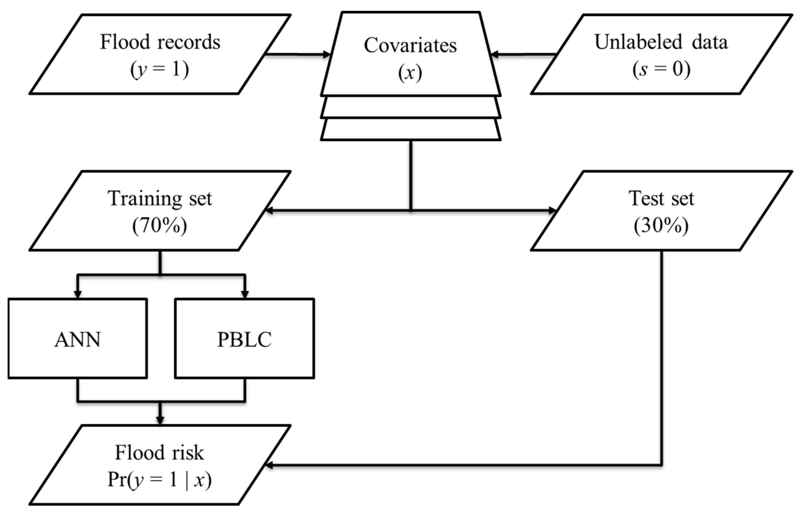
The flood susceptibility or risk magnitude can be defined as a posterior probability conditional on environmental covariates, i.e., Pr(y = 1 | x) where y is a binary response variable and x denotes the environmental covariates. The positive class (flood events) is defined as y = 1 and the negative class (non-flood events) is defined as y = 0. Let s = 1 denote labeled data and s = 0 denote unlabeled data. Unlabeled data are a mixture of positive and negative data, but their true class labels are not known. In the setting of PU learning, only positive data are labeled, but none of the negative data are labeled. Historical records of flood events are positive data (y = 1) and, hence, labeled data (s = 1). The pseudo-negative data collected from the study area are called background samples, treated as unlabeled data (s = 0). Thus, a model trained from labeled positive (s = 1, x) and unlabeled background (s = 0, x) samples can be denoted as Pr(s = 1 | x). In the case-control sampling scenario, the desired model Pr(y = 1 | x) and trained model Pr(s = 1 | x) have the following relationship:
where c is a constant factor indicating the probability of a positive sample being labeled, i.e., Pr(s = 1 | y = 1). Let Pr(s = 1 | x) be a function g of environmental covariates x with parameter of β, i.e., Pr(s = 1 | x) = g(β, x). By minimizing the following loss function, we can infer the parameter β:
where k is the total number of training samples. Let Pr(y = 1 | x) be a function f of x with parameter of ω, i.e., Pr(y = 1 | x) = f(ω, x). According to Equation (1), the loss function in Equation (2) can be rewritten as:
In order to make the parameters ω and c identifiable, a regularization term is added to Equation (3), leading to:
where Pmax is the maximum value of posterior probability and λ is the regularization coefficient. Therefore, we can infer the parameter ω and, hence, the desired model Pr(y = 1 | x) by minimizing the loss function in Equation (4) using positive and unlabeled background data. In practice, we can set the highest flood risk Pmax as one and tune the regularization coefficient λ to make the maximum value of estimated probabilities close to the user-defined value of Pmax. This PU learning algorithm is named positive and background learning with constraints (PBLC) and more details can be found in Li et al. [26].
2.2. Study Area and Dataset
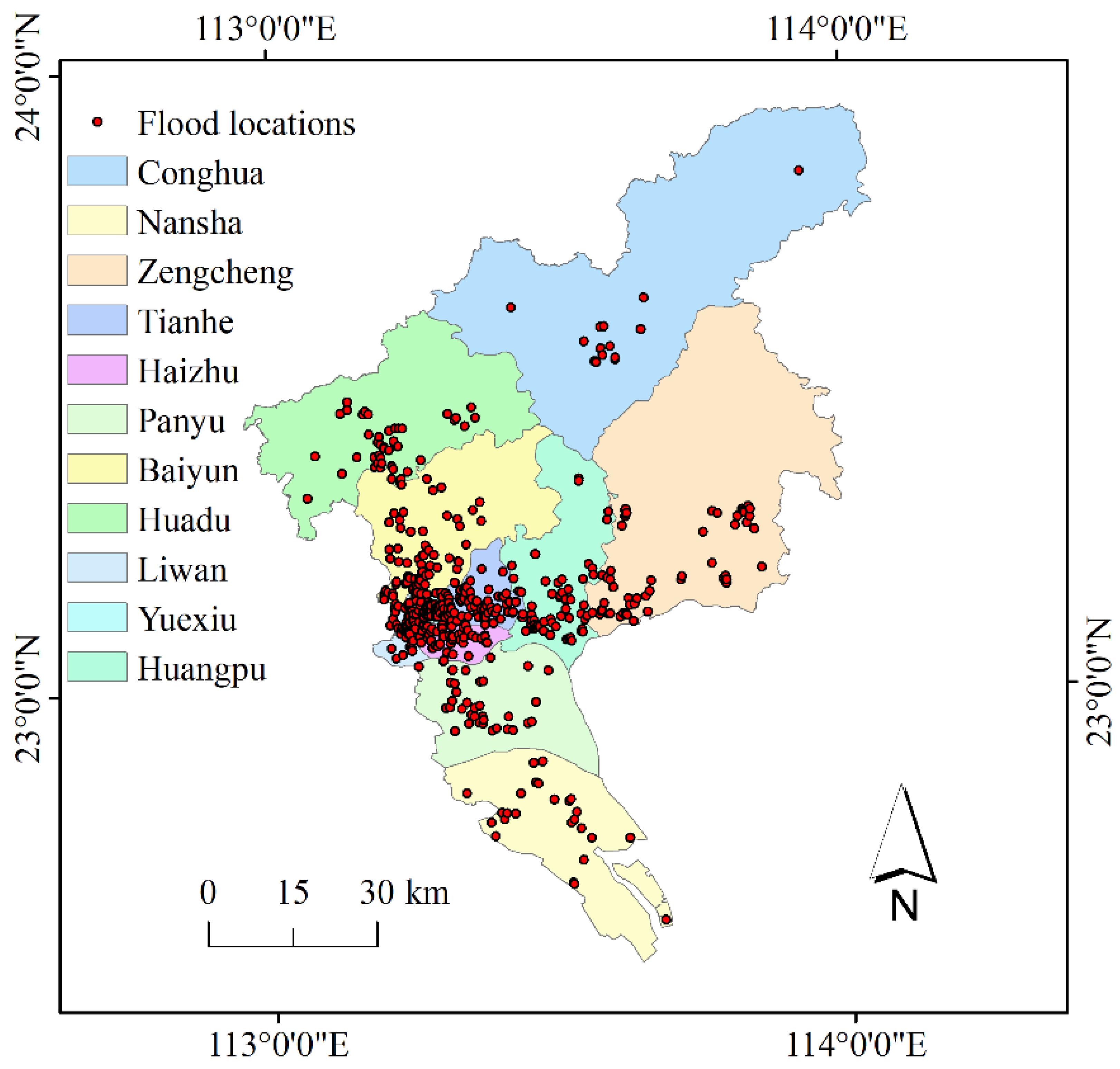
Guangzhou is the capital city of Guangdong Province in Southern China (23°06′32″ N, 113°15′53″ E), with an area of 7434.4 km2. It has a subtropical monsoon climate, with long-term annual mean precipitation of about 1800 mm [27]. Urban flooding events have occurred frequently in recent years [2]. Historical records of flood locations between 2020 and 2022 were collected from the news released by Guangzhou Water Authority. After geocoding and removing outliers, we obtained 532 positive samples shown in Figure 1.
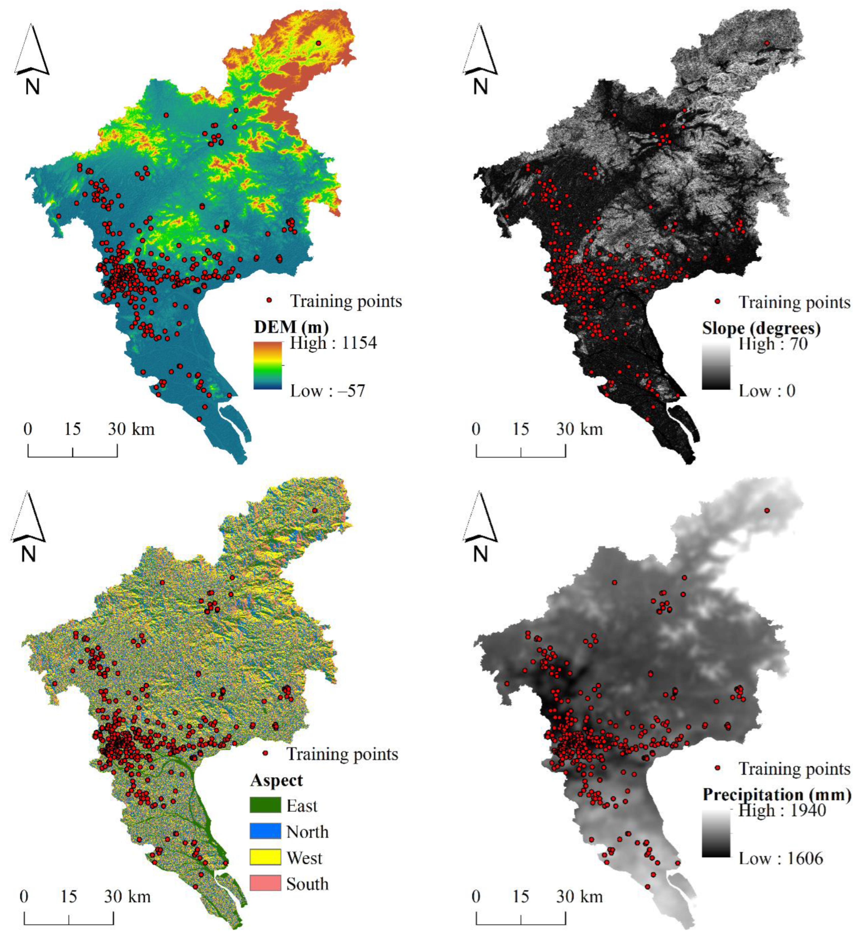
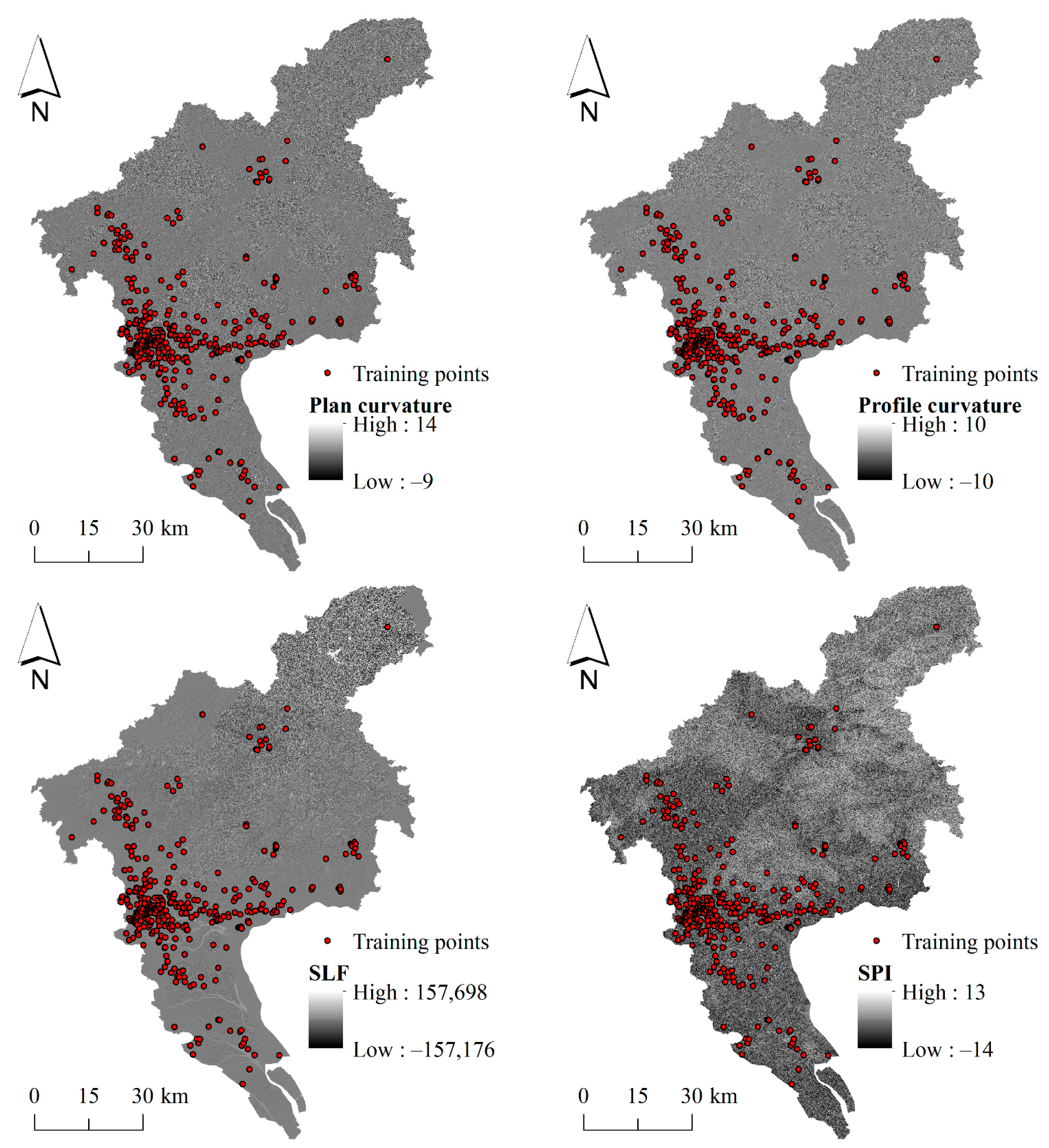
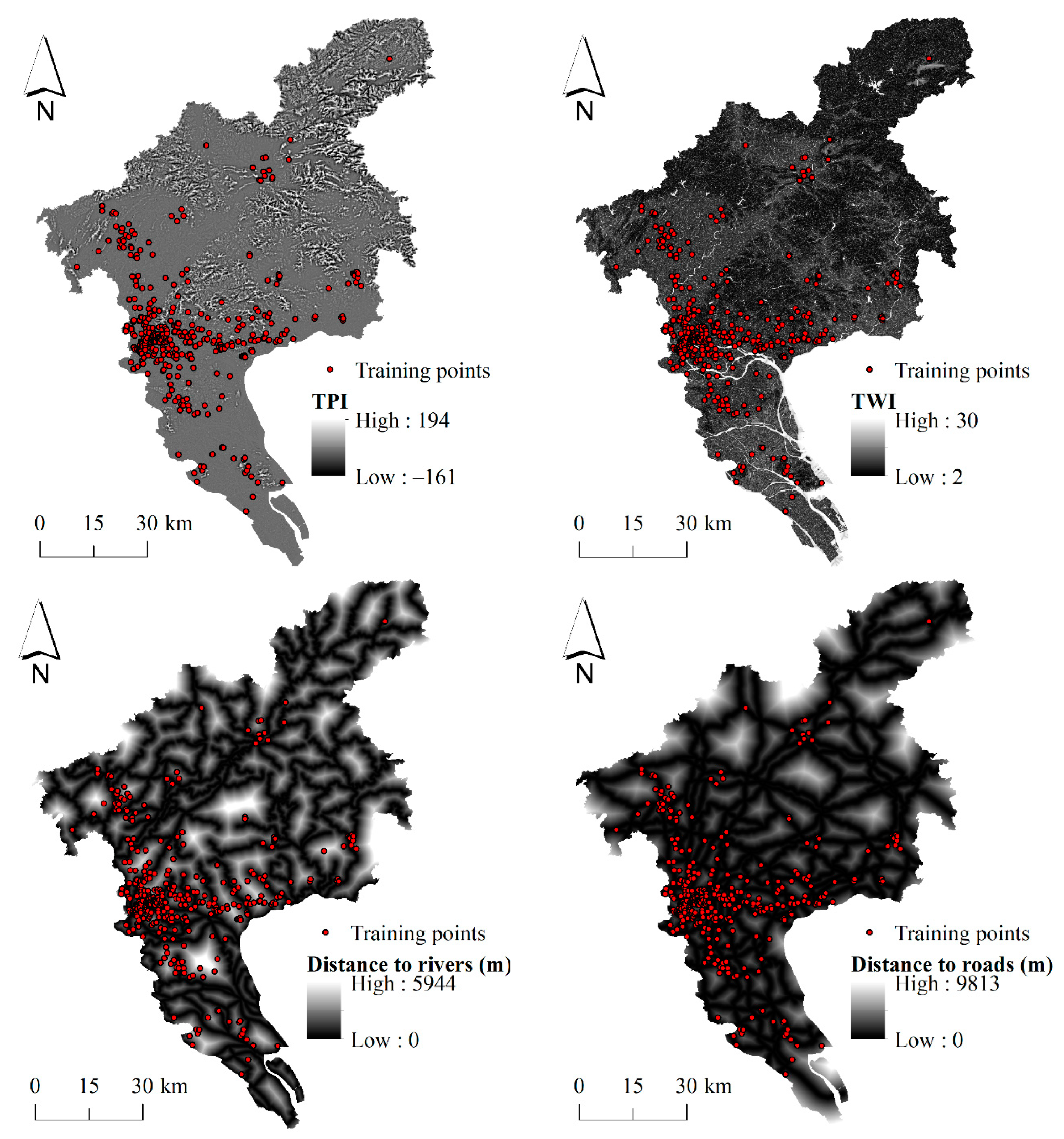
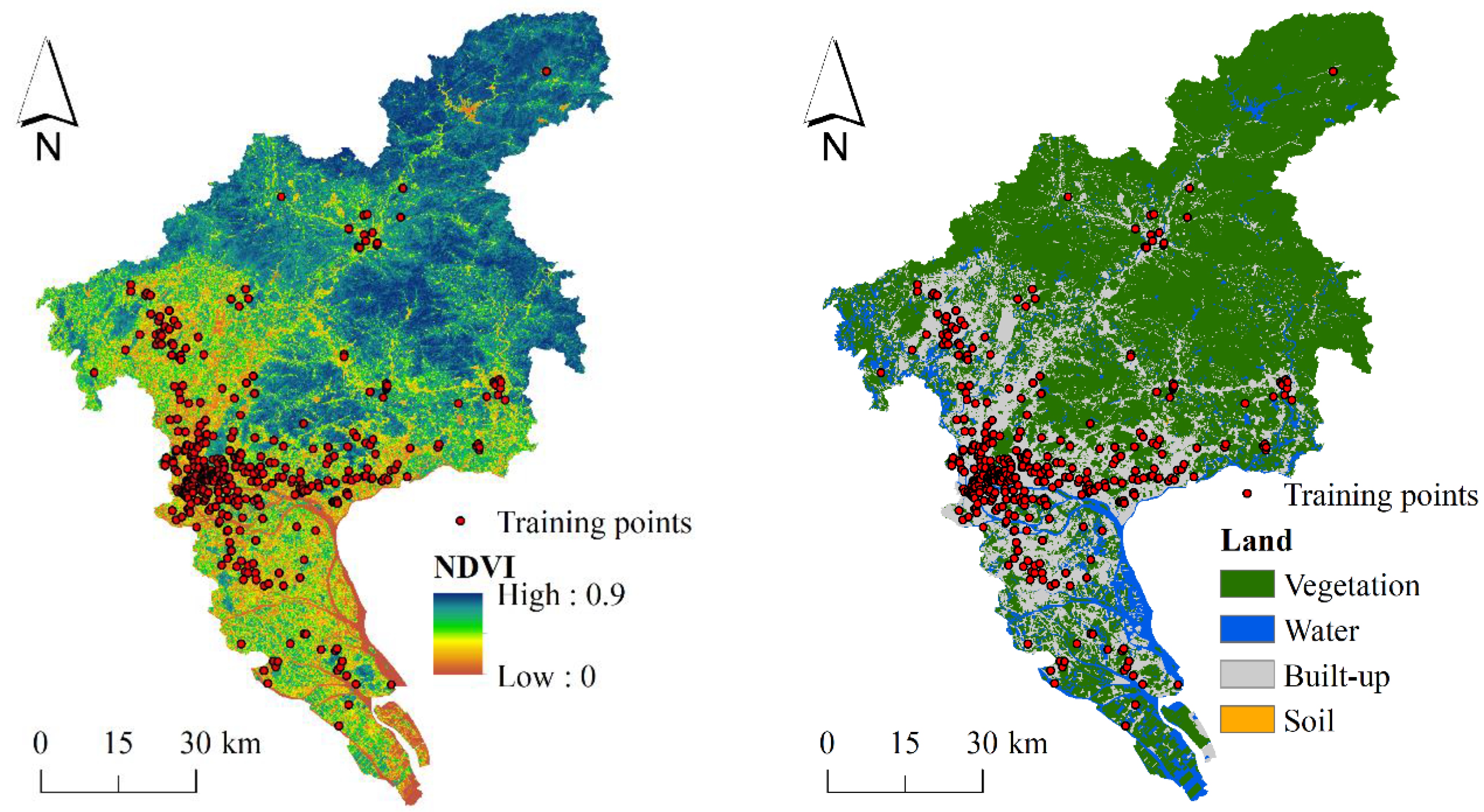
According to the literature and data availability, we selected 14 environmental covariates in this study, including elevation, slope, aspect, plan curvature, profile curvature, slope length factor (SLF), stream power index (SPI), topographic position index (TPI), TWI, distance to rivers, distance to roads, land use, normalized difference vegetation index (NDVI), and precipitation, all of which were preprocessed at a spatial resolution of 30 m. DEM was obtained from U.S. Geological Survey and slope, aspect, plan curvature, profile curvature, SLF, SPI, TPI, and TWI were derived from DEM. The value of aspect ranges from 0 to 360 degrees and we reclassified it into four categories: east, north, west, and south. The vector layers of rivers and roads were obtained from National Geomatics Center of China (http://www.ngcc.cn/ngcc/, accessed on 21 January 2022) and we calculated Euclidean distances to rivers and roads, respectively. Land use map in 2020 was obtained from the GLOBELAND30 (http://www.globeland30.org, accessed on 1 July 2022) and we reclassified the land types into four categories, including water, vegetation, soil, and built up (impervious surface). The mean NDVI (2020–2021) was derived from Landsat8 imagery in Google Earth Engine (GEE) and the mean precipitation (1991–2020) was obtained from Institute of Mountain Hazards and Environment, Chinese Academy of Sciences. Since aspect and land use were categorical features, we converted them into continuous features using the following approach:
where xi refers to the ith category of feature x (i = 1, 2, 3, 4), Pr(xi) refers to the frequency of xi within the whole study area, and Pr(xi | y = 1) refers to the frequency of xi among the positive locations. The maximum value of Spearman’s correlation coefficients between covariates is 0.7939 and the maximum value of variance inflation factor is 5.2747, which indicate that the multicollinearity is low [28]. Therefore, all of the environmental covariates were used for flood susceptibility modeling in this study (Figure 2).
2.3. Model Development
PBLC can be used to train a binary classifier that has the capability to estimate posterior probability, such as logistic regression, ANN, and CNN [26]. Since we only have 532 positive samples in total, the number of samples might not be sufficient to train a complex model, such as CNN. Therefore, we used ANN, which has been widely applied in flood susceptibility modeling, as the classifier in this study.
The recorded flood locations are labeled positive data and unlabeled background data were randomly sampled from the study area. Since non-flood is the majority class in this study area, the number of unlabeled data should be relatively larger to better represent the non-flood class. According to Li et al. (2021), we empirically set the number of unlabeled data as five-times the positive data [26]. The positive and unlabeled data were combined together and we randomly split them into two subsets: 70% for training and 30% for testing. Realizations of training and test sets were randomly repeated 10 times. As a comparison, the ANN model was trained using two different approaches, i.e., traditional supervised learning approach and PBLC, which were named ANN and PBLC, respectively. TensorFlow [29] was used to implement the ANN and PBLC models, with the Adam optimizer [30]. The number of hidden layers was set as two and the number of neurons was 10 for the first hidden layer and 5 for the second hidden layer. The activation function logistic sigmoid was used for the output layer and rectified linear unit was used for other layers. The learning rate was set as 0.005 and the iteration was stopped when training error became stable but validation error started to increase. The validation set was randomly held out from the initial training set (i.e., 25%).
The model performances were evaluated from different perspectives. The area under the receiver operating characteristic curve (AUC) is a threshold-independent measure to evaluate the continuous output [31], whereas F1-score is a threshold-dependent measure to evaluate the binary output [32]. Both AUC and F1-score are traditional measures derived from the confusion matrix requiring an independent test set including both positive and negative data. However, the test set here only consisted of positive and unlabeled data, which also suffered from the problem of contaminated controls. With positive and unlabeled data, the relative value of AUC is still able to rank models, but the absolute value of AUC should be interpreted with caution [33,34]. F1-score does not work with positive and unlabeled data, so we used Fpb instead, which is a proxy of F1-score developed for the case-control positive and unlabeled background data [35]. If a binary model can predict calibrated probabilities, a threshold of 0.5 can generate reasonable binary predictions. Therefore, we applied a threshold of 0.5 to both ANN and PBLC and calculated Fpb to evaluate the predicted accuracies of flood probabilities indirectly. The definition of Fpb is shown in Equation (6):
where TP refers to the number of correctly predicted positive samples, FN refers to the number of positive samples that are falsely predicted as negative, and FP refers to the number of unlabeled samples that are predicted as positive, respectively [35].
In addition, we used the frequency ratio analysis to evaluate the reliability of predicted flood susceptibility levels. The posterior probability of flooding was reclassified to five susceptibility levels with equal intervals: very low (0~0.2), low (0.2~0.4), moderate (0.4~0.6), high (0.6~0.8), and very high (0.8~1). The recorded flood locations in the test set were imposed on the predicted susceptibility map and the relative frequency ratio for susceptibility level i (Ri) is calculated as:
where Fi refers to the percentage of flood points associated with susceptibility level i and Ai refers to the percentage of area with susceptibility level i in the whole study area. The relative frequency ratio should increase from the lowest to the highest level of susceptibility because flooding events are more likely to occur in a higher level of susceptibility zone [36].
Ri = Fi/Ai
The feature importance was also evaluated using the permutation feature importance, which is defined as the decrease in model performance in terms of AUC when a specific feature is randomly permuted [37,38]. The percentage of contribution of a feature, namely Ck, was calculated using the following equation:
where Dk refers to the decrease in AUC when feature k was randomly permuted. Figure 3 shows a flowchart of the experiment.
3. Results
A comparison of model performances by ANN and PBLC is shown in Table 1. The AUC values produced by ANN and PBLC are similar, but the Fpb values produced by PBLC are larger than those from ANN. The average values of AUC by ANN and PBLC over ten random realizations of sample sets are 0.8984 and 0.8974, respectively, whereas the average values of Fpb by both models are 0.7245 and 0.8614, respectively. On average, the minimum, average, and maximum values of predicted probabilities by ANN are 0.0009, 0.1721, and 0.7558, respectively, whereas the minimum, average, and maximum values of predicted probabilities by PBLC are 0.0002, 0.2409, and 0.9775, respectively.
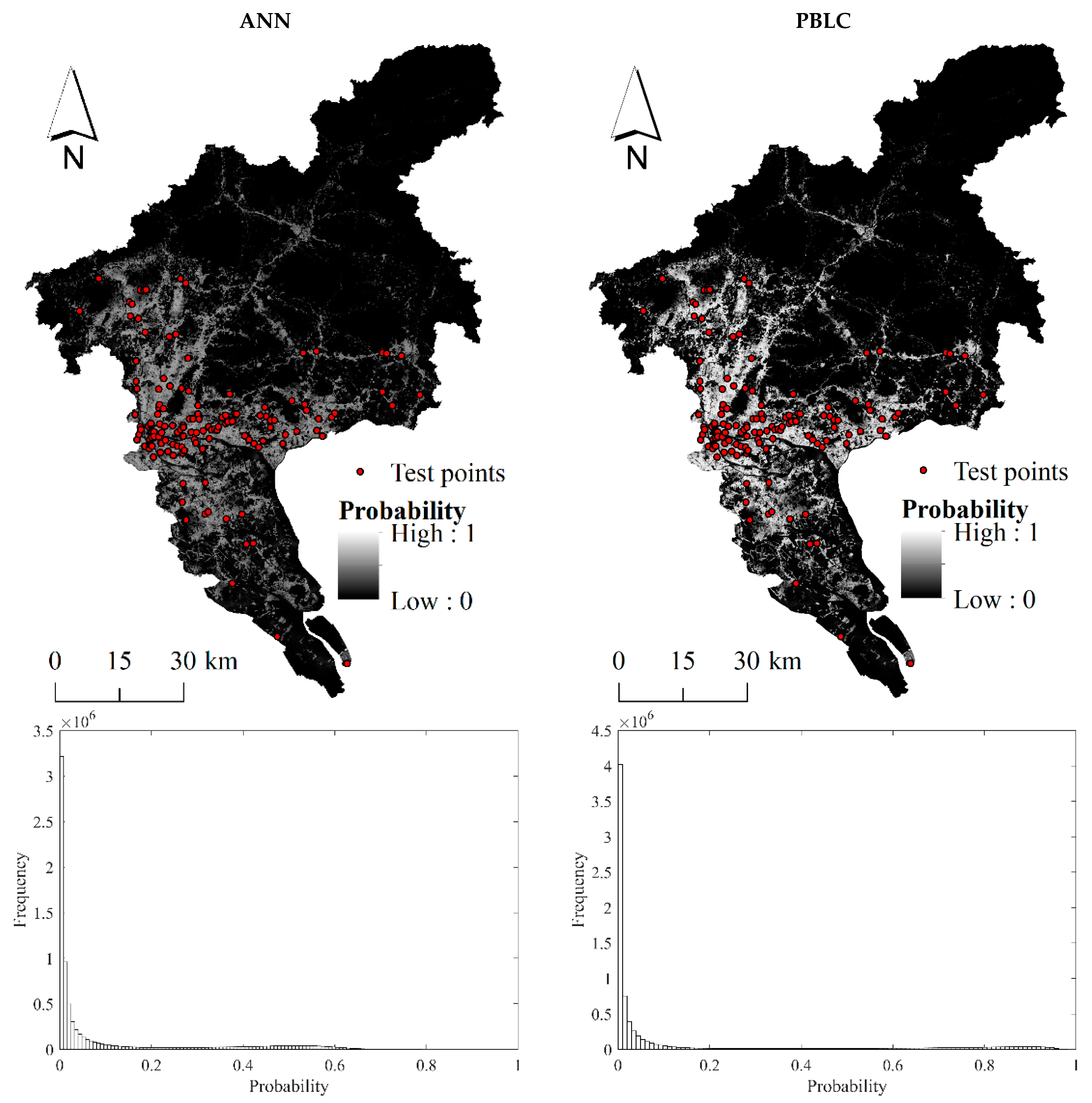
The predicted probabilistic maps of flooding and the corresponding histograms are shown in Figure 4. It is obvious that the predicted probabilities of flooding by ANN are smaller than that by PBLC. In the probabilistic map by PBLC, most of the flood locations in the test set are associated with high probabilities close to one. By contrast, the test points are associated with relatively low probabilities in the prediction map by ANN. The histogram by PBLC also indicates that it produces more calibrated probabilistic predictions covering a range of 0~1. However, the histogram of ANN only covers a range of 0~0.7, indicating that the probabilistic predictions are biased towards zero.
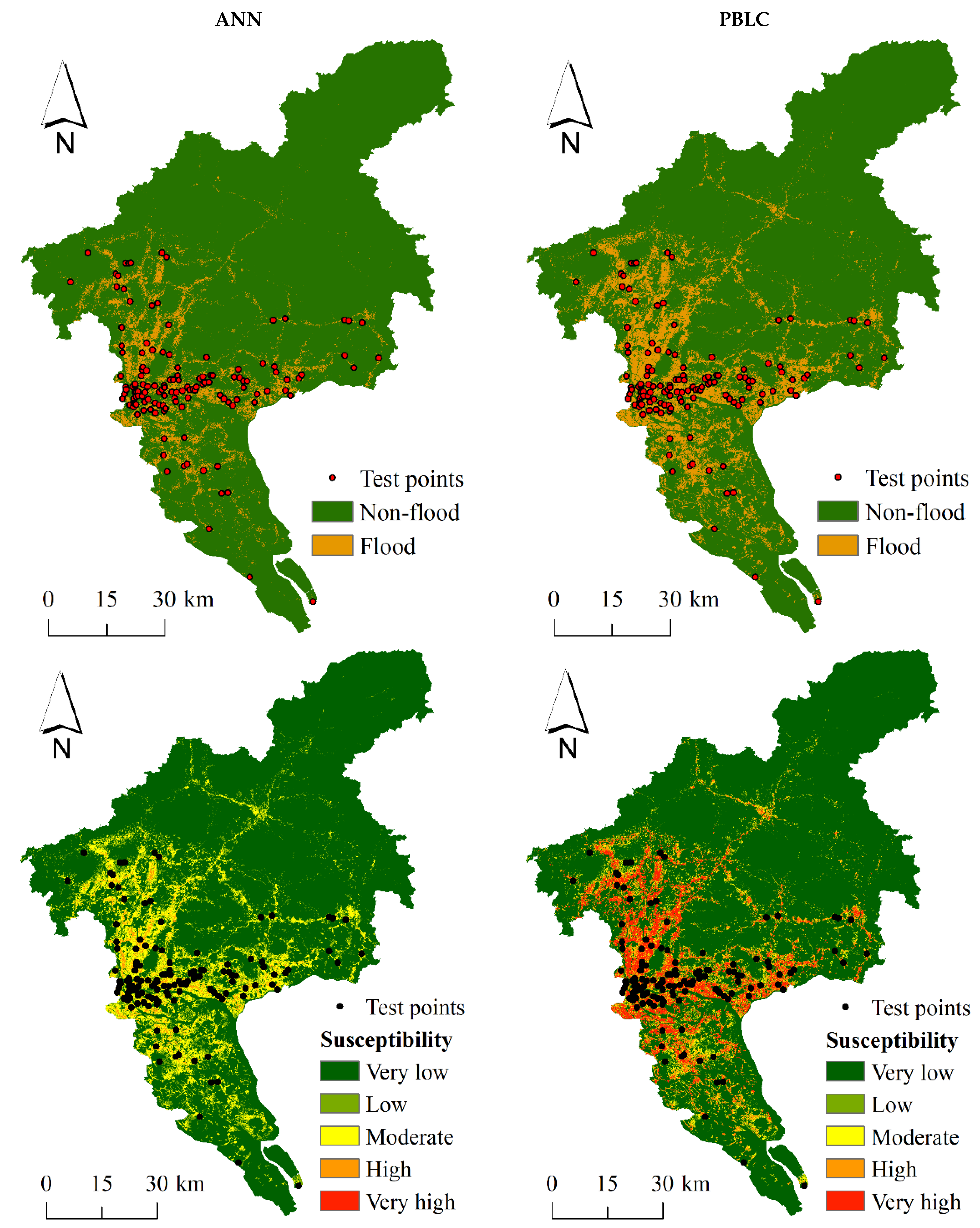
The binary predictions and susceptibility maps of flooding by both models are shown in Figure 5. The predicted flooding area by ANN is much smaller than PBLC, with a large proportion of test points not correctly predicted by the model. In contrast, the predicted flooding area by PBLC is much larger and most of the test points align with the predicted flooding area. Meanwhile, most of the test points fall in the high or very high susceptibility zones in the map predicted by PBLC, whereas most of the test points fall in the moderate susceptibility zone in the map predicted by ANN. According to Table 2, the frequency ratio values by both models increase as the level of susceptibility increases, but the ratio value in the highest susceptibility level predicted by the ANN model is not available because the very high susceptibility zone is not predicted by the model.
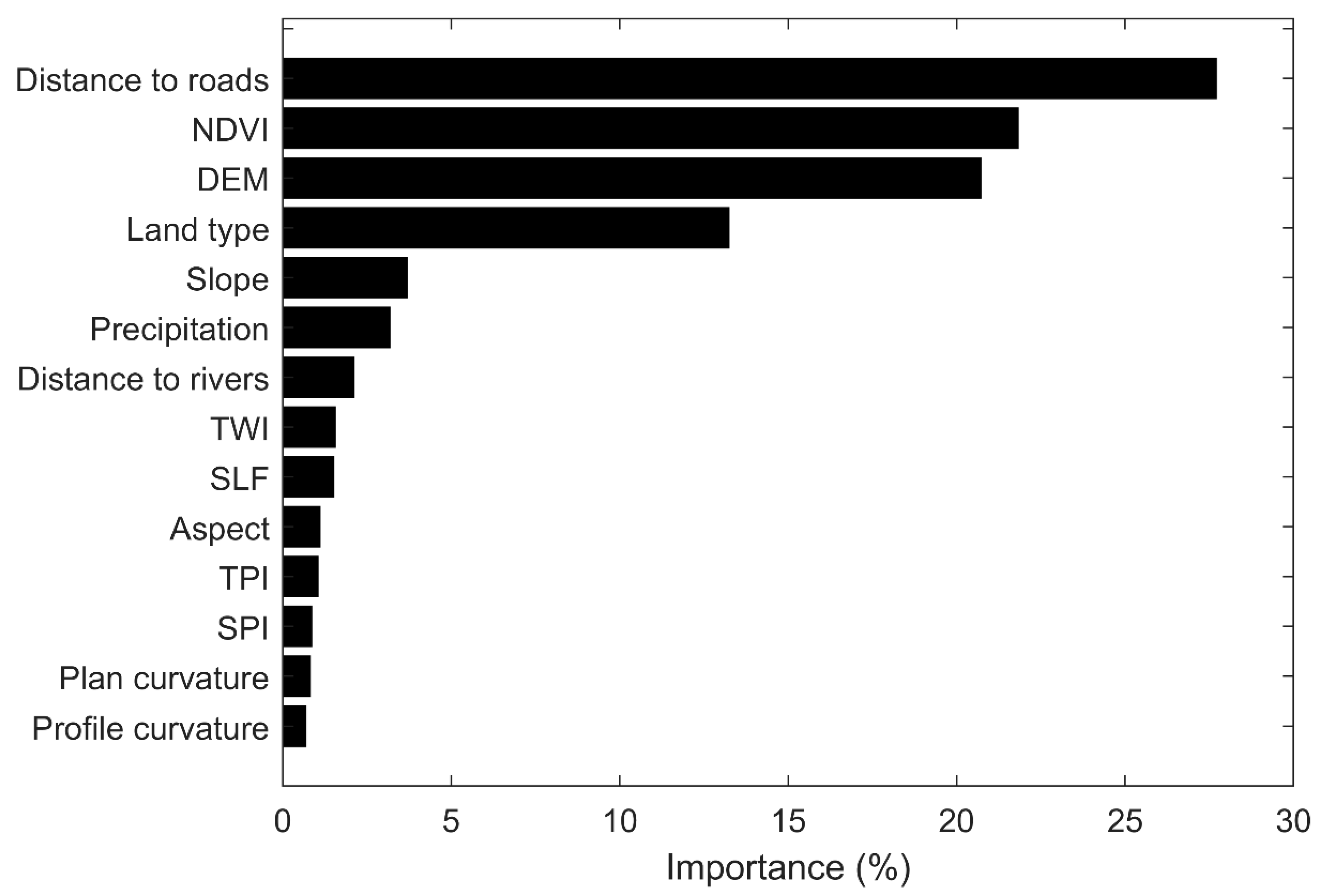
The percentages of flood susceptibility zones in different districts produced by PBLC are summarized in Table 3. The high and very high flood susceptibility zones are mainly located in the central urban districts. For example, the areas of high and very high flood susceptibility zones in the central districts of Yuexiu, Haizhu, Liwan, and Tianhe are all over 47%. In the suburban districts, such as Nansha, Conghua, and Zengcheng, the areas of high and very high flood susceptibility zones are all smaller than 10%. According to Figure 6, the most important influencing factors of flooding in this study area include distance to roads, NDVI, DEM, and land type. The effects of slope, precipitation, and distance to rivers are moderate, whereas the effects of TWI, SLF, aspect, TPI, SPI, plan curvature, and profile curvature are the lowest.
4. Discussion
Machine learning methods have been widely applied in flood susceptibility mapping due to their good abilities to model the complex relationship between influencing factors and flood occurrences. However, traditional machine learning algorithms suffer from the problem of case-control sampling with contaminated controls. Negative (non-flood) samples contaminated by positive (flood) samples will lead to the underestimation of posterior probability Pr(y = 1 | x). If the fraction of positive samples in the training set is not equal to the class prior Pr(y = 1), the estimated posterior probability Pr(y = 1 | x) will be biased. Meanwhile, flooding is usually the minority class in many study areas, so it is very common that the training set contains a small number of flood samples and a large number of non-flood samples, leading to the problem of class imbalance [14]. PU learning has the potential to address these issues because it is designed to learn a classifier from a small set of positive data and a large set of unlabeled data [17], but it has not yet been widely applied and investigated in this field. With a case study in Guangzhou, we show that the novel PU learning algorithm PBLC can be successfully applied in flood susceptibility modeling. PBLC is a flexible model learning approach that could be applied to multiple classifiers, but we only investigate ANN in this study due to the limited size of flood samples. Applications of PBLC to other classifiers, such as CNN, could be further examined when more samples are available.
In this study, the AUC values produced by ANN and PBLC are similar, but the Fpb value produced by PBLC is significantly larger than that by ANN. AUC is a measure of ability to distinguish between positive and negative classes but not a measure of predictive accuracy of probabilities, so it is only related to the relative ranking of predicted scores rather than absolute posterior probabilities [35,39]. According to Equation (1), Pr(s = 1 | x) by ANN is a monotonically increasing function of Pr(y = 1 | x) by PBLC. In other words, the predictions by ANN and PBLC are consistent in ranking, leading to their similar AUC values. By contrast, Fpb is a measure of accuracy of binary predictions, dependent on the selected probability threshold [35]. We can see that the histogram of predicted probabilities by PBLC is more reasonable, whereas the histogram of predicted probabilities by ANN is biased towards zero due to underestimation of probabilities caused by contaminated control samples. As a result, the binary prediction by PBLC with a threshold of 0.5 is more accurate than that by ANN, which explains why PBLC produces a higher value of Fpb than ANN. Meanwhile, the frequency ratio analysis indicates that the predicted susceptibility map by PBLC is more reliable with over 70% of the flood points intersecting high and very high susceptibility zones [1,40], but only 20% of the flood points intersect the high-susceptibility zone with none of the very-high-susceptibility zone being predicted by ANN. Overall, these facts altogether indicate that PBLC provides more calibrated predicted posterior probabilities of flooding than ANN.
Like model training, accuracy assessment also suffers from the problem of case-control sampling with contaminated controls. Please be aware that the relative values of AUC and Fpb can be used to rank model performances, but their absolute values are not truly informative because negative data are replaced by unlabeled data in the test set [33,35]. With positive and unlabeled data, the calculated value of AUC will be smaller than its true value. According to Li and Guo (2021), the constant c can be applied to calibrate the biased AUC value [34]. The estimated value of c provided by PBLC is 0.58 and the AUC value of ANN and PBLC is around 0.90, so the true value of AUC should be around 0.96 after calibration. Similarly, the constant c can also be applied to calibrate Fpb to obtain the unbiased estimate of F1-score [35]. The Fpb values of ANN and PBLC are 0.72 and 0.86, so their true values of F1-score should be 0.65 and 0.73, respectively.
The accuracy assessment shows that the selected environmental covariates are successful in modeling the urban flood susceptibility of Guangzhou. The analysis of feature importance indicates that distance to roads, NDVI, DEM, and land type are the most important conditioning factors of urban flooding in Guangzhou. The recorded flood locations and the high-flood-susceptibility zones predicted by PBLC are mainly located in the central urban districts. Similarly, previous studies also pointed out that most of the flooding events in Guangzhou are concentrated in the central districts, including Yuexiu, Haizhu, Liwan, and Tianhe [2,41]. These areas are characterized by low elevation, high intensity of urbanization, high density of road networks, high imperviousness, and low vegetation cover, all of which could increase the risk of urban flooding [2,42,43]. While previous studies indicate that other factors, such as soil, geology, lithology, and drainage density, can also affect the occurrence of flooding [1,7,23], we do not include these factors in this study because data are not available, which is one of the limitations of our study.
5. Conclusions
In this study, we investigated the effectiveness of a novel PU learning algorithm, namely positive and background learning with constraints (PBLC), in modeling of urban flood susceptibility. Unlike traditional supervised learning that trains a binary classifier from positive (flood) and negative (non-flood) data, the PBLC algorithm trains a binary classifier from positive and unlabeled data. The case study in Guangzhou shows that PBLC can provide more calibrated probabilistic predictions of flooding events than the traditional ANN model and the most important conditioning factors of flooding in Guangzhou include distance to roads, NDVI, DEM, and land type. Our results indicate that PBLC has the potential to address the problem of case-control sampling with contaminated controls that commonly exists in flood susceptibility modeling. We do not investigate the implementation of PBLC with CNN due to the limited sample size and we do not incorporate other factors, such as soil, geology, lithology, and drainage density, which are the limitations of this study. We will investigate these issues when more data are available in the future.
Author Contributions
Conceptualization, W.L., Z.G. and H.H.; methodology, W.L.; data acquisition and analysis, Y.L., Z.L. and W.H.; writing—original draft preparation, W.L.; writing—review and editing, all authors. All authors have read and agreed to the published version of the manuscript.
Funding
This research was funded by the Guangdong Basic and Applied Basic Research Foundation (grant numbers 2020A1515010764 and 2022A1515011494) and the GDAS’ Project of Science and Technology Development (grant number 2022GDASZH-2022010202).
Institutional Review Board Statement
Not applicable.
Informed Consent Statement
Not applicable.
Data Availability Statement
DEM data are available from U.S. Geological Survey (https://www.usgs.gov/, accessed on 7 September 2020). Land use data are available from GLOBELAND30 (http://www.globeland30.org, accessed on 1 July 2022). Most other environmental covariate data are available from National Geomatics Center of China (http://www.ngcc.cn/ngcc/, accessed on 21 January 2022).
Acknowledgments
The authors would like to thank Bintao Liu from the Institute of Mountain Hazards and Environment, Chinese Academy of Sciences for providing the precipitation data. The authors would also like to thank the Editors and anonymous Reviewers for their constructive comments that significantly strengthened this article.
Conflicts of Interest
The authors declare no conflict of interest.
References
- Nkeki, F.N.; Bello, E.I.; Agbaje, I.G. Flood risk mapping and urban infrastructural susceptibility assessment using a GIS and analytic hierarchical raster fusion approach in the Ona River Basin, Nigeria. Int. J. Disaster Risk Reduct. 2022, 77, 103097. [Google Scholar] [CrossRef]
- Huang, H.; Chen, X.; Zhu, Z.; Xie, Y.; Liu, L.; Wang, X.; Wang, X.; Liu, K. The changing pattern of urban flooding in Guangzhou, China. Sci. Total Environ. 2018, 622–623, 394–401. [Google Scholar] [CrossRef]
- Qi, M.; Huang, H.; Liu, L.; Chen, X. Spatial heterogeneity of controlling factors’ impact on urban pluvial flooding in Cincinnati, US. Appl. Geogr. 2020, 125, 102362. [Google Scholar] [CrossRef]
- Rahmati, O.; Pourghasemi, H.R.; Zeinivand, H. Flood susceptibility mapping using frequency ratio and weights-of-evidence models in the Golastan Province, Iran. Geocarto Int. 2016, 31, 42–70. [Google Scholar] [CrossRef]
- Das, S.; Gupta, A. Multi-criteria decision based geospatial mapping of flood susceptibility and temporal hydro-geomorphic changes in the Subarnarekha basin, India. Geosci. Front. 2021, 12, 101206. [Google Scholar] [CrossRef]
- Singha, P.; Das, P.; Talukdar, S.; Pal, S. Modeling livelihood vulnerability in erosion and flooding induced river island in Ganges riparian corridor, India. Ecol. Indic. 2020, 119, 106825. [Google Scholar] [CrossRef]
- Khosravi, K.; Shahabi, H.; Pham, B.T.; Adamowski, J.; Shirzadi, A.; Pradhan, B.; Dou, J.; Ly, H.-B.; Gróf, G.; Ho, H.L.; et al. A comparative assessment of flood susceptibility modeling using Multi-Criteria Decision-Making Analysis and Machine Learning Methods. J. Hydrol. 2019, 573, 311–323. [Google Scholar] [CrossRef]
- Al-Juaidi, A.E.M.; Nassar, A.M.; Al-Juaidi, O.E.M. Evaluation of flood susceptibility mapping using logistic regression and GIS conditioning factors. Arab. J. Geosci. 2018, 11, 765. [Google Scholar] [CrossRef]
- Priscillia, S.; Schillaci, C.; Lipani, A. Flood susceptibility assessment using artificial neural networks in Indonesia. Artif. Intell. Geosci. 2021, 2, 215–222. [Google Scholar] [CrossRef]
- Woznicki, S.A.; Baynes, J.; Panlasigui, S.; Mehaffey, M.; Neale, A. Development of a spatially complete floodplain map of the conterminous United States using random forest. Sci. Total Environ. 2019, 647, 942–953. [Google Scholar] [CrossRef] [PubMed]
- Wang, Y.; Fang, Z.; Hong, H.; Peng, L. Flood susceptibility mapping using convolutional neural network frameworks. J. Hydrol. 2020, 582, 124482. [Google Scholar] [CrossRef]
- Nguyen, H.D. Flood susceptibility assessment using hybrid machine learning and remote sensing in Quang Tri province, Vietnam. Trans. GIS 2022, 1–26. [Google Scholar] [CrossRef]
- Liu, J.; Wang, J.; Xiong, J.; Cheng, W.; Li, Y.; Cao, Y.; He, Y.; Duan, Y.; He, W.; Yang, G. Assessment of flood susceptibility mapping using support vector machine, logistic regression and their ensemble techniques in the Belt and Road region. Geocarto Int. 2022, 1–30. [Google Scholar] [CrossRef]
- Ekmekcioğlu, Ö.; Koc, K.; Özger, M.; Işık, Z. Exploring the additional value of class imbalance distributions on interpretable flash flood susceptibility prediction in the Black Warrior River basin, Alabama, United States. J. Hydrol. 2022, 610, 127877. [Google Scholar] [CrossRef]
- Avand, M.; Moradi, H.; Lasboyee, M.R. Spatial modeling of flood probability using geo-environmental variables and machine learning models, case study: Tajan watershed, Iran. Adv. Space Res. 2021, 67, 3169–3186. [Google Scholar] [CrossRef]
- Li, X.; Yan, D.; Wang, K.; Weng, B.; Qin, T.; Liu, S. Flood Risk Assessment of Global Watersheds Based on Multiple Machine Learning Models. Water 2019, 11, 1654. [Google Scholar] [CrossRef] [Green Version]
- Elkan, C.; Noto, K. Learning classifiers from only positive and unlabeled data. In Proceedings of the 14th ACM SIGKDD International Conference on Knowledge Discovery and Data Mining, Las Vegas, NV, USA, 24–27 August 2008; pp. 213–220. [Google Scholar]
- Hastie, T.; Fithian, W. Inference from presence-only data; the ongoing controversy. Ecography 2013, 36, 864–867. [Google Scholar] [CrossRef] [PubMed]
- Ward, G.; Hastie, T.; Barry, S.; Elith, J.; Leathwick, J.R. Presence-only data and the EM algorithm. Biometrics 2009, 65, 554–563. [Google Scholar] [CrossRef] [Green Version]
- Chapi, K.; Singh, V.P.; Shirzadi, A.; Shahabi, H.; Bui, D.T.; Pham, B.T.; Khosravi, K. A novel hybrid artificial intelligence approach for flood susceptibility assessment. Environ. Model. Softw. 2017, 95, 229–245. [Google Scholar] [CrossRef]
- Lancaster, T.; Imbens, G. Case-control studies with contaminated controls. J. Econ. 1996, 71, 145–160. [Google Scholar] [CrossRef]
- van Engelen, J.E.; Hoos, H.H. A survey on semi-supervised learning. Mach. Learn. 2020, 109, 373–440. [Google Scholar] [CrossRef] [Green Version]
- Zhao, G.; Pang, B.; Xu, Z.; Peng, D.; Xu, L. Assessment of urban flood susceptibility using semi-supervised machine learning model. Sci. Total Environ. 2019, 659, 940–949. [Google Scholar] [CrossRef] [PubMed]
- Bekker, J.; Davis, J. Learning from positive and unlabeled data: A survey. Mach. Learn. 2020, 109, 719–760. [Google Scholar] [CrossRef] [Green Version]
- Li, W.; Guo, Q.; Elkan, C. Can we model the probability of presence of species without absence data? Ecography 2011, 34, 1096–1105. [Google Scholar] [CrossRef]
- Li, W.; Guo, Q.; Elkan, C. One-Class Remote Sensing Classification from Positive and Unlabeled Background Data. IEEE J. Sel. Top. Appl. Earth Obs. Remote Sens. 2021, 14, 730–746. [Google Scholar] [CrossRef]
- Yang, L.; Scheffran, J.; Qin, H.; You, Q. Climate-related flood risks and urban responses in the Pearl River Delta, China. Reg. Environ. Change 2015, 15, 379–391. [Google Scholar] [CrossRef]
- Midi, H.; Sarkar, S.K.; Rana, S. Collinearity diagnostics of binary logistic regression model. J. Interdiscip. Math. 2010, 13, 253–267. [Google Scholar] [CrossRef]
- Abadi, M.; Agarwal, A.; Barham, P.; Brevdo, E.; Chen, Z.; Citro, C.; Corrado, G.S.; Davis, A.; Dean, J.; Devin, M.; et al. TensorFlow: Large-Scale Machine Learning on Heterogeneous Systems. arXiv 2016, arXiv:1603.04467. [Google Scholar]
- Kingma, D.P.; Ba, J. Adam: A Method for Stochastic Optimization. In Proceedings of the 3rd International Conference for Learning Representations, San Diego, CA, USA, 7–9 May 2015; pp. 1–15. [Google Scholar]
- Davis, J.; Goadrich, M. The relationship between Precision-Recall and ROC curves. In Proceedings of the 23rd International Conference on Machine Learning, Pittsburgh, PA, USA, 25–29 June 2006; pp. 233–240. [Google Scholar]
- Goutte, C.; Gaussier, E. A Probabilistic Interpretation of Precision, Recall and F-Score, with Implication for Evaluation. In Proceedings of the Advances in Information Retrieval, Berlin/Heidelberg, Germany, 14–18 April 2005; pp. 345–359. [Google Scholar]
- Jiménez-Valverde, A. Insights into the area under the receiver operating characteristic curve (AUC) as a discrimination measure in species distribution modelling. Glob. Ecol. Biogeogr. 2012, 21, 498–507. [Google Scholar] [CrossRef]
- Li, W.; Guo, Q. Plotting receiver operating characteristic and precision–recall curves from presence and background data. Ecol. Evol. 2021, 11, 10192–10206. [Google Scholar] [CrossRef]
- Li, W.; Guo, Q. How to assess the prediction accuracy of species presence–absence models without absence data? Ecography 2013, 36, 788–799. [Google Scholar] [CrossRef]
- Pradhan, B.; Lee, S. Landslide susceptibility assessment and factor effect analysis: Backpropagation artificial neural networks and their comparison with frequency ratio and bivariate logistic regression modelling. Environ. Model. Softw. 2010, 25, 747–759. [Google Scholar] [CrossRef]
- Altmann, A.; Toloşi, L.; Sander, O.; Lengauer, T. Permutation importance: A corrected feature importance measure. Bioinformatics 2010, 26, 1340–1347. [Google Scholar] [CrossRef] [PubMed] [Green Version]
- Breiman, L. Random Forests. Mach. Learn. 2001, 45, 5–32. [Google Scholar] [CrossRef] [Green Version]
- Lobo, J.M.; Jiménez-Valverde, A.; Real, R. AUC: A misleading measure of the performance of predictive distribution models. Glob. Ecol. Biogeogr. 2008, 17, 145–151. [Google Scholar] [CrossRef]
- Hossain, M.K.; Meng, Q. A fine-scale spatial analytics of the assessment and mapping of buildings and population at different risk levels of urban flood. Land Use Policy 2020, 99, 104829. [Google Scholar] [CrossRef]
- Wang, G.; Liu, L.; Shi, P.; Zhang, G.; Liu, J. Flood Risk Assessment of Metro System Using Improved Trapezoidal Fuzzy AHP: A Case Study of Guangzhou. Remote Sens. 2021, 13, 5154. [Google Scholar] [CrossRef]
- Barbosa, A.E.; Fernandes, J.N.; David, L.M. Key issues for sustainable urban stormwater management. Water Res. 2012, 46, 6787–6798. [Google Scholar] [CrossRef]
- Goonetilleke, A.; Thomas, E.; Ginn, S.; Gilbert, D. Understanding the role of land use in urban stormwater quality management. J. Environ. Manag. 2005, 74, 31–42. [Google Scholar] [CrossRef]
Figure 1.
The distribution of flood locations in each district of Guangzhou.

Figure 2.
The environmental covariates in the study area. Training points refer to the recorded flood locations in the training set.
Figure 2.
The environmental covariates in the study area. Training points refer to the recorded flood locations in the training set.


Figure 3.
The flowchart of the experiment.

Figure 4.
The predicted probabilistic maps of flooding (top row) and histograms of predicted probabilities (bottom row) produced by ANN and PBLC. Test points refer to the recorded flood locations in the test set.
Figure 4.
The predicted probabilistic maps of flooding (top row) and histograms of predicted probabilities (bottom row) produced by ANN and PBLC. Test points refer to the recorded flood locations in the test set.

Figure 5.
The binary predictions (top row) and flood susceptibility maps (bottom row) produced by ANN and PBLC. Test points refer to the recorded flood locations in the test set.
Figure 5.
The binary predictions (top row) and flood susceptibility maps (bottom row) produced by ANN and PBLC. Test points refer to the recorded flood locations in the test set.

Figure 6.
The ranking of permutation feature importance based on PBLC.


Table 1.
Performances of ANN and PBLC over ten realizations of sample sets.
| ANN | PBLC | |||||||||
|---|---|---|---|---|---|---|---|---|---|---|
| Repetition | Prmin | Prave | Prmax | AUC | Fpb | Prmin | Prave | Prmax | AUC | Fpb |
| 1 | 0.0000 | 0.1794 | 0.8162 | 0.8893 | 0.6887 | 0.0014 | 0.2691 | 0.9818 | 0.8888 | 0.8127 |
| 2 | 0.0013 | 0.1788 | 0.8112 | 0.8789 | 0.6891 | 0.0000 | 0.2075 | 0.9695 | 0.8777 | 0.7634 |
| 3 | 0.0000 | 0.1742 | 0.6983 | 0.9033 | 0.7313 | 0.0006 | 0.2410 | 0.9723 | 0.9058 | 0.9299 |
| 4 | 0.0000 | 0.1807 | 0.7597 | 0.9021 | 0.8465 | 0.0000 | 0.2463 | 0.9770 | 0.9015 | 0.8905 |
| 5 | 0.0000 | 0.1648 | 0.7855 | 0.8892 | 0.6601 | 0.0000 | 0.2219 | 0.9704 | 0.8842 | 0.7722 |
| 6 | 0.0014 | 0.1701 | 0.7232 | 0.9017 | 0.7130 | 0.0000 | 0.2391 | 0.9817 | 0.9021 | 0.8848 |
| 7 | 0.0000 | 0.1645 | 0.6877 | 0.9093 | 0.8100 | 0.0000 | 0.2200 | 0.9862 | 0.9095 | 0.8968 |
| 8 | 0.0015 | 0.1814 | 0.7775 | 0.9109 | 0.8411 | 0.0000 | 0.2473 | 0.9620 | 0.9063 | 0.8811 |
| 9 | 0.0017 | 0.1657 | 0.7724 | 0.9027 | 0.6635 | 0.0000 | 0.2499 | 0.9843 | 0.9010 | 0.8811 |
| 10 | 0.0027 | 0.1610 | 0.7264 | 0.8967 | 0.6019 | 0.0000 | 0.2665 | 0.9897 | 0.8967 | 0.9010 |
| AVE | 0.0009 | 0.1721 | 0.7558 | 0.8984 | 0.7245 | 0.0002 | 0.2409 | 0.9775 | 0.8974 | 0.8614 |
| STD | 0.0010 | 0.0078 | 0.0450 | 0.0100 | 0.0826 | 0.0005 | 0.0198 | 0.0087 | 0.0105 | 0.0574 |
Prmin: minimum value of predicted probability. Prave: average value of predicted probability. Prmax: maximum value of predicted probability. AVE: average. STD: standard deviation.
Table 2.
The frequency ratio values for susceptibility maps by ANN and PBLC.
| ANN | PBLC | |||||
|---|---|---|---|---|---|---|
| Susceptibility | Percentage of Flood Points (%) | Percentage of Area (%) | Ratio | Percentage of Flood Points (%) | Percentage of Area (%) | Ratio |
| Very low | 7.69 | 79.10 | 0.0972 | 7.69 | 79.49 | 0.0968 |
| Low | 18.88 | 7.54 | 2.503 | 9.09 | 3.63 | 2.5048 |
| Moderate | 53.15 | 11.59 | 4.5873 | 11.19 | 3.96 | 2.8268 |
| High | 20.28 | 1.77 | 11.4786 | 20.98 | 5.94 | 3.5345 |
| Very high | 0 | 0 | NA | 51.05 | 6.99 | 7.3084 |
Table 3.
The percentages (%) of susceptibility zones in each district of Guangzhou.
| Susceptibility | Yuexiu | Haizhu | Liwan | Tianhe | Baiyun | Huangpu | Huadu | Panyu | Nansha | Conghua | Zengcheng |
|---|---|---|---|---|---|---|---|---|---|---|---|
| Very low | 20.57 | 34.13 | 17.03 | 36.20 | 57.83 | 68.47 | 77.96 | 58.08 | 80.84 | 96.42 | 87.53 |
| Low | 7.86 | 7.69 | 7.18 | 7.47 | 4.60 | 5.66 | 4.20 | 7.94 | 5.52 | 1.30 | 2.32 |
| Moderate | 11.78 | 9.59 | 10.90 | 8.96 | 5.20 | 6.36 | 4.37 | 8.90 | 5.87 | 1.06 | 2.63 |
| High | 25.16 | 17.89 | 22.41 | 16.13 | 10.51 | 9.63 | 6.60 | 12.56 | 6.07 | 0.93 | 4.10 |
| Very high | 34.64 | 30.69 | 42.47 | 31.25 | 21.87 | 9.87 | 6.87 | 12.54 | 1.71 | 0.29 | 3.43 |
| Total | 100 | 100 | 100 | 100 | 100 | 100 | 100 | 100 | 100 | 100 | 100 |
Publisher’s Note: MDPI stays neutral with regard to jurisdictional claims in published maps and institutional affiliations. |
© 2022 by the authors. Licensee MDPI, Basel, Switzerland. This article is an open access article distributed under the terms and conditions of the Creative Commons Attribution (CC BY) license (https://creativecommons.org/licenses/by/4.0/).
Share and Cite
MDPI and ACS Style
Li, W.; Liu, Y.; Liu, Z.; Gao, Z.; Huang, H.; Huang, W. A Positive-Unlabeled Learning Algorithm for Urban Flood Susceptibility Modeling. Land 2022, 11, 1971. https://0-doi-org.brum.beds.ac.uk/10.3390/land11111971
AMA Style
Li W, Liu Y, Liu Z, Gao Z, Huang H, Huang W. A Positive-Unlabeled Learning Algorithm for Urban Flood Susceptibility Modeling. Land. 2022; 11(11):1971. https://0-doi-org.brum.beds.ac.uk/10.3390/land11111971
Chicago/Turabian StyleLi, Wenkai, Yuanchi Liu, Ziyue Liu, Zhen Gao, Huabing Huang, and Weijun Huang. 2022. "A Positive-Unlabeled Learning Algorithm for Urban Flood Susceptibility Modeling" Land 11, no. 11: 1971. https://0-doi-org.brum.beds.ac.uk/10.3390/land11111971
Note that from the first issue of 2016, this journal uses article numbers instead of page numbers. See further details here.