Nonlinear Cooling Effect of Street Green Space Morphology: Evidence from a Gradient Boosting Decision Tree and Explainable Machine Learning Approach

Abstract

Mitigation of the heat island effect is critical due to the frequency of extremely hot weather. Urban street greening can achieve this mitigation and improve the quality of urban spaces and people’s welfare. However, a clear definition of street green space morphology is lacking, and the nonlinear mechanism of its cooling effect is still unclear; the interaction between street green space morphology and the surrounding built environment has not been investigated. This study used machine learning, deep learning, and computer vision methods to predict land surface temperature based on street green space morphology and the surrounding built environment. The performances of the XGBoost, LightGBM, and CatBoost models were then compared, and the nonlinear cooling effects offered by the street green space morphology were analyzed using the Shapley method. The results show that streets with a high level of green environment exposure (GVI > 0.4, NDVI > 4) can accommodate more types of green space morphology while maintaining the cooling effect. Additionally, the proportion of vegetation with simple geometry (FI < 0.2), large leaves (FD < 0.65), light-colored leaves (CSI > 13), and high leaf density (TDE > 3) should be increased in streets with a low level of green environment exposure (GVI < 0.1, NDVI < 2.5). Meanwhile, streets with highly variable building heights (AFI > 1.5) or large areas covered by buildings (BC > 0.3) should increase large leaf vegetation (FD < 0.65) while decreasing dark leaf vegetation (CSI < 13). The study uses machine learning methods to construct a nonlinear cooling benefit model for street green space morphology, proposes design recommendations for different street green spaces that consider climate adaptation, and provides a reference for urban thermal environment regulation.

1. Introduction

Climate change and the surface urban heat island (SUHI) effect exacerbate extreme heat exposure [1,2] and persistently threaten the sustainability of inhabited places [3,4]. With the increase in global urbanization, the population of major cities has increased nearly sixfold in the last 70 years [5], and Asia, home to 54% of the global urban population, is facing a series of challenges that threaten social well-being and quality of life due to global warming [6]. Scholars have put forward various perspectives on mitigating the urban heat island effect, including policy responses and technical solutions. Many of these studies have been focused on urban development, landscape alteration, and exploring the role of blue-green spaces [7]. Notably, the use of urban greening to mitigate the impact of urban heat islands has received increasing attention over the last few years.

As a nature-based cooling strategy for urban areas, vegetated urban green spaces are important components of urban ecosystems and green infrastructure. These spaces can lower temperatures through transpiration effects [8], cool the ground surface by providing shade [9], or absorb greenhouse gases [10]. Essentially, the more vegetation there is and the larger the scale of the urban green space, then the stronger the ability of those spaces to mitigate the effects of urban heat islands [11,12,13]. Research on the use of vegetation to mitigate the effects of urban heat islands has become quite widespread and multidisciplinary [14]. It has included numerical simulations that use computational fluid dynamics (CFD) or energy balance modeling (EBM) software [15,16,17]; field measurements of meteorological parameters (temperature, wind speed, and relative humidity) and vegetation physiological information (tree height, leaf area index, and canopy width) [18,19]; and remote sensing techniques based on ENVI and other software packages to resolve various types of satellite images [20,21]. Additionally, some studies have used a combination of methods. The above studies have confirmed the contribution of green spaces to mitigating the effects of urban heat islands and improving the urban climate.

Several studies have focused on the association between green space morphology and the urban thermal environment; these studies are typically divided into two categories. One type of these studies is based on a network model of landscape ecology; it investigates the influence of the planar morphology of green space on the cooling effect [22], employs remote sensing images to invert the land surface temperature, thus defining the urban heat island [23], then measures the area, proportion, and distance of green space using spatial measurement tools [13,24]. Another type of research, divided into two branches, focuses on the cooling effect of green space morphology in three dimensions, particularly street greens, using field measurements combined with numerical simulations [14]. One of these branches involves simplifying the vegetation shape into a geometric model within the software, then combining it with a building model arrangement to simulate the effect of green space morphology on urban heat islands in a real-world environment [25,26]. In the other branch, the cooling effect of greening morphology is primarily measured by plant physiological parameters such as vegetation height, branch height, and canopy morphology [14,25,26], as well as differences in shade coverage due to differences in tree species [27,28], volume, or leaf color [29,30]. As noted, the description of 3D greening morphologies is more diverse but lacks input from an urban design perspective. It is difficult to accurately characterize the geometrical morphology of vegetation using only simple geometrical models, and the physiological parameters of plants are not clear enough to guide the urban construction process. Therefore, the definition of existing street greening space morphology still needs to be further integrated with the needs of urban design.

In addition, complex relationships surround the cooling effect of greenery morphology, and the views of established studies are not uniform. For example, regarding the cooling effect of vegetation geometry, there are several different views regarding vegetation with scattered [31], moderate [26], and dense forms [30]. Differing perspectives also exist on the cooling effect of canopy density, with some studies claiming that lower canopy density facilitates ventilation and thus mitigates heat islands [32], while others claim that higher canopy density provides denser shade and thus protection from direct solar radiation [30]. All of the above studies are based on more rigorous scientific experiments with a low probability of miscalculation, thus revealing the possibility that the cooling effect of greenery morphology is a nonlinear mechanism.

The influence of a street’s surrounding built environment on the cooling effect of green space has been confirmed. In a plan view, for example, a street’s surrounding built environment is classified by LCZ (local climate zones) [21,33], while in a three-dimensional view, the influence of building height, building density, street width, and other indicators on the cooling effect of green space are studied [34,35,36,37]. All previous studies have explored the interaction effects of streets’ surrounding built environments on the cooling effect of green spaces, but the description of green spaces is relatively simple and lacks a morphological description. It can be said that the interactive influence relationship between street green space morphology and the surrounding built environment has not been thoroughly investigated.

In summary, this paper proposes three research objectives:

(1)

To introduce a morphological theory to quantify street greening space morphology;

(2)

To explore the nonlinear relationship between street greening space morphology and the cooling effect using a gradient-boosting decision tree;

(3)

To exploit explainable machine learning to explore the interaction mechanism between a street’s surrounding built environment and the cooling effect of street green space morphology.

In this study, we propose a method for quantifying street green space morphology and introduce an ensemble learning algorithm to resolve the nonlinear relationship between street green space morphology and SUHIs and the interactions between all their features. The above results can serve urban planners, landscape architects, and decision-makers as a reference for their work and as an applied method for urban physical assessments that support urban planning and street layout and design.

2. Study Area and Data Preparation

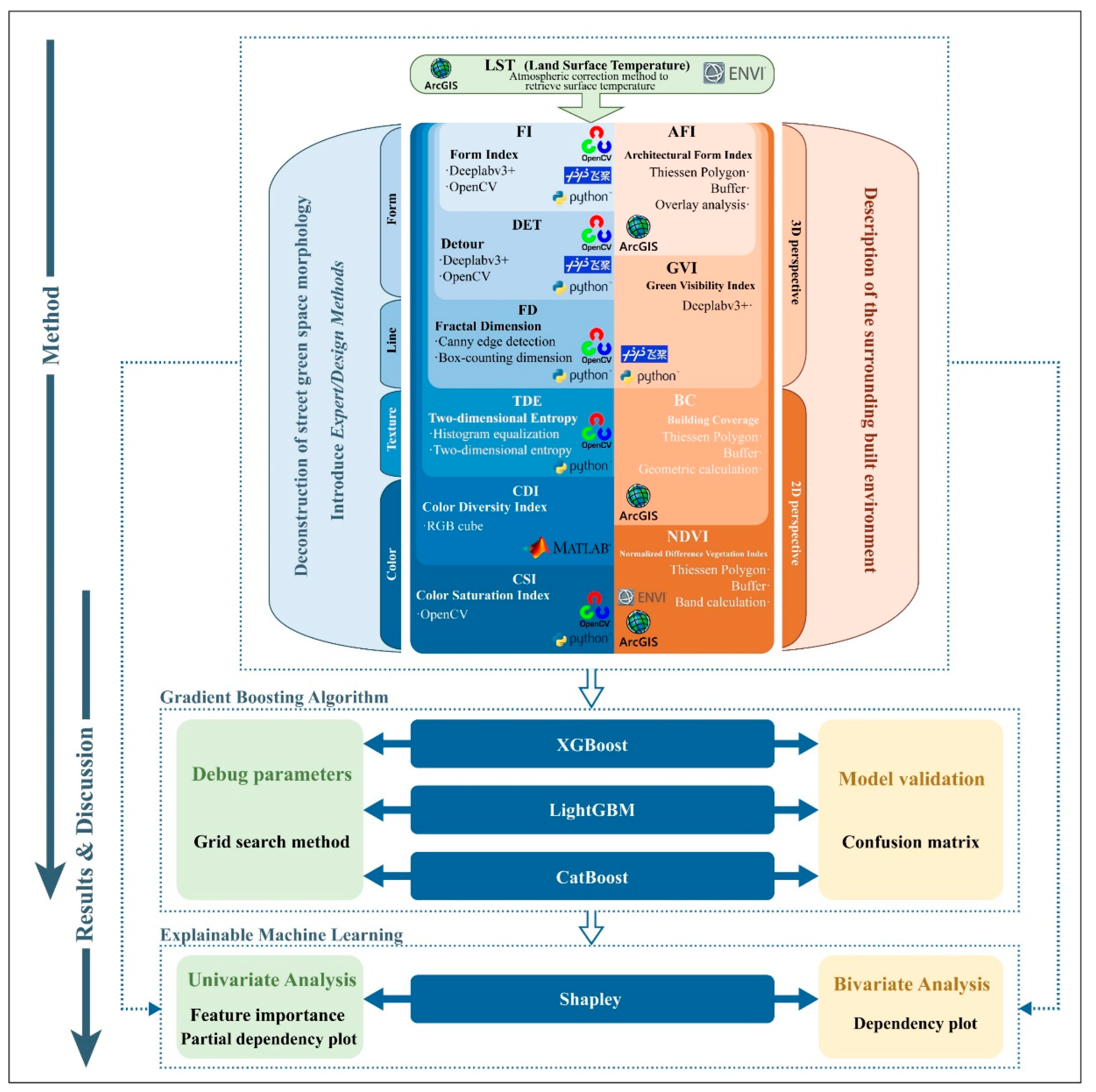
2.1. Overall Research Frame

The specific work presented in this paper is shown in Figure 1 and can be considered in three parts. (1) Expert/design theory, using deep learning and computer vision, is employed to obtain the morphological parameters of street green space. (2) The prediction performances of three models (XGBoost, LightGBM, and CatBoost) that use machine learning methods are compared and the best-performing model is selected to explore the nonlinear relationship between the street green spaces morphology and SUHIs. (3) Feature importance rankings, partial dependency graphs, and dependency graphs are used to resolve the prediction models, interpret the impact of each feature on SUHIs, and propose corresponding urban design countermeasures. The study’s objective is to propose a method for quantifying the space morphology of street green spaces, introduce an integrated learning algorithm to resolve the nonlinear relationship between that space morphology and SUHIs, and examine the feedback, influences, and relationships among all features. The above results can be given to urban planners, landscape architects, and decision-makers as a reference for their work and as an applied method for urban physical assessments to assist urban planning and street layout and design.

2.2. Study Area

The study was conducted within the third ring of Wuhan City, Hubei Province, China, the total length of which is 91 km (Figure 2a). At the end of 2021, the city had a resident population of 10,001,600 and has been commonly known as one of the “Four Furnaces of China” [38]. As a large city located in the middle and lower reaches of the Yangtze River, Wuhan is economically developed, has a rich cultural heritage, has a large and dense population, and has a relatively advanced level of urban construction. Nevertheless, Wuhan is located in a geographical area with frequent high temperatures and poor comfort. In recent years, the heat island effect has intensified with Wuhan’s accelerated urban construction process. The streets within the third ring road of Wuhan are not only diverse in style but also have a rich green configuration. This is the paradigm for many large urban cores. Therefore, it would be beneficial to carry out a study here to draw general conclusions.

2.3. Data Collection

The Open Street Map website (http://www.openstreetmap.org, accessed on 7 June 2022) was used to obtain the geospatial information for 752 main streets in the third ring area of Wuhan, which have a total length of 1981,165 km. The total study area covers 524,813 km², of which the internal neighborhood roads were not included in the analysis. After removing the photos taken in tunnels, in viaducts, or under poor lighting conditions, 15,199 valid street images were obtained.

Remote sensing datasets from the Geospatial Data Cloud (http://www.gscloud.cn, accessed on 11 August 2022) were used to derive the surface temperature. Images of Wuhan city with less than 5% cloud cover taken by Landsat 8, which has a 30 m resolution, on 15 September 2018, were deemed suitable for conducting this study due to the limited cloud coverage in the images.

The dataset used to indicate the building factors is the open-source building outline vector data for major, medium, and large cities in China. The data are stored in the shapefile format.

2.4. Data Preprocessing

As shown in Figure 3, cars were first removed from the streetscape images (which were 4096 × 1536 pixels in size) to eliminate the interference they cause, and the image size was then reduced to 4096 × 1280 after cropping. Then, the deep learning platform was used to build the deeplabV3+ framework, and the semantic segmentation of the streetscape image was performed based on the city spaces dataset developed by urban research. The city spaces dataset supports classifying street scenes into 19 categories, and in this study, only the segmentation results for the label “vegetation” were retained in the segmentation. The corresponding vegetation parts in the street scene images were extracted based on the labeled images using OpenCV, and the other portions of the images were filled with white (RGB = 255, 255, 255).

3. Methods

3.1. Surface Temperature Inversions

Established studies have shown that the apparent temperature, near-surface air temperature, and surface temperature all show a significant correlation [27,28]; therefore, reducing the surface temperature can effectively mitigate the SUHI effect. In this study, land surface temperature (LST) was used to quantify SUHI. The surface temperature inversion was performed in the ENVI software package, and the process was divided into calculating the spectral radiance of the thermal band, calculating the blackbody radiant brightness, and finally calculating the blackbody brightness temperature, i.e., the surface temperature. First, the spectral radiance of the thermal band was obtained by radiometric correction in the thermal infrared band using the following equation:

$$L_{\lambda }=DN\ast Gain+Offset$$

(1)

where L_λ is the spectral radiance of the thermal band, DN is the original pixel value in the thermal infrared image, and Gain and Offset are available in ENVI. Then, water vapor effects are removed by atmospheric correction to obtain the blackbody radiant brightness.

$$B(T_s)=\frac{[L_{\lambda }-L_{up}-\tau \ast (1-\epsilon )\ast L_{down}]}{\tau \ast \epsilon }$$

(2)

where B(T_s) is the blackbody radiance brightness, L_up is the atmospheric outgoing radiation, L_down is the atmospheric incoming radiation, and τ is the atmospheric transmittance, which can be calculated by the NASA atmospheric calculator website (http://atmcorr.gsfc.nasa.gov/, accessed on 11 August 2022), and ε needs to be obtained by the normalized differential vegetation index (NDVI, see Section 3.2.2 for calculation method). Finally, the blackbody radiance is calculated as follows:

$$T_s=\frac{C_2/\lambda }{\ln (\frac{C_1\ast {\lambda }^{-5}}{B(T_s)}+1)}$$

(3)

where T_s is the blackbody radiation brightness, i.e., the surface temperature; C₁ and C₂ are the Plank function parameters, and λ is the effective wavelength.

Then, we constructed grid cells based on the sampled points of the street view images. We used the intersecting area of the Tyson polygon grid at each sampling point and the 80 m buffer as the grid cell and calculated the weighted average ground surface temperature (LST) within each grid cell with the following formula:

$$LS{T}_{\mathrm{i}}=\frac{{\displaystyle \sum _{j=1}^n{A}_{ij}{T}_j}}{A_i}$$

(4)

where LST_i is the weighted average surface temperature within grid cell i, n is the total number of temperature value types within grid cell i, A_i is the area of grid cell i (m2), A_ij is the area occupied by the jth temperature within grid cell i (m²), and T_j is the surface temperature value of the jth temperature (°C). The visualization of the calculation results is shown in Figure 2c.

We combined the histogram of LST (Figure 2b) with the ideas of Suonan [39] and Song [40] to determine the distribution of LST labels shown in Figure 2d, where 0 represents the LST in the normal range (30–38 °C) and 1 represents the LST in the high-temperature region (38–48 °C). The rationale for this classification is to avoid classifying more regions above 38 °C as “0” while ensuring that the difference in the number of the binary labels is as small as possible without affecting model training, thus preventing contradiction with Song’s research. According to Suonan’s research, the monthly relative humidity in Wuhan city has been fairly stable over the past 50 years, while the average relative humidity in September is approximately 78%, and the apparent temperature at this humidity will be much higher than the air temperature. T_ls was calculated to be approximately 34 °C using the linear regression fitting formula for surface temperature (T_ls) and air temperature (T_a) in Song’s study: T_a = T_ls × 0.63 + 4.84 (R² = 0.89) and combined with the optimal outdoor temperature of 26 °C (at 40% humidity) for Chinese residents. The temperature data were provided by China Meteorological News (http://www.zgqxb.com.cn/, accessed on 22 September 2022). However, there is a lag effect of T_a, i.e., when T_ls reaches the maximum value (13:30), Ta will continue to rise over the next 2 h. The remote sensing image used in this study was taken at 14:55, and the calculated T_ls will be lower than the actual maximum T_ls for this time of the day. Finally, we chose the LST value greater than 37 °C as the high-temperature threshold in this study based on the histogram distribution of LST and after considering the viewpoints of various researchers.

3.2. Quantitative Methods for Predicting Indicators

In this section, a total of ten indicators were proposed as independent variables for this study. Of the ten indicators, six variables describe the characteristics of the space morphology of street greenery itself, and the other four indicators describe the surrounding built environment from two-dimensional (2D) and three-dimensional (3D) perspectives to complement it. We deconstructed the morphology of street green spaces from four perspectives: form, line, texture, and color, based on the expert/design theory of extracting the morphological characteristics of the landscape [41,42]. Additionally, considering that the differences in shadow and light intensity generated by buildings impact the line, texture, and color of the morphology of street green spaces [35,43], the building area (2D) and building height (3D) covering the ground surface were included as architectural factors in the quantification process. In addition, previous studies have pointed out the association between green environment exposure and vegetation cooling effects [11,44], and we added normalized difference vegetation index (NDVI) (2D) and green view index (GVI) (3D) to improve the accuracy of describing the street green space morphology.

3.2.1. Methods for Quantifying Street Green Space Morphology

Previous studies have shown that street surface temperature is highly correlated with vegetation morphological characteristics, not only in terms of canopy shape but also in terms of leaf size and leaf color depth [26,29,30,31,45]. However, the measurement of vegetation morphological characteristics often requires fieldwork, which is limited by the high labor cost and the lack of sufficient measurement areas. Similarly, the definitions of morphological characteristics differ from one study to another. Moreover, we aim to assist in the design of street green spaces and will introduce theories and standards in related fields to support the research goals. In this work, “morphological characteristics” refers to the four aspects of form, line, texture, and color, while “geometry” is a collective term for form index (FI) and degree of detour (DET) (

Table 1. Definition and equation of space morphology indicators of street greening.

Variable Name	Description and Implementation Methods	Meaning	Equations	Equation Definition
1.FI	Form index (FI). Semantic segmentation is performed on the street image and the perimeter and the area of each individual color block as well as the Shannon entropy are calculated.	The higher the FI, the more complex the vegetation geometry, or the less coherent the green space.	$FI=-{\displaystyle \sum _{i=1}^n\frac{C_i{P}_i}{S_i}\log P_i}$	where n is the total number of color blocks in the picture, Pi is the proportion of the ith color block in the picture, Ci is the perimeter of the ith color block, and Si is the area of the ith color block.
2.DET	Degree of detour. Semantic segmentation is performed on the street image and the total perimeter to total area ratio of the color blocks is calculated.	The higher the DET, the more complex the vegetation geometry.	$DET=\frac{{\displaystyle \sum _{i=1}^n{C}_i}}{{\displaystyle \sum _{i=1}^n{S}_i}}$	where n is the total number of color blocks in the picture, Ci is the perimeter of the ith color block, and Si is the area of the ith color block.
3.FD	Fractal dimension. The fractal dimension of the street view image is calculated after the edge detection process.	A measure of the size and density of vegetation leaves, the higher the FD the smaller or denser the leaves.	$FD=\underset{\epsilon \to \infty }{\lim }\frac{\log (N({\epsilon }_n))}{\log (1/{\epsilon }_n)}$	Using a grid matrix to cover the image, where the grid edge length is ε and the number of grids N(ε), when the grid is reduced enough to record all εn and N(ε) changes, a scatter coordinate plot is drawn based on log(1/εn) and log(N(εn)), and the slope of the fitted line is recorded as the FD of the graph.
4.TDE	Two-dimensional entropy. The grayscale values of each pixel and its surrounding eight pixels are recorded as a binary group and the Shannon entropy of the binary group is calculated.	A measure of the effect of light and shade produced by vegetation due to the concave and convex variation of its surface density differences. Generally speaking, the denser the surface (canopy) the higher the amount of light received, i.e., the higher the TDE.	$j=\frac{{\displaystyle {\sum }_{k=1}^{8}j(k)}}{8}$ $TDE=-{\displaystyle \sum _{i=0}^{255}{\displaystyle \sum _{j=0}^{255}{p}_{ij}\log p_{ij}}}$	where I denotes the i-th pixel gray value in the picture (i ∈ [0,255]), j is the neighborhood gray value (j ∈ [0,255]), and Pij is the probability that the binary group (i,j) appears in the picture.
5.CDI	Color diversity index. The RGB equation is set, and the eligible pixels are filtered, and the product of the maximum value in the RGB value of the pixel and its grayscale value of Shannon entropy is calculated.	The diversity of pixels with different brightness and saturation at the same hue is recorded, measuring the depth of leaf color. Higher CDI indicates brighter leaf color.	$\begin{array}{l}CDI=-{\displaystyle \sum _{i=1}^n{C}_i{P}_i\log P_i}\\ R^2+(G-255)+B^2<{\left(\frac{255}{2}\right)}^2\end{array}$	where Ci is the color metric of pixel i, Pi is the probability that the grayscale value of pixel i appears in the grayscale image, and Hc is the color information value of this image. R, G, and B correspond to the red, green, and blue color channel values in RGB color mode, respectively, and R ∈ [0,128]; G ∈ [127,255]; and B ∈ [0,128]. When the RGB value of pixel i satisfies the equation below, the maximum value in the RGB value of the pixel is selected as Ci.
6.CSI	Color saturation index. Saturation is calculated from the three RGB channels.	Using saturation to measure the degree of leaf color vividness, the greater the saturation, the more vivid the leaf color or the better the light conditions.	$\begin{array}{l}rg=R-G\\ yb=\frac{1}{2}(R+G)-B\\ {\sigma }_{rgyb}=\sqrt{{\sigma }^2{}_{rg}+{\sigma }^2{}_{yb}}\\ {\mu }_{rgyb}=\sqrt{{\mu }^2{}_{rg}+{\mu }^2{}_{yb}}\\ CSI={\sigma }_{rgyb}+0.3\ast {\mu }_{rgyb}\end{array}$	where R, G, and B correspond to the red, green, and blue color channel values in RGB color mode, respectively, while σrg and σyb are the standard deviations of rg and yb, respectively, and μrg and μyb are the mean values of rg and yb, respectively.

).

Expert/design theory starts from the core of the “human viewer” and proposes that the two most important factors are the “locations” where the observer is located and the “visual sensitivity” of the observed scene. In this study, the streetscape sampling points were arranged at equal distances along the road centerline, which could control the uncertainty of “location” to the maximum extent. The theory deconstructs scenic characteristics in terms of abstract parameters at four levels: form, line, texture, and color, which is a response to the “visual sensitivity” [42]. The measurement can only be carried out manually due to the technological limitations and processing time required and is therefore considered to be too subjective [41]. However, subsequent scholars have argued that the concept of the method is useful for extracting scenic morphological characteristics [46,47]. Currently, with the help of deep learning platforms and computer vision techniques to replace manual labor, the need for objective measurements can be satisfied, and open access to street view images has become the basis for large-scale research. Table 1 and Figure 4 shows the construction and interpretation of the relevant features. In addition, we show the comparison and verification between the calculation results and the actual scene in Appendix A.

From the perspective of information gain, obtaining the main contour features of the image can achieve the purpose of identifying the target object, and the other internal lines added afterward only achieve a detailed description and do not contribute to the recognition of the object itself [36]. This view fits well with the semantic segmentation principle of deep learning [48]. Therefore, for the description of morphological characteristics, we processed the semantic segmentation of the images through the OpenCV framework to obtain the color block perimeter and area values and calculate the FI (form index) and DET (degree of detour) to describe the vegetation geometry. Because all vegetation is largely coherent, there may only be one “vegetation” label color block in the calculation of the FI, resulting in a calculation result of 0. The reason for adding the DET is to supplement the defect of the FI calculation method. The other details of the object are described in the following sections with regard to lines, texture, and color.

Ma et al. used an edge detection algorithm to measure the line features of the scene [49,50], confirming the feasibility of the method. The field of computer vision usually focuses on the main contours of objects in edge detection work. However, we extracted the complete contour of vegetation leaves by adjusting the parameters (such contours are often treated as redundant information in other work). First, the OpenCV interface was invoked in the Python environment to implement Canny edge detection, setting the minimum and maximum thresholds to 100 and 256, while the Sobel operator (convolution kernel) size was set to 3, and the image gradient magnitude was chosen to be of the L1 norm. Finally, the FD (fractal dimension) of the processed image was calculated.

Texture, a more abstract variable, is primarily produced by the variations in light and darkness brought on by the undulations of an object’s surface. Drawing inspiration from the field of computer vision, we traversed the whole image with a 3 × 3 pixel matrix similar to a “convolution kernel” and recorded the value of each matrix so that the spatial attributes could be included in the calculation. However, color images are usually three-channel objects (e.g., RGB, HSV, etc.), and the three-dimensional matrix increases the dimensionality of the operation, thereby reducing the interpretability of the model. Therefore, we introduced the method of quantifying image texture from the field of communication engineering [51,52,53], converted color images into grayscale images of black and white channels (binarization) to reduce their dimensionality, and used each pixel matrix as a unit to calculate its information entropy to obtain the TDE (two-dimensional entropy).

Continuing the concept of TDE, we also adopted a dimensionality reduction operation for the color quantization [54]. First, a three-dimensional coordinate system was established based on the RGB channel, whose x-axis, y-axis, and z-axis are all defined as integers between 0 and 255, and the green color range was defined according to the equations shown in Table 1. When the RGB value of a pixel was included in these ranges, the maximum value in RGB was extracted as the color weight coefficient. At this point, the RGB dimension dropped from three dimensions to one dimension. Next, the image was converted to a grayscale image, and the information entropy of that grayscale pixel was calculated and multiplied with the previously obtained color weight coefficients to obtain the CDI (color diversity index).

Different from CDI, CSI (color saturation index) is derived from a psychophysical experiment by Hasler et al., which used an algorithm to simulate how human eyes perceive color saturation [55]. He used the RGB channel values as the basic parameter to quantify the seven levels of image color evaluation by the subjects, and finally got the “coloriness” of the image, namely CSI.

3.2.2. Methods for Quantifying the Surrounding Built Environment

The surrounding built environment around the street, as the substrate upon which the green spaces are located, also has an important influence on the urban climate and environment. The inclusion of the surrounding environmental variables can complement and modify the analysis results of this study by combining 2D and 3D views, as well as obtaining more comprehensive conclusions.

Table 2. Definitions and equations of peripheral surrounding built environment indicators.

Variable Name	Description and Implementation Methods	Meaning	Equations	Equation Definition
1.GVI	Green view index. Calculates the proportion of pixels in the “vegetation” labeled blocks in the semantic segmentation image.	The higher the GVI, the higher the proportion of vegetation in the field of view.	$GVI=\frac{V_{\mathrm{area}}}{W\ast H}$	Where Varea is the number of image elements of the tag “vegetation” element, W is the image width, and H is the image height.
2.AFI	Architectural form index. Calculates the product of the information entropy of building heights within a grid cell and the total building height.	The building form around the sampled points of the street view image is measured and used as a complementary description of the building shadows in the street canyon -. The higher the AFI, the greater the building interface skyline variation.	$AFI=-{\displaystyle \sum _{i=1}^n{H}_{sum}{P}_i\log }{P}_i$	where Hsum is the sum of building heights in the grid, and Pi is the ratio of the height of the ith building to the total building height.
3.BC	Building coverage area. Calculates the area of the building footprints (i.e., the area covering the ground surface in the grid cell).	The area of impervious paving surface around the street was measured to complement the temperature impact of buildings around the street.	$BC=\frac{A_{\mathrm{buildings}}}{A_{\mathrm{grid}}}$	Where Abudings is the total building area covering the surface in the grid, and Agird is the area of that grid.
4.NDVI	Normalized difference vegetation index. Calculate the weighted average of the vegetation cover degree C within the grid cell.	The degree of vegetation cover around the street was measured, complementing the effect of the street surroundings on temperature.	$\begin{array}{l}C={\displaystyle \sum _{i=1}^n[\frac{(NI{R}_i-RE{D}_i)}{(NI{R}_i+RE{D}_i)}]}\\ NDVI=\frac{{\displaystyle \sum _{j=1}^n{A}_{ij}{C}_j}}{A_i}\end{array}$	Where C is the normalized differential vegetation index, NIRi is the NIR band value of the ith pixel in the grid, and REDi is the red band value of the ith pixel in the grid. Ai is the area of grid cell i (m2), Aij is the area occupied by the jth C in grid cell i (m2), and Cj is the value taken for the jth C.

shows the calculation method of the street built environment indicators. The definition of “grid cells” is carried over from Section 3.1.

The importance of the GVI in street elements and its association with the microclimate environment of the street have been shown [56]. Incorporating GVI into the study can characterize the space morphology of street greenery from a more tangible three-dimensional perspective. The GVI values were obtained by counting the proportion of image elements of the “vegetation” labeled color block in each image based on the semantic segmentation of the labeled images.

Buildings, which also hold sufficient importance in street studies, are, along with the sky, the most important elements in street spaces. However, the statistics of the image ratio alone cannot describe the surrounding built environment of the street accurately enough, and the image ratio of sky elements usually conflicts with the image ratio of vegetation elements in a covariate manner, which results in spurious regressions [57]. Therefore, we proposed the integrated building and sky index AFI (architectural form index), which counts the height and number of buildings in each grid cell and calculates their information entropy.

The above two indicators described the surrounding built environment of the street from a three-dimensional perspective, and the following two indicators from a planar perspective will be incorporated to achieve a more macroscopic description. Similar to the AFI segmentation of streets, the total area occupied by buildings and vegetation cover in each grid cell was calculated to obtain BC (the building coverage area) and NDVI, respectively. These two indices described the intensity of building and vegetation cover around the streets, respectively.

Considering the presence of some waterfront roads in the study area, we calculated the water area (WC) within each grid cell as a supplementary variable to prevent overtraining of the model on some of the variables.

3.3. Principle and Workflow of the Gradient Boosting Decision Tree

3.3.1. Model Principle

Ensemble learning uses a cluster of learners to process a task, builds a base learner based on the nature of the task (regression or classification), feeds back initial predictions, and finally uses voting or averaging to determine the final prediction based on the initial prediction. Integrated learning improves performance significantly by combining multiple weak models to form a new strong model. Based on the existence of strong dependencies among individual learners, it can be divided into parallelized methods represented by bagging and random forest and serialized methods represented by boosting. After reviewing related studies, we chose to use serialized boosting algorithms and compared the three most advanced models under this category: XGBoost, LightGBM, and CatBoost. The above section was based on the XGBoost, LightGBM, and CatBoost libraries in the Python platform and implemented under the scikit-learn interface.

3.3.2. Model Training

Of the 15,199 datasets used in this study, 12,919 (85%) were used to train the prediction model, and 2280 (15%) were used to verify the prediction ability of the model. In addition, parameters have an important influence on the model. Appropriate parameters can improve the model prediction accuracy, prevent overfitting, and optimize the rationality of the model. The hyperparameter grid search method was used to iterate through all parameter combinations and output the best combination of parameters, and the early_stopping_rounds = 50 condition was added to prevent the model from overtraining.

3.3.3. Model Evaluation

To evaluate the effectiveness of the classification models, several metrics based on confusion matrices are commonly used: Cohen’s Kappa coefficient, recall, accuracy, precision, F-1 score, and area under the curve (AUC).

3.3.4. Model Analysis

As with other machine learning methods, integrated learning algorithms generally suffer from low model interpretability but can parse prediction results through feature importance ranking and partial dependency graphs, both of which are implemented by the Python platform’s SHAP library.

4. Results and Discussion

4.1. Model Predictive Performance

Table 3. Grid search parameter settings and results.

XGBoost	LightGBM	CatBoost
Parameter: learning_rate Setting range: 0.1, 0.05, 0.03, 0.01, 0.005, 0.001 Optimal value: 0.01	Parameter: learning_rate Setting range: 0.1, 0.05, 0.03, 0.01, 0.005, 0.001 Optimal value: 0.005	Parameter: learning_rate Setting range: 0.1, 0.05, 0.03, 0.01, 0.005, 0.001 Optimal value: 0.01
Parameter: max_depth Setting range: 3, 4, 5, 6, 7, 8, 9 Optimal value: 3	Parameter: max_depth Setting range: 3, 4, 5, 6, 7, 8, 9 Optimal value: 6	Parameter: depth Setting range: 3, 4, 5, 6, 7, 8, 9 Optimal value: 5
Parameter: n_estimators Setting range: 10,000 (Upper limit) Optimal value: 2211	Parameter: n_estimators Setting range: 10,000 (Upper limit) Optimal value: 3000	Parameter: iterations Setting range: 10,000 (Upper limit) Optimal value: 271
Parameter: min_child_weight Setting range: 1, 2, 3, 4 Optimal value: 1	Parameter: min_child_weight Setting range: 1, 2, 3, 4 Optimal value: 1	——
Parameter: reg_alpha Setting range: 0.01, 0.1, 0.2, 0.5, 1 Optimal value: 0.5	Parameter: reg_alpha Setting range: 0.01, 0.1, 0.2, 0.5, 1 Optimal value: 0.1	——
Parameter: reg_lambda Setting range: 0.01, 0.1, 0.2, 0.5, 1 Optimal value: 0.5	Parameter: reg_lambda Setting range: 0.01, 0.1, 0.2, 0.5, 1 Optimal value: 0.5	Parameter: l2_leaf_reg Setting range: 1, 2, 3, 4 Optimal value: 1
Other parameter settings
Parameter: booster Setting options: ”gbdt”	Parameter: booster Setting options: ”gbdt”	Parameter: one_hot_max_size Setting options: 2
——	——	Parameter: eval_metric Setting options: ”AUC”

shows the optimal parameters traversed by the parametric grid search. Figure 5 shows the confusion matrix of the three models, and

Table 4. Comparison of evaluation results of different models.

	XGBoost	LightGBM	CatBoost
Cohen’s Kappa coefficient	0.6016	0.5854	0.5549
Recall	0.9534	0.9377	0.9426
Accuracy	0.8121	0.8115	0.8026
Precision	0.8289	0.8206	0.8123
F-1 score	0.8771	0.8700	0.8670
AUC	0.8752	0.8737	0.8728

shows the evaluation metrics of each model. Taken together, the XGBoost model performs more satisfactorily. Therefore, the subsequent part of this study was based on this model for the analysis.

4.2. Ranking the Importance of the Characteristics of Street Greening Space Morphology

The variables were divided into two groups: street green space morphology and surrounding built environment. Figure 6 shows the scores and ranking of the features importance of each variable.

In the grouping of street green space morphology, FI makes the largest contribution to the model predictions, followed by FD, CSI, and TDE, indicating the significant contribution of vegetation geometry, leaf color, leaf size, and leaf density to the cooling effect, which also echoes the previous studies that focused on these characteristics [19,26,32,47]. By contrast, CDI and DET contribute slightly less but not negligibly to the model predictions. This might be due to a slight overlap between the two variables and the information presented in the previous CSI and FI, or a lack of depth in the interpretation of vegetation geometry.

The highest contribution of NDVI in the grouping of the surrounding built environment reflects the fact that street temperature is strongly influenced by the surrounding vegetation cover. This in turn reflects the significance of using remote sensing imagery to resolve urban climate established by previous studies [45,58]. The other three features also have moderate SHAP values, justifying the rationality of taking the surrounding built environment into consideration in this study.

4.3. Nonlinear Relationship between Street Greening Space Morphology and SUHI

Figure 7 shows the partial dependency plot (PDP) of each variable against LST, with the horizontal coordinates indicating the incremental changes in the independent variables, while the vertical coordinates indicate the incremental changes in LST. The overall positive correlation between FI and LST implies that vegetation communities with complex geometry are less effective in cooling, which is consistent with previous studies [9,26,33,47,59]. At lower FIs (0–0.03), the tree canopy or shrub geometry is usually simpler, with larger shaded areas or more concentrated shaded areas, and therefore LST is relatively lower. However, when FI gradually increases (0.03–0.20), the relationship between FI and LST shows relatively obvious fluctuations, although it is still positively correlated. According to the calculation of FI, the increase in FI not only means that the vegetation geometry is complex but also that the number of color blocks of the vegetation labels in the semantic segmentation image may increase. This type of plant arrangement usually indicates the absence of vegetation in a section of road. Or it may indicate newly planted trees along a roadway due to their small canopy and the existence of gaps between trees in the streetscape image, which leads to incoherent green spaces [60] and increases the number of independent color blocks of the vegetation labels. Thus, this more complex relationship could potentially lead to variable cooling effects. As with FI, an increase in DET implies a more complex geometry, thus, DET shows an overall positive trend with LST, but when DET is between 0.025–0.05, LST decreases significantly.

In terms of FD, there is a significant upward trend in LST between 0.65–0.74 and 0.96–1.10, which shows that changes in LST are more sensitive to leaf size. Low FD values in canopies of the same condition usually imply larger leaves and therefore lower line diversity, which Lin explained by the fact that vegetation with larger leaves usually transpires more and therefore cools more [29]. However, the low leaf size regression coefficients in Lin’s study suggest that explaining the cooling effects purely in terms of leaf area is insufficient. This view corresponds to our finding: when the FD value is between 0.74 and 0.96, LST fluctuates relatively smoothly. When the FD is in the range of 0.74–0.96, the vegetation may have a higher FD due to the higher number of leaves; therefore, this FD range does not clearly describe the vegetation condition predicted by the model.

The variation in TDE shows a more interesting “U”-shaped trend. This indicates that the vegetation leaf density has a desirable cooling effect within a certain range (0–4). However, when the texture is too complex, LST increases once again. A possible explanation is that an excessively high TDE implies an increase in vegetation leaf density, which hinders street ventilation and affects street temperature [32]. Nevertheless, even at a higher TDE (>4.2), LST does not substantially increase, and dense vegetation foliage still has a better cooling effect. Overall, vegetation communities with higher leaf density generally had higher cooling effects, a result that was consistent with the findings of previous studies [29,30].

CDI shows a significant negative correlation trend with LST, indicating that the lighter the leaf color, the stronger the ability of vegetation to mitigate the heat island effect, which corresponds to the findings of Zhang and Lin et al. [29,30]. However, vegetation type is not the only factor that affects leaf color. Leaf color is also influenced by light conditions. Generally speaking, vegetation in the shade of buildings has darker leaves, making it difficult for CDI to measure the influence of building shadows or light conditions on leaf color. As a result, CSI was added to this study to describe the performance of leaf color under the influence of different light conditions. The leaf color tends to be brighter and more vivid when the sunlight conditions are better and becomes duller (low CSI) when ambient light conditions are worse. As seen in Figure 7, CSI changes show a more complex trend, with six changes in the study interval. However, in terms of the global trend, vegetation with a high CSI has a better cooling effect. In contrast, the cooling effect of light-colored leaf vegetation is weaker than the warming effect of sunlight at higher CSIs (16–18). This is probably due to excessive sunlight intensity.

4.4. Bivariate Interaction Mechanism between Green Space Morphology and the Surrounding Built Environment

A single nonlinear relationship can provide only limited characterizations of the complex mechanisms of multifactor interactions in real-world conditions. Therefore, the interaction effects between characteristics were investigated. Figure 8 shows the dependence plot between the four highly important morphological characteristics of street green space and the four surrounding built environmental characteristics presented in Section 4.2. This shows their interaction mechanisms contain a total of 16 interactions. The horizontal and left vertical coordinates are the values of the feature and its SHAP value (a measure of the contribution of the model prediction work, which in this study is expressed as the ability to influence cooling effects), respectively, while the right vertical coordinate is the values range of the interacting features, and the gradient color is used to characterize the magnitude of the value.

Figure 8a–d show the interactive effect of FI. Subplot b illustrates that when the scale of street greenery is small or vegetation is sparse (low GVI), the cooling effects of vegetation are more sensitive to changes in its geometry. The more complex the vegetation geometry or plant arrangement (high FI), the more likely it is to change the overall cooling effects of street greenery. By contrast, Figure 8d shows that with a high level of surrounding vegetation cover (high NDVI), street green spaces with simple geometry (FI < 0.2) are more able to influence LST. Additionally, more complex street green space morphology with less vegetation cover also further influences the cooling effects of vegetation. In general, in streets with low green exposure (low GVI, low NDVI), the geometry of vegetation is more able to influence the cooling effects of street greenery. These results, combined with the results of 3.3, show that a simple vegetation geometry should be selected, and the coherence of green space should be emphasized to avoid the lack of green space in a certain section of the road as much as possible. There is no significant interaction trend between FI and AFI and BC (Figure 8a,c), which indicates that it is less influenced by building factors.

Figure 8e–h show the interaction effects of FD with the surrounding built environment. In subplots a and c, although the overall interaction trend is confusing, the points with higher SHAP values when FD is below 0.74 are mostly high AFI and high BC. This indicates that vegetation with large leaves tends to be more able to influence the cooling effects of street green spaces when the height of buildings around the street is varied or the surrounding buildings covered more area. By contrast, small leaf vegetation (high FD) is more capable of influencing the cooling effects of green spaces under low GVI (Figure 8f). As for NDVI, its relationship with FD is not obvious (Figure 8h).

The interaction effect of CSI is demonstrated in Figure 8i–l. When the building heights varied frequently (high AFI) or the surrounding buildings covered more area, the dark leaf vegetation (CSI < 4) was more likely to affect the cooling effects offered by street greenery. However, the possibility that the leaf color of the vegetation was darker because it was in the shadow of the buildings cannot be excluded. Additionally, when the CSI was between 4 and 13, the relationship between leaf color and building factors was the opposite of what is stated above. However, when the leaf color was lighter or the sunlight was sufficient (CSI > 13), the interaction between leaf color and building factors was no longer significant. By contrast, the effect of dark leaf color vegetation on cooling effects was higher when the GVI was low, as shown in Figure 8j. In addition, dark leaf vegetation is more able to influence cooling effects in streets with low NDVI, but street greenery has a greater effect on cooling effects in high NDVI environments when light leaf color vegetation or sufficient sunlight is available (Figure 8l).

While TDE only has a significant interaction with GVI, vegetation communities with low TDE are more likely to affect the cooling effects of street greenery when the GVI of the street was low (Figure 8n).

4.5. Implication for Street Green Space Morphology Design

Combining the discussions in Section 4.2, Section 4.3, Section 4.4, we believe that the cooling effect of street green space morphology can be discussed comprehensively in terms of green environment exposure (NDVI, GVI) and building factors (AFI, BC).

Streets with lower levels of green environment exposure are more sensitive to the cooling effects of green space morphological characteristics because, in the green space of such streets, the contribution of vegetation to the overall cooling effect is higher than that of other types of streets. Therefore, in terms of vegetation arrangement, the proportion of tree species with simple geometry and full canopies (corresponding to low FI) should be increased; damage to vegetation due to construction and expansion of public facilities (e.g., bus stops) should be avoided to ensure the coherence of green spaces; the proportion of vegetation with large leaves (low FD) and dense leaves (high TDE) should be increased, and the number of vegetation types with dark leaves (low CSI) should be appropriately reduced while ensuring appropriate aesthetics. By contrast, streets with higher green environment exposure levels are more inclusive of the morphological characteristics of green spaces. According to the results of 4.4, the SHAP values of FI, FD, CSI, and TDE are generally lower in streets with high GVI and high NDVI than in streets with low GVI and low NDVI. This may be because when the level of green environment exposure is sufficiently high, the difference in the green space morphological characteristics becomes obscured. This is specifically reflected in the mutual coverage and overlap of tree canopies, which minimizes the differences in vegetation geometry, leaf size, and leaf color [45]. Therefore, from a theoretical point of view, the cooling effects of vegetation reach their maximum level when the level of green environmental exposure is high enough to completely cover the street space [34]. However, this assumption cannot be realistically implemented and ignores the influence of other environmental-climatic factors (e.g., urban ventilation). Furthermore, this also reveals the possibility that when the level of green environmental exposure of the street is high enough, the diversity of plant arrangement schemes and vegetation morphological characteristics is no longer overly limited by the cooling effects of the street green space. Thus, the high green level provides more possibilities for the design of street green space.

Therefore, the design of urban street vegetation should pay primary attention to the morphological characteristics that have both aesthetic and ecological benefits. Tree species should be selected based on the appropriateness of their geometry according to the landscape demand and tree species planning policy to avoid an imbalance in vegetation morphology and to avoid increases in the cost of management and maintenance. Subsequent management and maintenance will require municipal departments to pay more attention to the growth conditions of street vegetation and to reasonably control the vegetation geometry, and may need to consider increasing the proportion of bright leaf color and large leaf vegetation in the future. Based on the viewpoint of enhancing the proportion of greenery advanced by previous studies [59,61], we focus on how to control the space morphology of greenery from the perspectives of tree species selection and space creation for streets with different greening levels to enhance the cooling effects of vegetation

In streets with highly variable building heights (high AFI) or large areas covered by buildings (high BC), the proportion of large leaf vegetation should be appropriately increased, and the proportion of dark leaf vegetation should be decreased; conversely, the proportion of light leaf (high CSI) vegetation should be increased. The proportion of buildings is usually negatively correlated with the cooling effect [62], and the area of the impervious surface of these streets is usually higher than that of other types of streets. Additionally, the street temperature is more sensitive to the cooling effects that result from vegetation, and large-leaf, light-colored vegetation tends to exert a more desirable cooling effect. It has been shown that high-rise buildings are effective in reducing surface temperatures by providing more shaded areas, and the diversity of building height variations around the street contributes to ventilation and brings cooling effects [63]. However, the leaves under building shadows tend to be darker, thus it is especially important to balance the cooling effects of building shadows and vegetation color foliage. Darker foliage has lower cooling effects due to lower transmittance than lighter foliage [30,64]. In addition, a greater proportion of vegetation in streets with high AFI and BC values may be under building shadows, so reducing the proportion of darker foliage vegetation can help improve the cooling effects of green spaces. In contrast to Stojakovic’s approach of setting a uniform 20 m building height in their study [25], we used actual building heights. However, there are some roads crossing water systems and farmlands in the study area; therefore, the building-related data could not cover all study areas, which may be one of the reasons for the lower SHAP values in the feature importance ranking for AFI vs. BC.

4.6. Limitations and Recommendations for Future Studies

There are some limitations to this study. First, the Landsat-8 image for inversion of surface temperature does not have data for May 2019 (when the street view image was taken) due to the conditions of resource acquisition, and May data are not available for other years, either. Therefore, we chose September 2018 data with similar climatic conditions and close years. Second, the study was conducted for only fixed months, without considering the multitemporal evolution of LST; thus, guidance for other seasons is lacking. Again, we do not consider the effect of different proportions of trees, shrubs, and herbs on the cooling effect, which we will consider later using the ADE20K dataset, which allows for a more detailed classification of vegetation. Finally, it had been noted that the difference in road alignment is also associated with the street temperature [34]. Accordingly, future studies should aim to label the directions of the roads in street view images.

5. Conclusions

The purpose of this study was to explore the association between the space morphology of street greening and urban surface heat islands (SUHIs). The results of the study show that the XGBoost model is more advantageous. In the model prediction, the four features of FI (form index), FD (fractal dimension), CSI (color saturation index), and TDE (two-dimensional entropy) in the space morphology of street greenery and the surrounding built environment contribute more to the final prediction. The partial dependency and dependency plots show that streets with lower green environment exposure are more sensitive to the morphological characteristics of green spaces and are in need of an increase in the proportion of vegetation with simple and full geometry, large leaves, high leaf density, and light-colored leaves. Additionally, streets with higher green environment exposure can accommodate more varied green space morphological characteristics while ensuring that the cooling effect continues. Therefore, we suggest that the design of urban street green space should try to enhance the level of greenery around the street and improve the aesthetic appearance of street greenery based on having sufficient cooling benefits. Furthermore, the proportion of large leaf vegetation and light-colored leaf vegetation should be increased for streets with multiple changes in the building skyline or high building density. The above conclusions are fully related to and expand upon previous research results, and the empirical analysis proves the rationality of deconstructing street green spaces and the possibility of exploring the nonlinear cooling effect by using machine learning, which provides some reference for street green space management and urban microclimate regulation.

References

1. Rizvi, S.H.; Alam, K.; Iqbal, M.J. Spatio-Temporal Variations in Urban Heat Island and Its Interaction with Heat Wave. J. Atmos. Sol. -Terr. Phys. 2019, 185, 50–57. [Google Scholar] [CrossRef]
2. Sangiorgio, V.; Fiorito, F.; Santamouris, M. Development of a Holistic Urban Heat Island Evaluation Methodology. Sci. Rep. 2020, 10, 17913. [Google Scholar] [CrossRef] [PubMed]
3. Mazdiyasni, O.; AghaKouchak, A.; Davis, S.J.; Madadgar, S.; Mehran, A.; Ragno, E.; Sadegh, M.; Sengupta, A.; Ghosh, S.; Dhanya, C.T.; et al. Increasing Probability of Mortality during Indian Heat Waves. Sci. Adv. 2017, 3, e1700066. [Google Scholar] [CrossRef] [PubMed] [Green Version]
4. Song, J.; Lu, Y.; Zhao, Q.; Zhang, Y.; Yang, X.; Chen, Q.; Guo, Y.; Hu, K. Effect Modifications of Green Space and Blue Space on Heat–Mortality Association in Hong Kong, 2008–2017. Sci. Total Environ. 2022, 838, 156127. [Google Scholar] [CrossRef]
5. Profiroiu, C.M.; Bodislav, D.A.; Burlacu, S.; Rădulescu, C.V. Challenges of Sustainable Urban Development in the Context of Population Growth. Eur. J. Sustain. Dev. 2020, 9, 51. [Google Scholar] [CrossRef]
6. Tuholske, C.; Caylor, K.; Funk, C.; Verdin, A.; Sweeney, S.; Grace, K.; Peterson, P.; Evans, T. Global Urban Population Exposure to Extreme Heat. Proc. Natl. Acad. Sci. USA 2021, 118, e2024792118. [Google Scholar] [CrossRef]
7. Degirmenci, K.; Desouza, K.C.; Fieuw, W.; Watson, R.T.; Yigitcanlar, T. Understanding Policy and Technology Responses in Mitigating Urban Heat Islands: A Literature Review and Directions for Future Research. Sustain. Cities Soc. 2021, 70, 102873. [Google Scholar] [CrossRef]
8. Coccolo, S.; Pearlmutter, D.; Kaempf, J.; Scartezzini, J.-L. Thermal Comfort Maps to Estimate the Impact of Urban Greening on the Outdoor Human Comfort. Urban For. Urban Green. 2018, 35, 91–105. [Google Scholar] [CrossRef]
9. Chapman, S.; Watson, J.E.M.; Salazar, A.; Thatcher, M.; McAlpine, C.A. The Impact of Urbanization and Climate Change on Urban Temperatures: A Systematic Review. Landsc. Ecol. 2017, 32, 1921–1935. [Google Scholar] [CrossRef]
10. Velasco, E.; Roth, M.; Norford, L.; Molina, L.T. Does Urban Vegetation Enhance Carbon Sequestration? Landsc. Urban Plan. 2016, 148, 99–107. [Google Scholar] [CrossRef]
11. Morakinyo, T.E.; Lam, Y.F. Simulation Study on the Impact of Tree-Configuration, Planting Pattern and Wind Condition on Street-Canyon’s Micro-Climate and Thermal Comfort. Build. Environ. 2016, 103, 262–275. [Google Scholar] [CrossRef]
12. Teshnehdel, S.; Akbari, H.; Di Giuseppe, E.; Brown, R.D. Effect of Tree Cover and Tree Species on Microclimate and Pedestrian Comfort in a Residential District in Iran. Build. Environ. 2020, 178, 106899. [Google Scholar] [CrossRef]
13. Xu, C.; Chen, G.; Huang, Q.; Su, M.; Rong, Q.; Yue, W.; Haase, D. Can Improving the Spatial Equity of Urban Green Space Mitigate the Effect of Urban Heat Islands? An Empirical Study. Sci. Total Environ. 2022, 841, 156687. [Google Scholar] [CrossRef]
14. Fu, J.; Dupre, K.; Tavares, S.; King, D.; Banhalmi-Zakar, Z. Optimized Greenery Configuration to Mitigate Urban Heat: A Decade Systematic Review. Front. Archit. Res. 2022, 11, 466–491. [Google Scholar] [CrossRef]
15. Abdi, B.; Hami, A.; Zarehaghi, D. Impact of Small-Scale Tree Planting Patterns on Outdoor Cooling and Thermal Comfort. Sustain. Cities Soc. 2020, 56, 102085. [Google Scholar] [CrossRef]
16. Liu, Y.; Li, Q.; Yang, L.; Mu, K.; Zhang, M.; Liu, J. Urban Heat Island Effects of Various Urban Morphologies under Regional Climate Conditions. Sci. Total Environ. 2020, 743, 140589. [Google Scholar] [CrossRef] [PubMed]
17. Morakinyo, T.E.; Kong, L.; Lau, K.K.-L.; Yuan, C.; Ng, E. A Study on the Impact of Shadow-Cast and Tree Species on in-Canyon and Neighborhood’s Thermal Comfort. Build. Environ. 2017, 115, 1–17. [Google Scholar] [CrossRef]
18. Aboelata, A.; Sodoudi, S. Evaluating Urban Vegetation Scenarios to Mitigate Urban Heat Island and Reduce Buildings’ Energy in Dense Built-up Areas in Cairo. Build. Environ. 2019, 166, 106407. [Google Scholar] [CrossRef]
19. Liu, Z.; Brown, R.D.; Zheng, S.; Jiang, Y.; Zhao, L. An In-Depth Analysis of the Effect of Trees on Human Energy Fluxes. Urban For. Urban Green. 2020, 50, 126646. [Google Scholar] [CrossRef]
20. Makido, Y.; Hellman, D.; Shandas, V. Nature-Based Designs to Mitigate Urban Heat: The Efficacy of Green Infrastructure Treatments in Portland, Oregon. Atmosphere 2019, 10, 282. [Google Scholar] [CrossRef]
21. Ziaul, S.; Pal, S. Modeling the Effects of Green Alternative on Heat Island Mitigation of a Meso Level Town, West Bengal, India. Adv. Space Res. 2020, 65, 1789–1802. [Google Scholar] [CrossRef]
22. Zou, H.; Wang, X. Progress and Gaps in Research on Urban Green Space Morphology: A Review. Sustainability 2021, 13, 1202. [Google Scholar] [CrossRef]
23. Jiang, Y.; Huang, J.; Shi, T.; Wang, H. Interaction of Urban Rivers and Green Space Morphology to Mitigate the Urban Heat Island Effect: Case-Based Comparative Analysis. Int. J. Environ. Res. Public Health 2021, 18, 11404. [Google Scholar] [CrossRef]
24. Xue, X.; He, T.; Xu, L.; Tong, C.; Ye, Y.; Liu, H.; Xu, D.; Zheng, X. Quantifying the Spatial Pattern of Urban Heat Islands and the Associated Cooling Effect of Blue–Green Landscapes Using Multisource Remote Sensing Data. Sci. Total Environ. 2022, 843, 156829. [Google Scholar] [CrossRef] [PubMed]
25. Stojakovic, V.; Bajsanski, I.; Savic, S.; Milosevic, D.; Tepavcevic, B. The Influence of Changing Location of Trees in Urban Green Spaces on Insolation Mitigation. Urban For. Urban Green. 2020, 53, 126721. [Google Scholar] [CrossRef]
26. Milošević, D.D.; Bajšanski, I.V.; Savić, S.M. Influence of Changing Trees Locations on Thermal Comfort on Street Parking Lot and Footways. Urban For. Urban Green. 2017, 23, 113–124. [Google Scholar] [CrossRef]
27. Afshar, N.K.; Karimian, Z.; Doostan, R.; Nokhandan, M.H. Influence of Planting Designs on Winter Thermal Comfort in an Urban Park. J. Environ. Eng. Landsc. Manag. 2018, 26, 232–240. [Google Scholar] [CrossRef]
28. Altunkasa, C.; Uslu, C. Use of Outdoor Microclimate Simulation Maps for a Planting Design to Improve Thermal Comfort. Sustain. Cities Soc. 2020, 57, 102137. [Google Scholar] [CrossRef]
29. Lin, B.-S.; Lin, Y.-J. Cooling Effect of Shade Trees with Different Characteristics in a Subtropical Urban Park. HortScience 2010, 45, 83–86. [Google Scholar] [CrossRef] [Green Version]
30. Zhang, T.; Hong, B.; Su, X.; Li, Y.; Song, L. Effects of Tree Seasonal Characteristics on Thermal-Visual Perception and Thermal Comfort. Build. Environ. 2022, 212, 108793. [Google Scholar] [CrossRef]
31. Jiao, M.; Zhou, W.; Zheng, Z.; Wang, J.; Qian, Y. Patch Size of Trees Affects Its Cooling Effectiveness: A Perspective from Shading and Transpiration Processes. Agric. For. Meteorol. 2017, 247, 293–299. [Google Scholar] [CrossRef]
32. Hsieh, C.-M.; Jan, F.-C.; Zhang, L. A Simplified Assessment of How Tree Allocation, Wind Environment, and Shading Affect Human Comfort. Urban For. Urban Green. 2016, 18, 126–137. [Google Scholar] [CrossRef]
33. Yuan, B.; Zhou, L.; Hu, F.; Zhang, Q. Diurnal Dynamics of Heat Exposure in Xi’an: A Perspective from Local Climate Zone. Build. Environ. 2022, 222, 109400. [Google Scholar] [CrossRef]
34. Lee, H.; Mayer, H.; Kuttler, W. Impact of the Spacing between Tree Crowns on the Mitigation of Daytime Heat Stress for Pedestrians inside E-W Urban Street Canyons under Central European Conditions. Urban For. Urban Green. 2020, 48, 126558. [Google Scholar] [CrossRef]
35. Lobaccaro, G.; Acero, J.A. Comparative Analysis of Green Actions to Improve Outdoor Thermal Comfort inside Typical Urban Street Canyons. Urban Clim. 2015, 14, 251–267. [Google Scholar] [CrossRef]
36. Tan, Z.; Lau, K.K.-L.; Ng, E. Planning Strategies for Roadside Tree Planting and Outdoor Comfort Enhancement in Subtropical High-Density Urban Areas. Build. Environ. 2017, 120, 93–109. [Google Scholar] [CrossRef]
37. Tan, Z.; Lau, K.K.-L.; Ng, E. Urban Tree Design Approaches for Mitigating Daytime Urban Heat Island Effects in a High-Density Urban Environment. Energy Build. 2016, 114, 265–274. [Google Scholar] [CrossRef]
38. Huang, X.; Wang, Y. Investigating the Effects of 3D Urban Morphology on the Surface Urban Heat Island Effect in Urban Functional Zones by Using High-Resolution Remote Sensing Data: A Case Study of Wuhan, Central China. ISPRS J. Photogramm. Remote Sens. 2019, 152, 119–131. [Google Scholar] [CrossRef]
39. Suonan, K.; Ren, G.; Jia, W.; Sun, X. Climatological Characteristics and Long-Term Trend of Relative Humidity in Wuhan. Clim. Environ. Res. 2018, 23, 715–724. [Google Scholar] [CrossRef]
40. Song, J.; Wang, Z.-H.; Myint, S.W.; Wang, C. The Hysteresis Effect on Surface-Air Temperature Relationship and Its Implications to Urban Planning: An Examination in Phoenix, Arizona, USA. Landsc. Urban Plan. 2017, 167, 198–211. [Google Scholar] [CrossRef]
41. Daniel, T.C.; Vining, J. Methodological Issues in the Assessment of Landscape Quality. In Behavior and the Natural Environment; Altman, I., Wohlwill, J.F., Eds.; Human Behavior and Environment; Springer US: Boston, MA, USA, 1983; pp. 39–84. ISBN 978-1-4613-3539-9. [Google Scholar]
42. Litton, R.B. Forest Landscape Description and Inventories: A Basis for Planning and Design; USDA Forest Service Research Paper DSW-49; Pacific Southwest Forest and Range Experiment Station: Berkeley, CA, USA, 1968.
43. Zhang, Q.; Zhou, D.; Xu, D.; Rogora, A. Correlation between Cooling Effect of Green Space and Surrounding Urban Spatial Form: Evidence from 36 Urban Green Spaces. Build. Environ. 2022, 222, 109375. [Google Scholar] [CrossRef]
44. Pereira Barboza, E.; Nieuwenhuijsen, M.; Ambròs, A.; Sá, T.H. de Mueller, N. The Impact of Urban Environmental Exposures on Health: An Assessment of the Attributable Mortality Burden in Sao Paulo City, Brazil. Sci. Total Environ. 2022, 831, 154836. [Google Scholar] [CrossRef] [PubMed]
45. Jiao, M.; Zhou, W.; Zheng, Z.; Yan, J.; Wang, J. Optimizing the Shade Potential of Trees by Accounting for Landscape Context. Sustain. Cities Soc. 2021, 70, 102905. [Google Scholar] [CrossRef]
46. Daniel, T.C. Measuring the Quality of the Natural Environment: A Psychophysical Approach. Am. Psychol. 1990, 45, 633–637. [Google Scholar] [CrossRef]
47. Palmer, J.F.; Hoffman, R.E. Rating Reliability and Representation Validity in Scenic Landscape Assessments. Landsc. Urban Plan. 2001, 54, 149–161. [Google Scholar] [CrossRef]
48. Baheti, B.; Innani, S.; Gajre, S.; Talbar, S. Semantic Scene Segmentation in Unstructured Environment with Modified DeepLabV3+. Pattern Recognit. Lett. 2020, 138, 223–229. [Google Scholar] [CrossRef]
49. Ma, L.; Zhang, H.; Lu, M. Building’s Fractal Dimension Trend and Its Application in Visual Complexity Map. Build. Environ. 2020, 178, 106925. [Google Scholar] [CrossRef]
50. Patuano, A.; Tara, A. Fractal Geometry for Landscape Architecture: Review of Methodologies and Interpretations. J. Digit. Landsc. Archit. 2020, 5, 72–80. [Google Scholar] [CrossRef]
51. Brink, A.D. Using Spatial Information as an Aid to Maximum Entropy Image Threshold Selection. Pattern Recognit. Lett. 1996, 17, 29–36. [Google Scholar] [CrossRef]
52. Silva, L.E.V.; Duque, J.J.; Felipe, J.C.; Murta Jr, L.O.; Humeau-Heurtier, A. Two-Dimensional Multiscale Entropy Analysis: Applications to Image Texture Evaluation. Signal Process. 2018, 147, 224–232. [Google Scholar] [CrossRef]
53. Zunino, L.; Ribeiro, H.V. Discriminating Image Textures with the Multiscale Two-Dimensional Complexity-Entropy Causality Plane. Chaos Solitons Fractals 2016, 91, 679–688. [Google Scholar] [CrossRef] [Green Version]
54. Han, J.; Dong, L. Quantitative Indexes of Streetscape Visual Evaluation and Validity Analysis. J. Landsc. Res. Cranston 2016, 8, 9–12. [Google Scholar] [CrossRef]
55. Hasler, D.; Suesstrunk, S.E. Measuring Colorfulness in Natural Images. In Proceedings of the Human Vision and Electronic Imaging VIII, SPIE, Santa Clara, CA, USA, 17 June 2003; Volume 5007, pp. 87–95. [Google Scholar]
56. Morakinyo, T.E.; Lau, K.K.-L.; Ren, C.; Ng, E. Performance of Hong Kong’s Common Trees Species for Outdoor Temperature Regulation, Thermal Comfort and Energy Saving. Build. Environ. 2018, 137, 157–170. [Google Scholar] [CrossRef]
57. Wu, C.; Peng, N.; Ma, X.; Li, S.; Rao, J. Assessing Multiscale Visual Appearance Characteristics of Neighbourhoods Using Geographically Weighted Principal Component Analysis in Shenzhen, China. Comput. Environ. Urban Syst. 2020, 84, 101547. [Google Scholar] [CrossRef]
58. Ghosh, S.; Das, A. Modelling Urban Cooling Island Impact of Green Space and Water Bodies on Surface Urban Heat Island in a Continuously Developing Urban Area. Model. Earth Syst. Environ. 2018, 4, 501–515. [Google Scholar] [CrossRef]
59. Park, C.Y.; Lee, D.K.; Krayenhoff, E.S.; Heo, H.K.; Hyun, J.H.; Oh, K.; Park, T.Y. Variations in Pedestrian Mean Radiant Temperature Based on the Spacing and Size of Street Trees. Sustain. Cities Soc. 2019, 48, 101521. [Google Scholar] [CrossRef]
60. Alcock, I.; White, M.P.; Wheeler, B.W.; Fleming, L.E.; Depledge, M.H. Longitudinal Effects on Mental Health of Moving to Greener and Less Green Urban Areas. Environ. Sci. Technol. 2014, 48, 1247–1255. [Google Scholar] [CrossRef] [Green Version]
61. Hamada, S.; Ohta, T. Seasonal Variations in the Cooling Effect of Urban Green Areas on Surrounding Urban Areas. Urban For. Urban Green. 2010, 9, 15–24. [Google Scholar] [CrossRef]
62. Wu, W.-B.; Yu, Z.-W.; Ma, J.; Zhao, B. Quantifying the Influence of 2D and 3D Urban Morphology on the Thermal Environment across Climatic Zones. Landsc. Urban Plan. 2022, 226, 104499. [Google Scholar] [CrossRef]
63. Zheng, Z.; Zhou, W.; Yan, J.; Qian, Y.; Wang, J.; Li, W. The Higher, the Cooler? Effects of Building Height on Land Surface Temperatures in Residential Areas of Beijing. Phys. Chem. Earth Parts A/B/C 2019, 110, 149–156. [Google Scholar] [CrossRef]
64. Yoshimura, H.; Zhu, H.; Wu, Y.; Ma, R. Spectral Properties of Plant Leaves Pertaining to Urban Landscape Design of Broad-Spectrum Solar Ultraviolet Radiation Reduction. Int. J. Biometeorol. 2010, 54, 179–191. [Google Scholar] [CrossRef] [PubMed]
Figure 1. Research process overview.
Land 11 02220 g001
Figure 2. Study range and temperature label data presentation.
Land 11 02220 g002
Figure 3. Street view image preprocessing process.
Land 11 02220 g003
Figure 4. Deconstruction method of street green space morphology and effect demonstration.
Land 11 02220 g004
Figure 5. Confusion Matrix of XGBoost, LightGBM, and CatBoost.
Land 11 02220 g005
Figure 6. Comparison chart of feature importance ranking for XGBoost prediction task.
Land 11 02220 g006
Figure 7. Nonlinear relationship between street green space morphology and LST using Shapley analysis.
Land 11 02220 g007
Figure 8. Analyzing the bivariate interaction mechanism between street green space morphology and the surrounding built environment through the dependency graph. Among them, subgraphs (ap) are the bivariate interaction mechanism of FI, FD, CSI and TDE, respectively.
Land 11 02220 g008