Exploring the Contributions by Transportation Features to Urban Economy: An Experiment of a Scalable Tree-Boosting Algorithm with Big Data

Abstract

Previous studies regarding transportation impacts on economic development in urban areas have three major issues—the limited scope of analysis mostly with the change of property values, the exclusion of smart transportation systems as features despite their potential for urban areas, and stereotyped approaches with limited types of variables. To surmount such limitations, this research adopted the concept of Big Data with machine learning techniques. As such, a total of 67 features from main categories, including the change of business, geographical boundary, socio-economic, land value, transportation, smart transportation, sales, and floating population were analyzed with XGBoost and SHAP algorithms. Given that the rise and fall of business is a major consideration for economic development in urban areas, the change in the total number of sales was selected as a target value. As a result, sales-related features showed the largest contribution to the rise of business, among others. It was also noted that features related to smart transportation systems obviously affected the success of business, even more than traditional ones from transportation. It is thus expected that the findings from this research will provide insights for decision-makers and researchers to make customized policies for boosting economic development in urban areas that are a major part of the urban economy to achieve sustainability.

1. Introduction

The world has witnessed rapid population growth and urbanization. In 1950, 751 million people resided in urban areas around the world (30% of the world’s population). This number had grown to 4.2 billion in 2018 (55% of the world’s population) and is expected to add another 2.5 billion people by 2050 (68% of the world’s population) [1]. In particular, 54% of the world’s urban population lives in Asia, followed by Europe and Africa (13%), although Asia is less urbanized compared with other regions (e.g., North America [82%] and Europe [74%]) [1]. Such a trend inflates the change in city size. As of 2018, the number of cities with at least 1 million inhabitants had reached 548; that is projected to grow to 706 in 2030 [2]. “Megacity” is a term that often describes cities with more than 10 million inhabitants, a figure that is also expected to rise from 33 in 2018 to 43 in 2030 worldwide [2].

Traffic issues have accordingly arisen from this rapid urbanization during past decades, including negative air quality impacts. Given the fact that urban centers play a critical role as transportation hubs, addressing traffic issues is not simple because of different modes and intricate trip patterns. On the other hand, it was recently observed that efforts to address traffic issues have leaned away from providing more infrastructure with a new mobility paradigm based on smart transportation systems. The concept of a smart city is a good example that supports this rationale. A smart city can be defined as “using all available technology and resources in an intelligent and coordinated manner to develop urban centers that are at once integrated, habitable, and sustainable” [3]. As a smart city focuses on addressing the negative impacts of urbanization with various technologies including smart transportation systems, this could help attain social, environmental, and economic sustainability [4,5,6]. Based on an analysis by Joss et al. [7], more than 5000 cities are categorized under the concept of a smart city around the world that is aimed at achieving sustainability.

Although urban concentration has negative impacts on society [8], it is true that a dominant view exists regarding its advantages [9]. For example, in the transportation sector, increased accessibility (the ease of reaching the destination) and mobility (movement of people and goods) are common aspects that have been discussed by many researchers [10,11]. However, there might be positive impacts, such as economic development, which is one of three pillars for sustainability, in the urban economy by smart transportation systems that have not been of great interest so far. It has been empirically proven that new transportation technology is a prevailing agent of effects on city changes, including a city’s location [12]. In this sense, smart transportation systems might have a distinct impact on urban areas, but they might be slightly different from other transportation features.

Given that greater economic growth is regarded as a consistent gain among other benefits of urban concentration [13], economic development is a keyword that is worth considering for sustainability in urban areas. Although many researchers have considered various transportation features that can affect the urban economy [14,15], the accumulated wisdom from such studies is not sufficient. This still does not allow ensuring certain principles about influential features related to transportation, particularly smart transportation systems, for economic development in urban areas to achieve sustainability.

Considering present circumstances, this research investigates the relationship between economic development and influential features related to transportation in urban areas. In particular, considering the growing attention to smart cities and the critical role of smart transportation systems in addressing traffic issues, features related to smart transportation systems are also of major interest in this research. With regard to the assessment of economic development, business-related features are considered, given their critical role in economic growth in urban areas for sustainability [16]. Guiding this research are the following four main questions:

(1)

What are the most influential features in transportation that affect economic development in urban areas?

(2)

How and to what extent can such features be analyzed as diversely as possible?

(3)

Do smart transportation systems have any impact on economic development in urban areas?

(4)

How reliable are the results drawn from the analysis?

To seek the answers, the rest of this research is structured based on literature reviews, proposed methodologies, case studies, including a discussion of the findings, and conclusions where implications for research, policy, and practice are highlighted.

As no simple answers exist for the above research questions, a large range of data sets (Big Data) is required for the analysis, encompassing various socio-economic aspects, land value, transportation and smart transportation systems, and sales. Further, as traditional approaches have shown the limitations of Big Data analysis [17,18], an innovative approach needs to be taken in investigating reliable findings.

2. Related Studies and Takeaways

2.1. Literature Reviews

To set up the detailed direction of this research, literature reviews were mainly conducted on two aspects with the aim of triggering questions:

(a)

Transportation features for studies related to economic development in urban areas, including smart transportation systems;

(b)

Methodologies for the economic development-related analysis.

2.1.1. Transportation Features Affecting Economic Development in Urban Areas

As good transportation systems are important in boosting economic growth, diverse types of studies partly or mainly focusing on transportation were found regarding economic development in urban areas. Brueckner [19] investigated some aspects of urbanization patterns, including commuting costs in developing countries. Road infrastructure has also been perceived as a main driver of urban sprawl and economic development. For example, Burchfield et al. [20] considered transportation networks as a possible feature for determining urban sprawl in the United States of America (USA), while Baum-Snow and Kahn [21] assessed the impact of the interstate highway system on suburbanization. More recently, Liu and Zhu [22] analyzed influential features of urban economic development, which included technology investment and infrastructure (building roads etc.). Duranton and Turner [15] estimated the effect of interstate highways on the growth of urban areas in the USA.

It also turned out that public transportation is another important feature for economic development in urban areas. Given that the concept of economic development is quite broad, most studies have focused on the changes in property values by public transportation in urban areas. For railways, Zhong and Li [23] investigated the effect of proximity to railway stations on property values in Los Angeles, while Pilgram and West [24] examined the effect of light rail systems on property values in Minneapolis in the USA. In other countries, Gallo [25] showed the relationship between the frequency of metro lines in Naples, Italy to real estate values, and Li [26] checked the influence of metro accessibility on property values in Xi’an, China. For bus systems, Mulley et al. [27] tried to find some evidence of land value uplift by the bus rapid transit in Sydney and Brisbane, Australia. Zhang et al. [28] took a similar approach to measure the influence of bus stops on residential property values in Connecticut. Similar findings were already noted in the case of Xiamen, China [29].

As such, the significance of transportation features from different modes was underscored in various studies for economic development in urban areas.

Table 1. Major features by categories in previous studies.

Category	Features	Sources
Socio-economic	- Employment/employees in retail businesses - Gross domestic product - Population/population density - Income - Education/school quality - Crime rate - Percentage of elder people/minority people - Park density/developed land/retail area ratio - Job accessibility	Brueckner [19], Burchfield et al. [20], Liu and Zhu [22], Cervero and Kang [30], Duranton and Turner [15], Pan et al. [31], Mulley et al. [27], Zhong and Li [23], Calvo [32], Gallo [25], Yang et al. [29], Zhang et al. [28]
Property	- Geographical location - Price - Size - Number of bedrooms/bathrooms/living rooms/ floors/parking spaces/garages - Age - Neighborhood park/supermarket/museum/ cultural attraction within 200 m - Distance to central business district/river/medical center - Number of common destinations within walking distance of the property - Central air conditioning	Liu and Zhu [22], Cervero and Kang [30], Yan et al. [33], Pan et al. [31], Mulley [34], Mulley et al. [27], Zhong and Li [23], Calvo [32], Pilgram and West [24], Gallo [25], Li [26], Yang et al. [29], Zhang et al. [28]
Transportation	- Highway distance/distance to highway intersection - Railroad distance - Infrastructure (building roads) - Average commuting cost - Streetcar passengers per capita - Elevation range - Terrain ruggedness - Road density - Average transit distance/distance to transit - Average share using transit to get to work - Highway lane/rail track within 250 m - Bus stop within 500 m - Availability of park-and-ride facilities - Number of railway stations - Property located within 100 m of a highway - Property located within 50 m of a train/bus rapid transit line - Adjacency to elevated roads	Brueckner [19], Baum-Snow and Kahn [21], Burchfield et al. [20], Cervero and Kang [30], Yan et al. [33], Duranton and Turner [15], Pan et al. [31], Mulley et al. [27], Zhong and Li [23], Pilgram and West [24], Gallo [25], Li [26], Yang et al. [29], Zhang et al. [28]
Smart transportation systems	- Technology investment	Liu and Zhu [22]
Others	- Environmental/energy features - Environmental density - Bars and restaurants per thousand people - Distance to water - Adjacency to the flood area - Air pollution-particulate matter (PM10)	Burchfield et al. [20], Liu and Zhu [22], Cervero and Kang [30], Mulley et al. [27], Calvo [32], Pilgram and West [24], Yang et al. [29]

provides a summary of features mostly considered. Given that property values are an important part of economic development in urban areas, most studies that analyzed transportation features considered property values to be one of the key determinants. While transportation-related features have been employed with a limited scope, only one smart transportation systems-related feature (“technology investment”) has been used in the analyses.

2.1.2. Methodologies for Economic Development-Related Analysis

As stated above, most studies related to economic development have focused on the changes in property values by transportation accessibility. Statistical approaches have been widely taken, and

Table 2. Main methodologies applied in previous studies.

Author	Location	Main Methodology
Baum-Snow and Kahn [21]	Boston, Atlanta, Chicago, Portland and Washington, DC, USA	Multivariate Regression
Cervero and Kang [30]	Seoul, Korea	Multilevel Logit Model, Hedonic Price Model
Yan et al. [33]	Charlotte, USA	Hedonic Price Model
Dubé et al. [35]	Montreal, Canada	Difference-in-differences Model
Mulley [34]	Liverpool, United Kingdom	Geographically Weighted Regression
Pan et al. [31]	Houston, USA and Shanghai, China	Multilevel Regression Model
Mulley et al. [27]	Brisbane, Australia	Hedonic Price Model, Geographically Weighted Regression
Zhong and Li [23]	Los Angeles, USA	Spatial Durbin model, Geographically Weighted Regression
Calvo [32]	Bogota and Barranquilla, Columbia	Hedonic Price Model, Spatial Econometric Model
Pilgram and West [24]	Minneapolis, United States	Difference-in-differences Model
Gallo [25]	Naples, Italy	Hedonic Price Model
Li [26]	Xi’an, China	Random Effects Regression Model
Yang et al. [29]	Xiamen, China	Hedonic Price Model, Spatial Econometric Model
Zhang et al. [28]	Hartford and Stamford, USA	Hedonic Price Model, Geographically Weighted Regression

provides a summary of methodologies used in previous analyses.

Hedonic price models have been employed in many studies, and in order to account for the spatial dependence effect other models, such as geographically weighted regression and spatial econometric models, have been considered.

2.2. Key Takeaways

From literature reviews, several lessons were identified that can be considered as addressing major research questions:

• A variety of features have been considered in previous studies relevant to economic development in urban areas. Among them, property value-related features have been mostly used because of the easy acquisition of data and result interpretation, as well as the ability to reflect economic development in urban areas. It is well-noted that business is an engine for economic growth [36]. Yet few studies have considered business-related features for the assessment of transportation impacts on economic development in urban areas for sustainability.
• Although transportation-related features have been actively considered in previous studies, the boundary of features is limited to the accessibility of transportation or conditions of infrastructure. In particular, features relating to smart transportation systems have not been considered properly, except for one study conducted by Liu and Zhu [22]. This is because although smart transportation systems have gained growing attention in many urban areas, they have been out of scope or not of interest to researchers in spite of their importance in the analysis. The complex nature of smart transportation systems could be the main reason for this deficiency.
• As mentioned above, diverse features have been found in literature reviews, but the methodologies used for the analysis were quite limited, such as hedonic price models or regression models. Economic development in urban areas is affected by many features that require extensive information to be inclusively analyzed. Despite recent increasing interest in the concept of Big Data, it was difficult to find studies related to economic development that used Big Data (or large-sized data) and/or new techniques (i.e., machine-learning techniques). This is the result of the lack of Big Data available for research purposes, and/or low understanding of it in the economic development field. Considering the fact that machine-learning techniques with Big Data are effective in understanding accurate phenomena and predicting future outcomes e.g., [37], it would be meaningful to utilize the concept of Big Data and relevant new techniques to identify the influence of transportation features, including smart transportation systems, on economic development in urban areas.

3. Methodology

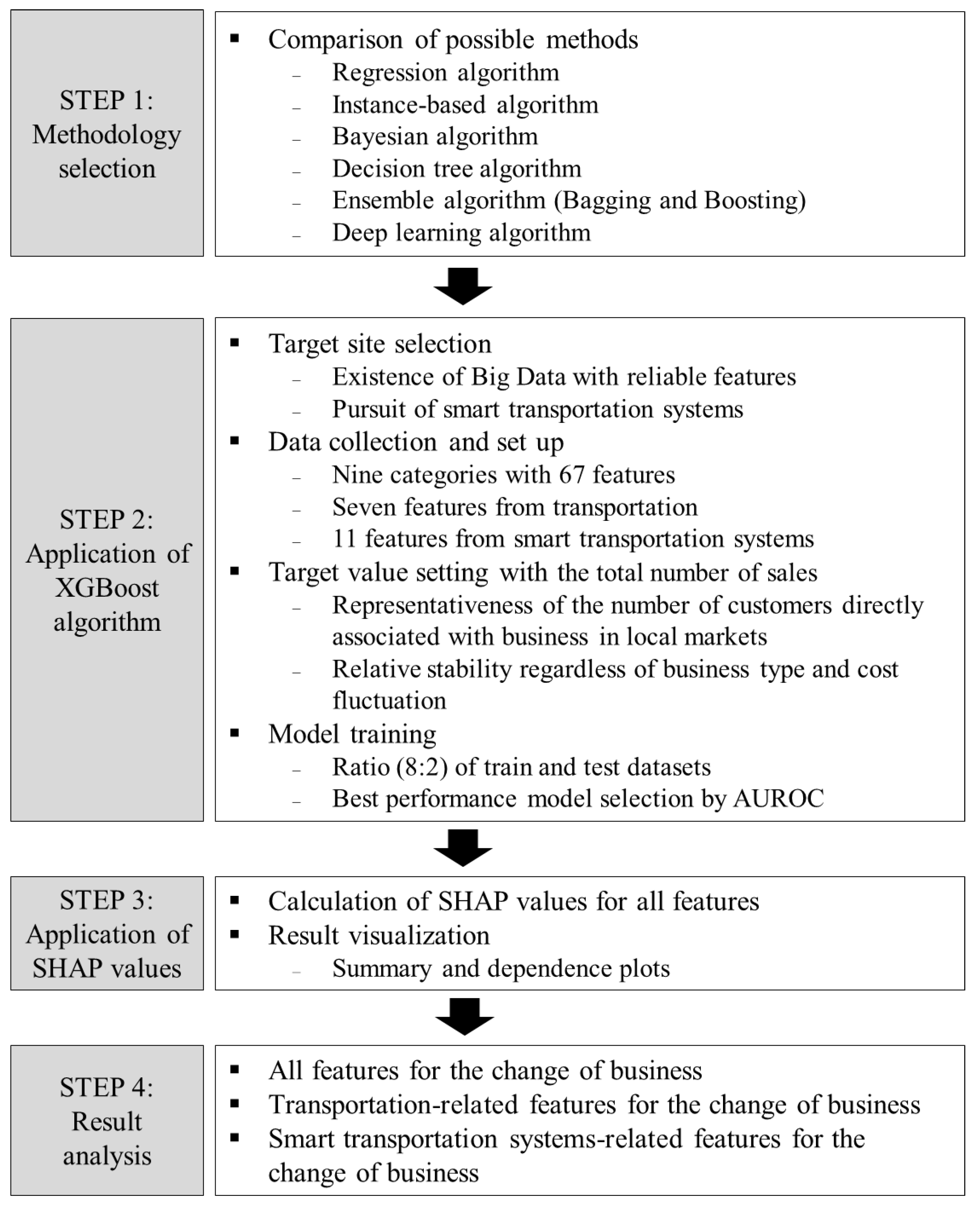
The most suitable methodology needs to be developed in order to overcome limitations found in literature reviews and to achieve the objectives of this research. Figure 1 provides a snapshot of the overall flow of the methodological process used in this research which consists of four steps. After reviewing all possible methods, the most proper method is taken from Ensemble algorithms (Step 1), followed by its applications in Steps 2 and 3 with a target site. Results are eventually interpreted in Step 4 to provide meaningful findings. Details of each step will be described in the methodology and case study sections.

3.1. Comparison of Possible Approaches

To consider a wide range of influential features on economic development in urban areas, this research needs to use methods that are already proven as highly effective and applicable to Big Data sets. At the same time, the method should be trustworthy enough to overcome methodological limitations from previous studies while achieving the objectives of this research. Based on the extensive investigation, machine learning methods were chosen as possible approaches for this research. The following table is a set of possible methods that have been widely used in Big Data analysis. Only methods under the category of supervised machine learning are listed in

Table 3. Possible methods for analysis.

Category	Method	Strength	Weakness
Regression algorithm	Linear Regression	Relatively simple, easy to interpret with the weights, and widely used in various domains.	Only able to provide linear relations and limited predictive performance.
	Logistic Regression	Relatively simple, easy to use, and able to give fast classification (including multiclass) results and probabilities.	Not easy to interpret by its multiplicative feature and limited application to non-linear classification.
Instance-based algorithm	Nearest neighbor	Intuitive to implement, and no assumptions for the data structure (nonparametric) and no training step necessary.	High computational complexity, sensitive to irrelevant or redundant features, and feature scaling necessary.
	Support Vector Machine	Applicable to linear and non-linear problems, and no assumptions for the data structure (nonparametric) necessary.	Relatively difficult to use and interpret, computationally expensive, and lacks transparency of the results.
Bayesian algorithm	Naïve Bayes	Efficient with small datasets and multi-category tasks and less sensitive to irrelevant features.	Strong assumption of independent attributes necessary and sensitive to the form of input data.
Decision tree algorithm	Classification and Regression Tree (CART)	Relatively simple to capture interactions of features and insensitive to the distribution of predictor variables (nonparametric).	Not very stable with small variations and can split only by one variable.
Ensemble algorithm	Bootstrapped Aggregation (Bagging)	Able to reduce variances, high prediction accuracy, and applicable to regression/classification regardless of types of variables.	Computationally expensive, complex to implement, possible to lose interpretability and to give less precise values by mean predictions.
	Boosting	High prediction accuracy and flexibility, easy to interpret, and applicable to regression/classification regardless of types of variables.	Relatively sensitive to irrelevant features, computationally expensive, careful parameter tuning necessary.
Deep learning algorithm	Artificial Neural Network	Good for complicated datasets and able to implicitly detect complex non-linear relationships, all possible interactions between variables.	Complex to apply, difficult to understand the algorithm, dependent on the quantity of the data and great computational burden.

Sources: [38,39,40,41,42,43,44,45,46].

.

Among the methods mentioned above, interest in ensemble algorithms is growing to identify the interactions among features [47,48,49], which is of major interest to this research. Note that although both methods (i.e., Bagging and Boosting) present increased accuracy, there are noticeable differences that need to be considered to determine the final methodology. In principle, both use several models (learners) by using the average to reach the final decision; however, Bagging uses an equally weighed average while Boosting uses a weighted average (better performance with variable interactions). Also, in terms of reducing variance for higher stability, Boosting reduces bias and often outperforms other machine learning methods e.g., [50,51]. Boosting refers to “a general and provably effective method of producing a very accurate prediction rule by combining rough and moderately inaccurate rules of thumb” [52]. Basically, Boosting attempts to convert weak learners to strong learners by training weak learners sequentially (adjusting the weights of weak learners), thereby improving the model predictions. Therefore, to identify influential transportation features from various datasets in this research, Boosting could be the suitable approach by efficiently generating a combined model with lower errors.

Among Boosting techniques (e.g., adaptive boosting or gradient boosting), the extreme gradient boosting (also called “XGBoost”) was selected, which has been successfully proven by data mining challenges (e.g., Kaggle competitions [53]) and by recent studies in other fields e.g., [47,48,49].

3.2. Theoretical Details of XGBoost and SHAP (SHapley Additive exPlanation)

XGBoost was originally created from the concept of gradient boosting presented by Friedman [54] and was developed very recently by Chen and Guestrin [53]. The basic principle of gradient boosting is a straightforward method to build a new model in a gradient direction of the residual errors in order to minimize the loss function which is generated at each iteration. In particular, XGBoost shows its superiority in terms of scalability, parallelization, optimization, and accuracy. The summary of the algorithm is presented here, but more detailed explanations of the XGBoost algorithm can be referred to in Chen and Guestrin [53].

Let a given dataset be $D=\left\{\left(x_i,y_i\right)\right\}\left(\left|D\right|=n,x_i\in R^m,y_i\in R\right)$ with $n$ examples and $m$ features. Equation (1) represents a prediction output function which uses $K$ additive functions.

$${ŷ}_i=\varnothing \left(x_i\right)={{\displaystyle \sum }}_{k=1}^K{f}_k\left(x_i\right),f_k\in \mathcal{F}$$

(1)

where $F=\left\{f\left(x\right)=w_q\left(x\right)\right\}(q:R^m\to T,w\in R^T$)

$K$: number of trees

$f$: tree function in the functional space $F$

$w$: vector of scores in the leaves (weight)

$q$: structure of each tree

$T$: number of leaves in the tree

The objective function to be optimized is given by Equation (2) which can compromise the bias-variance tradeoff to achieve between model performance and operation speed.

$$\mathcal{L}\left(\varnothing \right)={\displaystyle \sum }_{i}l({ŷ}_i,y_i)+{\displaystyle \sum }_k\Omega \left(f_k\right)$$

(2)

where $\Omega \left(f\right)=\gamma T+\frac{1}{2}\lambda \Vert w{\Vert }^2$

$l$: loss function

$\Omega$: regularization term

$\gamma$: complexity cost by additional leaf (minimum loss needed to further partition the leaf node)

$\lambda$: regularization parameter

The objective in Equation (2) is optimized by adding a tree at each iteration, which will be Equation (3) at t-th iteration.

$${\mathcal{L}}^{\left(t\right)}={{\displaystyle \sum }}_{i=1}^{n}l(y_i,{ŷ}_i{}^{\left(t-1\right)}+f_t\left(x_i\right))+\Omega \left(f_i\right)$$

(3)

A second order Taylor expansion of the loss function is applied to solve Equation (4) where $g_i={\partial }_{{ŷ}_i{}^{\left(t-1\right)}}l\left(y_i,{ŷ}_i{}^{\left(t-1\right)}\right)$ and $h_i={\partial }_{{ŷ}_i{}^{\left(t-1\right)}}^{2}l\left(y_i,{ŷ}_i{}^{\left(t-1\right)}\right)$.

$${\mathcal{L}}^{\left(t\right)}\simeq {{\displaystyle \sum }}_{i=1}^n[l(y_i,{ŷ}_i{}^{\left(t-1\right)})+g_i{f}_t\left(x_i\right)+\frac{1}{2}{h}_i{f}_t^2\left(x_i\right)]+\Omega \left(f_t\right)$$

(4)

After removing all constant terms, the specific objective function at step $t$ becomes Equation (5).

$${\tilde{\mathcal{L}}}^{\left(t\right)}={{\displaystyle \sum }}_{i=1}^n[g_i{f}_t\left(x_i\right)+\frac{1}{2}{h}_i{f}_t^2\left(x_i\right)]+\Omega \left(f_t\right)$$

(5)

With the definition above, the objective function can be reformulated as Equation (6) where $I_j$ is defined as a group of examples in the j-th leaf in a certain tree structure.

$$\begin{gathered} {\tilde{\mathcal{L}}}^{\left(t\right)}={{\displaystyle \sum }}_{i=1}^n[g_i{f}_t\left(x_i\right)+\frac{1}{2}{h}_i{f}_t^2\left(x_i\right)]+\gamma T+\frac{1}{2}\lambda {\displaystyle \sum }_{j=1}^T{w}_j^2= \\ {\displaystyle \sum }_{j=1}^T[\left({\displaystyle \sum }_{i\in I_j}{g}_i\right)w_j+\frac{1}{2}\left({\displaystyle \sum }_{i\in I_j}{h}_i+\lambda \right)w_j^2]+\gamma \end{gathered}$$

(6)

From Equation (6), when the tree generates the same weights for the examples in one leaf, the optimal weights can be defined as $w_j^{*}$ and the corresponding optimal value will be ${\tilde{L}}^{\left(t\right)}$ where $q$ denotes a particular tree structure.

$$w_j^{*}=-\frac{{{\displaystyle \sum }}_{i\in I_j}{g}_i}{{{\displaystyle \sum }}_{i\in I_j}{h}_i+\lambda }$$

(7)

$${\tilde{\mathcal{L}}}^{\left(t\right)}\left(q\right)=-\frac{1}{2}{\displaystyle \sum }_{j=1}^T\frac{{({{\displaystyle \sum }}_{i\in I_j}{g}_i)}^2}{{{\displaystyle \sum }}_{i\in I_j}{h}_i+\lambda }+\gamma$$

(8)

To find an optimal split of the tree, Equation (8) plays as an evaluation criterion. The algorithm finds the optimal value greedily by avoiding enumeration of all possible tree structures ($q$). Instead, the algorithm starts splitting from a single leaf into two leaves according to Equation (8). To this end, a loss reduction by the split can be calculated by Equation (9), where $I_L$ and $I_R$ denote the left and right groups of examples, respectively, after splitting.

$${\mathcal{L}}_{split}=\frac{1}{2}\left[\frac{{({{\displaystyle \sum }}_{i\in I_L}{g}_i)}^2}{{{\displaystyle \sum }}_{i\in I_L}{h}_i+\lambda }+\frac{{({{\displaystyle \sum }}_{i\in I_R}{g}_i)}^2}{{{\displaystyle \sum }}_{i\in I_R}{h}_i+\lambda }-\frac{{({{\displaystyle \sum }}_{i\in I}{g}_i)}^2}{{{\displaystyle \sum }}_{i\in I}{h}_i+\lambda }\right]-\gamma$$

(9)

In principle, the best split is to maximize the value of the loss reduction (i.e., the gain is smaller than $\gamma$). After the split process is completed, the leaf values are assigned by Equation (7) to produce the final output.

One of the difficulties of using XGBoost is its result interpretation. To address this problem, Lundberg and Lee [55] proposed a unified framework for interpreting predictions, SHAP (SHapley Additive exPlanations), which can generate values for interpreting complex predictive results from machine learning methods. The concept of SHAP is based on classic Shapley values from a game theory that distributes the total gain or payoff among features according to their relative importance (i.e., magnitude of each contribution) to draw the final output of a game [55,56]. Technically, the Shapley value is the average marginal contribution of a feature value across all possible combinations.

Given that features have different magnitudes of importance to the model’s outputs, that importance can be estimated with the direction (sign) by Shapley value [57]. The positive sign means the positive contribution to the prediction of activity for the final output, whereas the negative sign indicates the opposite contribution to the prediction of activity.

SHAP values are computed by averaging marginal contributions across all possible permutations of a feature set. This is based on the principle of Shapley values to attribute ${\varphi }_i$ values for each feature as in Equation (10) [58].

$${\varphi }_i={\displaystyle \sum }_{S\subseteq N\backslash \left\{i\right\}}\frac{\left|S\right|!\left(M-\left|S\right|-1\right)!}{M!}\left[f_x\left(S\cup \left\{i\right\}\right)-f_x\left(S\right)\right]$$

(10)

where ${\varphi }_i\in R$

$S$: the set of non-zero indexes in $z^{\prime }\in {\left\{0,1\right\}}^M$

$M$: the number of input features

$N$: the number of all input features

$f$: a model

Because of the difficulty in estimating ${\varphi }_i$ for gradient boosting tree models, Lundberg et al. [58] suggested a method for tree SHAP values. This approach was proven as “the only possible consistent, locally accurate method that obeys the missingness property and uses conditional dependence to measure missingness” [55,58]. More details can be found in Lundberg and Lee [55] and Lundberg et al. [58]. With this, SHAP was chosen as a tool to be used for XGBoost in addition to the unique aspect of visualization that summarizes the individual importance of each feature to the prediction of activity. It is noted that the SHAP value of a feature is an average difference between the predictions with and without the feature.

4. Case Study

Based on the methodology proposed, a case study was conducted to reach possible answers to research questions. First, the target site was selected where reliable datasets could be obtained which included necessary variables. Second, data types and features were determined with nine categories that could reflect the objectives of this research. Third, data analysis was performed with the XGBoost algorithm and throughout the process of the target value setting, model training and result visualization with SHAP values. Lastly, results were interpreted from various angles—all features, and transportation- and smart transportation-related features.

4.1. Target Site

The primary objectives of this research are to identify the features affecting economic development in urban areas, including the ones for smart transportation systems. As mentioned above, to incorporate various features, this research adopts the concept of Big Data and relevant techniques, which means specific conditions are required for the case study. Two conditions should be taken into account in this regard: (a) the existence of Big Data with various feasible features, which might affect economic development in urban areas; (b) the pursuit of smart transportation systems in the city agenda. In detail, the target site should maintain an open Big Data platform where specific datasets, particularly related to urban economy, business, transportation, smart transportation, and socio-economics, can be publicly obtained. Also, a variety of smart transportation systems, from traditional to state-of-the-art, should be built in the target city so that a wide range of relevant features can be reflected in the analysis.

Considering such conditions, Seoul in the Republic of Korea was selected as a target site. Seoul is one of the most populous, congested and digital technology-advanced cities in the world and has accurate information data. As of 2019, more than 10 million people were living in Seoul, which spans an area of 30.3 km north-to-south and 34.78 km west-to-east (0.61% of the Republic of Korea) and has 25 autonomous districts (called Gu) and 423 administrative subdistrict units (called Dong) [59]. Although Seoul is regarded as one of the best cities in terms of “mobility and transportation” for facilitating movement through the city and access to public services [60], traffic congestion is still torturing city dwellers (overall average travel time to work/school is 41.12 min, as of September 2019 [61].

In terms of digital technology advancement, the Internet user rate in Seoul was 95% [59]. Further, there was a high penetration rate 80%, [62] of smartphone use in the Republic of Korea, with more than 90% of Seoul citizens using smartphones. A total 2694 locations with 8679 access point installations for free Wi-Fi hotspots existed in 2017 [63]. Smart transportation systems are quite advanced in Seoul, which is regarded as one of the world leaders in this field. For example, more than 9000 buses in Seoul were using real-time management and operations in 2017 [63], as well as more than 35,000 probe taxis, 1181 detectors, 326 variable message signs, and 832 closed-circuit televisions were installed in 2016 [64]. In addition, the Seoul Metropolitan Government maintained an open Big Data platform providing 5198 datasets, 11,906 services, and 4557 open APIs from 70 agencies as of February 2020 [65], which makes it possible to analyze various features to attain the objectives of this research.

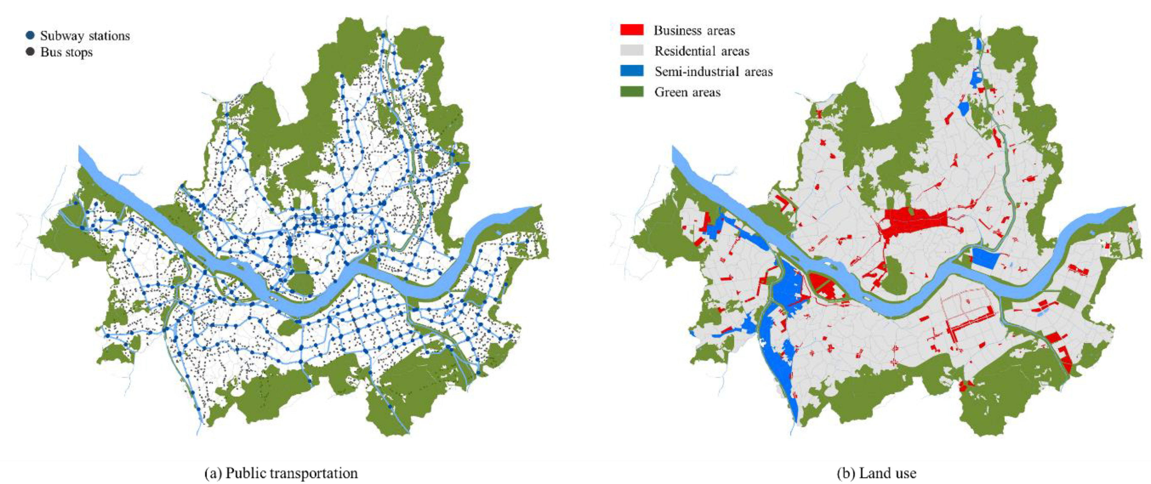
Figure 2 provides a brief overview of public transportation and land use information in the target site.

4.2. Selection of Data Types and Features

A wide range of data was reviewed for the analysis to consider various features in response to the limitations observed in literature reviews. As noted, most previous studies have focused on the relationship between property values and transportation, which can in part be associated with economic development in urban areas. However, it is true that activities associated with business play a critical role in the economic development of urban areas. Further, new technologies have recently been considered a key enabler of industries and economic growth e.g., [68]. More than 140 types of data were reviewed, which were obtained from the Seoul Open Data Plaza, to find the most proper features. The final data set is presented in six groups in

Table 4. Summary of datasets.

Categories	Data	Details	Variables
Classifier	ID	Unique ID for classification	ID
Target value	Change of business	1 = business increase; 0 = others	TGT
Business	Business area code	Distinguishment of business areas	BIZ_AREA_CODE
	Business area type code	A: local business; D: growing business; J: revitalization/neighborhood activation; R: traditional market; U: special tourist zone	BIZ_AREA_TYPE_CODE
	Business type code	Distinguishment of business type	BIZ_TYPE_CODE
Geographical boundary	District code	Autonomous districts	DISTRICT_CODE
	Subdistrict code	Administrative subdistrict units used in business area	SUBDISTRIC_CODE
	Subdistrict code for GIS	Administrative subdistrict units used in GIS	SUBDISTRICT_CODE_GIS
Socio-economic	Resident population per each administrative subdistrict unit	N/A	POPULATION
	Number of employees—manager	N/A	EMPL_POP_MANAGER
	Number of employees—skilled workers	N/A	EMPL_POP_SKILLED
	Number of employees—agriculture, forestry, and fishing workers	N/A	EMPL_POP_AFF
	Number of employees—office workers	N/A	EMPL_POP_OFFICE
	Number of employees—drudge	N/A	EMPL_POP_DRUDGE
	Number of employees—service industry workers	N/A	EMPL_POP_SERVICE
	Number of employees—mechanic and assembly workers	N/A	EMPL_POP_ASM
	Number of employees—professional workers	N/A	EMPL_POP_PRO
	Number of employees—salespersons	N/A	EMPL_POP_SALES
	Number of employees—etc.	N/A	EMPL_POP_ETC
Land value	Average land value per 1 m2 by property (Korean won/m2)	N/A	AVG_LAND_VALUE
Transportation	Number of operating buses per unit area (km2)	N/A	BUS_BY_AREA
	Number of operating buses per 1000 persons	N/A	BUS_BY_PEOPLE
	Number of bus stops per unit area (km2)	N/A	BUS_STOP_BY_AREA
	Number of people per bus stop	N/A	PEOPLE_BY_BUS_ STOP
	Number of subway stations per unit area (km2)	N/A	SUB_STATION_BY_ AREA
	Number of people per subway station	N/A	PEOPLE_BY_SUB_STATION
	Number of parking lots per unit area (km2)	N/A	PARKING_BY_AREA
Smart transportation systems	Number of traffic detectors	N/A	TRAFFIC_DETECTOR
	Number of variable message signs	N/A	VMS
	Number of CCTVs	N/A	CCTV
	Number of traffic CCTVs	N/A	TRAFFIC_CCTV
	Number of vehicle detection systems	N/A	VDS
	Number of lane control systems	N/A	LCS
	Number of public Wi-Fi spots	N/A	PUBLIC_WIFI
	Number of pedestrian light controls	N/A	PEDESTRIAN_LIGHT
	Number of remaining crosswalk time indicator	N/A	RMNG_ INDICATOR
	Number of EV fast-charging stations	N/A	EV_CHARGING
	Ratio of bus information terminals to all bus stops	N/A	BIT_RATIO
Sales	Ratio of sales amount during weekdays	N/A	RATIO_WD_SALES
	Ratio of sales amount during weekends	Exclusive relation to above data	N/A
	Ratio of sales amount by time slots (0 to 6 h)	N/A	RATIO_00TO06_SALES
	Ratio of sales amount by time slots (6 to 11 h)	N/A	RATIO_06TO11_SALES
	Ratio of sales amount by time slots (11 to 14 h)	N/A	RATIO_11TO14_SALES
	Ratio of sales amount by time slots (14 to 17 h)	N/A	RATIO_14TO17_SALES
	Ratio of sales amount by time slots (17 to 21 h)	N/A	RATIO_17TO21_SALES
	Ratio of sales amount by time slots (21 to 24 h)	N/A	RATIO_21TO00_SALES
	Ratio of sales amount by males	N/A	RATIO_MALE_SALES
	Ratio of sales amount by females	Exclusive relation to above data	N/A
	Ratio of sales amount by age groups (10 s)	N/A	RATIO_10S_SALES
	Ratio of sales amount by age groups (20 s)	N/A	RATIO_20S_SALES
	Ratio of sales amount by age groups (30 s)	N/A	RATIO_30S_SALES
	Ratio of sales amount by age groups (40 s)	N/A	RATIO_40S_SALES
	Ratio of sales amount by age groups (50 s)	N/A	RATIO_50S_SALES
	Ratio of sales amount by age groups (over 60 s)	N/A	RATIO_60S_SALES
Floating population	Number of floating males	N/A	PEOPLE_MALE
	Number of floating females	Exclusive relation to above data	N/A
	Number of floating people by age group (10 s)	N/A	PEOPLE_10S
	Number of floating people by age group (20 s)	N/A	PEOPLE_20S
	Number of floating people by age group (30 s)	N/A	PEOPLE_30S
	Number of floating people by age group (40 s)	N/A	PEOPLE_40S
	Number of floating people by age group (50 s)	N/A	PEOPLE_50S
	Number of floating people by age group (over 60 s)	N/A	PEOPLE_60S
	Number of floating people by time slot (0 to 6 h)	N/A	PEOPLE_00TO06
	Number of floating people by time slot (6 to 11 h)	N/A	PEOPLE_06TO11
	Number of floating people by time slot (11 to 14 h)	N/A	PEOPLE_11TO14
	Number of floating people by time slot (14 to 17 h)	N/A	PEOPLE_14TO17
	Number of floating people by time slot (17 to 21 h)	N/A	PEOPLE_17TO21
	Number of floating people by time slot (21 to 24 h)	N/A	PEOPLE_21TO00

Note: This research assumed the sensitivity of data years was not critical for the analysis.

.

As the rise and fall of business is a major consideration when it comes to the success of economic development in urban areas, the target value was set to the change of business and contributing features in socio-economics—land value, transportation, smart transportation systems, sales and floating population—were employed. Resident population and employment were considered two representative socio-economic features. Considering the importance of land values in economic development in urban areas, an average land value per 1 m² in property was employed. Further, as pointed out in literature reviews, previous studies mainly used distance-based accessibility, which could not reflect accurate features of transportation of which various aspects exist. Three dimensions—accessibility, service quality and equity—were accordingly considered, which are major factors when users select their transportation services.

Various features related to smart transportation systems were also incorporated to evaluate their contributions to business in urban areas. A total of 11 features were introduced that encompassed traffic information, traffic operation and management, and electric vehicles. To see the specific magnitude of contributions by sales amount to the target value, ratios of sales amount were used by gender, weekdays, weekends, time-slots, and age groups. As the number of floating people is also an important feature that affects the local business, the number of floating people by gender, age group and time-slots was considered. Last, note that this research assumed the sensitivity of years of data was not critical for the analysis results.

4.3. Data Analysis

4.3.1. Target Value Setting

A specific quantitative measure needed to be decided for business to be used as a target value in the analysis. The total number of sales was chosen as a primary measure for two reasons: (a) its representativeness of the number of customers in local markets which was directly associated with business; and (b) its relative stability compared to other measures, such as prices, which can vary by the type of business and is sensitive to cost fluctuation for raw materials during the study period. Further, the 2017–2019 period was chosen for the analysis, assuming that at least two years were necessary to monitor the impact of selected features on sales. Data that had at least one time of sales per day were considered to increase the reliability of the analysis.

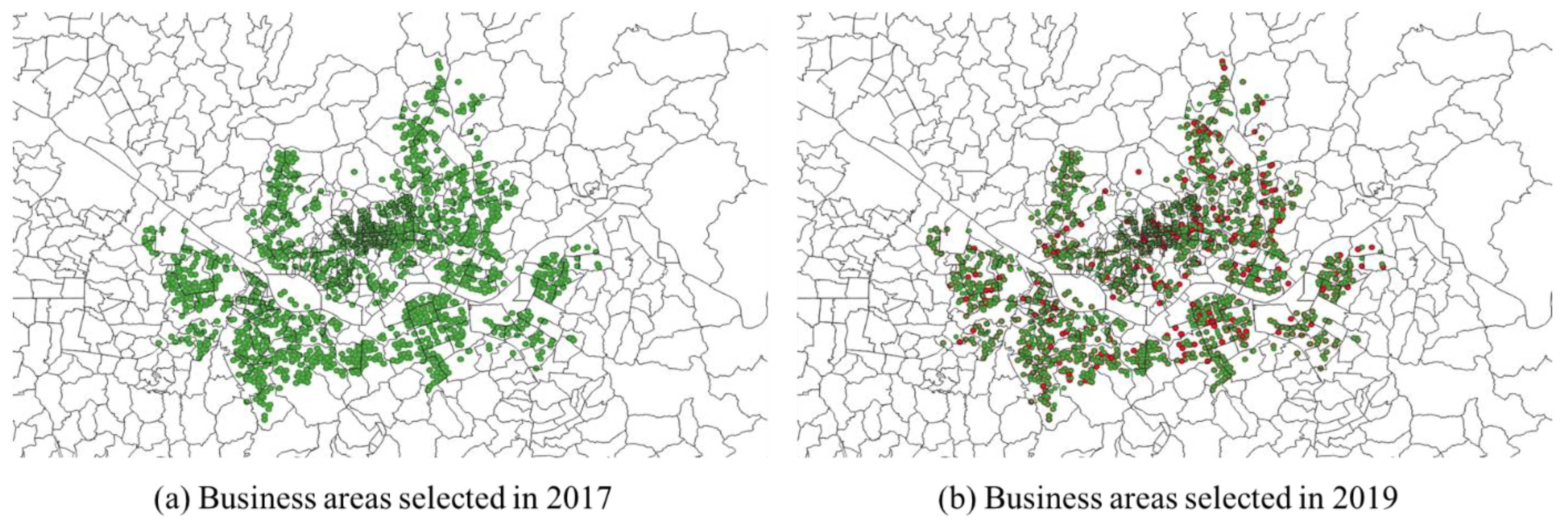
A total of 36,034 specified business areas, generated by a combination of 1493 business area codes and 45 business type codes, were found in 2017, while a total of 31,888 specified business areas were found in 2019, which came under consideration. Among them were 33,645 specified business areas that had more than one time of sales per day during the second quarter of 2017. After comparing with specified business areas in 2019, 29,300 specified business areas remained for further consideration (4345 specified business areas were not found in datasets in 2019). To see the clear influence by selected features, only specified business areas that showed more than a 50% increase in sales during 2017–2019 were used as a target value. Subsequently, it turned out that the rate of being a target value from the refined datasets was 8.8% (2589 out of 29,300 specified business areas). Figure 3 represents all business areas selected in 2017 and in 2019 for the analysis (green dots) and selected areas with increased sales (red dots). It is noted that there were cases that had both increased and decreased sales in one selected area because dots in maps mean areas where businesses were located.

4.3.2. Data Setup, Model Training, and Result Visualization

Data considered in this research were aggregated with different spatial units that needed to be matched up with the codes of business areas. Further, most transportation-related data provided only location information (longitude and latitude coordinates), which were also aggregated by the administrative subdistrict level to match with codes of business areas. GIS software (QGIS) was used to implement the procedures.

After setting up the data, the XGBoost algorithm was applied to train the dataset using Python. Train and test datasets were split in the ratio of 8 to 2 to avoid overfitting. The model performance needs to be monitored simultaneously to draw the most reliable model. An AUROC (the area under the curve of the receiver operation characteristics) was used as a metric to evaluate the model performance. Three parameters were controlled during the training process. First, the number of estimator parameters, which decide the number of boosting rounds, was set as 1500. In addition, the optimal estimators were automatically found by the early stopping option, which stops training a model if the validation score is not improved further. Second, the learning rate parameter, which decides the weight of the previous boosting round, was set as 0.01. Last, the maximum depth parameter, which decides the maximum tree depth, was set to vary from one to nine.

Table 5. The pattern of AUROCs in train and test datasets.

Max Depth	1	2	3	4	5	6	7	8	9
Train dataset	0.6613	0.6867	0.7028	0.7301	0.7801	0.8253	0.8794	0.9195	0.6814
Test dataset	0.6373	0.6425	0.6458	0.6466	0.6522	0.6501	0.6550	0.6506	0.6292
Difference	0.0240	0.0442	0.0570	0.0835	0.1279	0.1752	0.2244	0.2689	0.0522

provides the AUROCs of train and test datasets depending on the max depth. Until eight in the max depth, the AUROC of the train dataset increases. The fluctuation of this metric was noted in the test dataset after five in the max depth, in addition to the increasing difference between the two datasets. The trained model with five of the max depth was accordingly selected as a final model, which can explain clearly the characteristics of both train and test datasets.

As explained above, SHAP values were used to interpret the results from the model which were calculated through Python. Numerical values are provided which can help understand how each feature affects the prediction from datasets. The SHAP package also provides various tools for result interpretation including summary and dependence plots. The summary plot visually shows SHAP values from all features, and the dependence plot provides a specific relationship between SHAP values and feature values in selected features.

4.4. Analysis Results

4.4.1. All Features Analyzed for the Change of Business

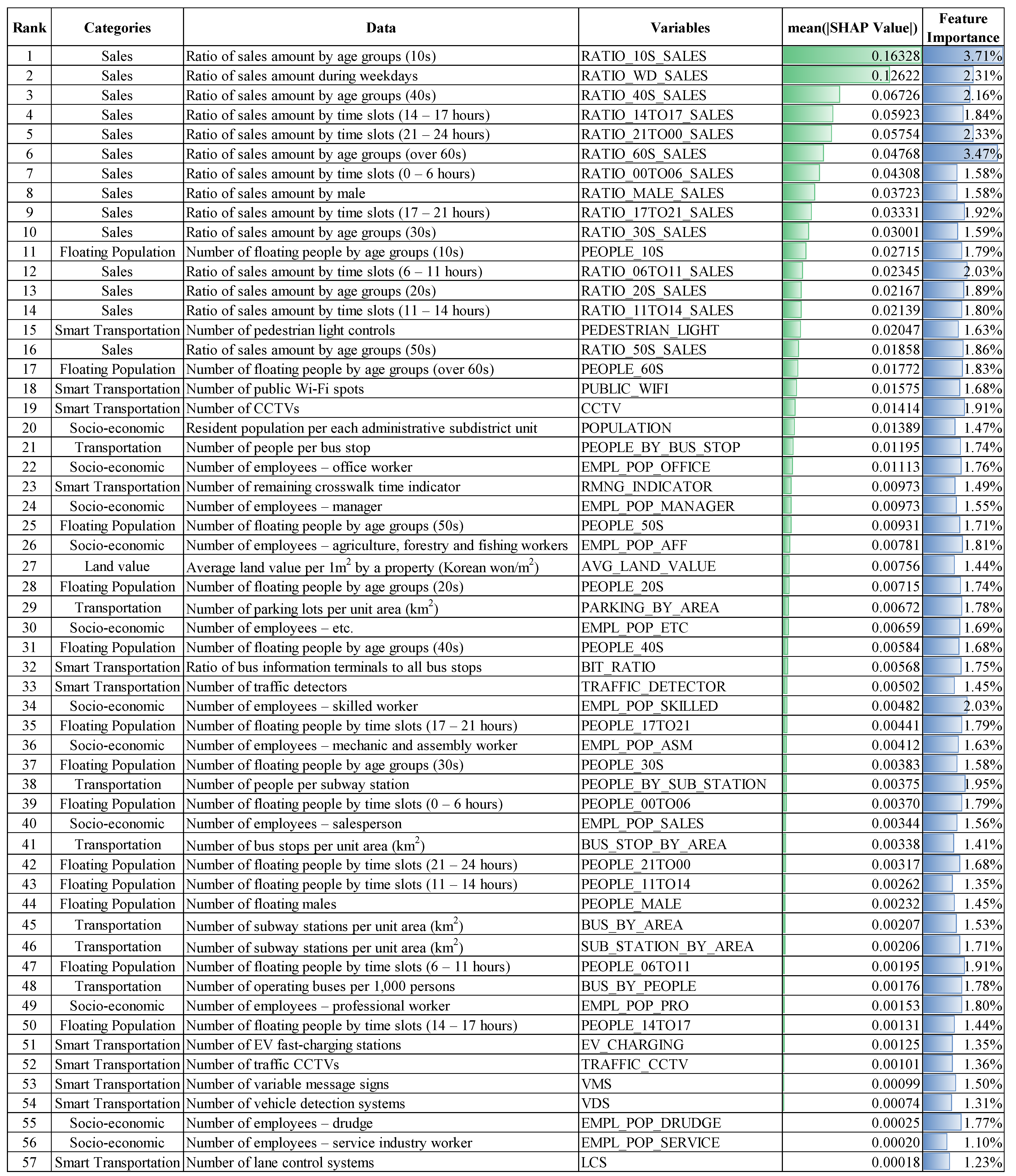
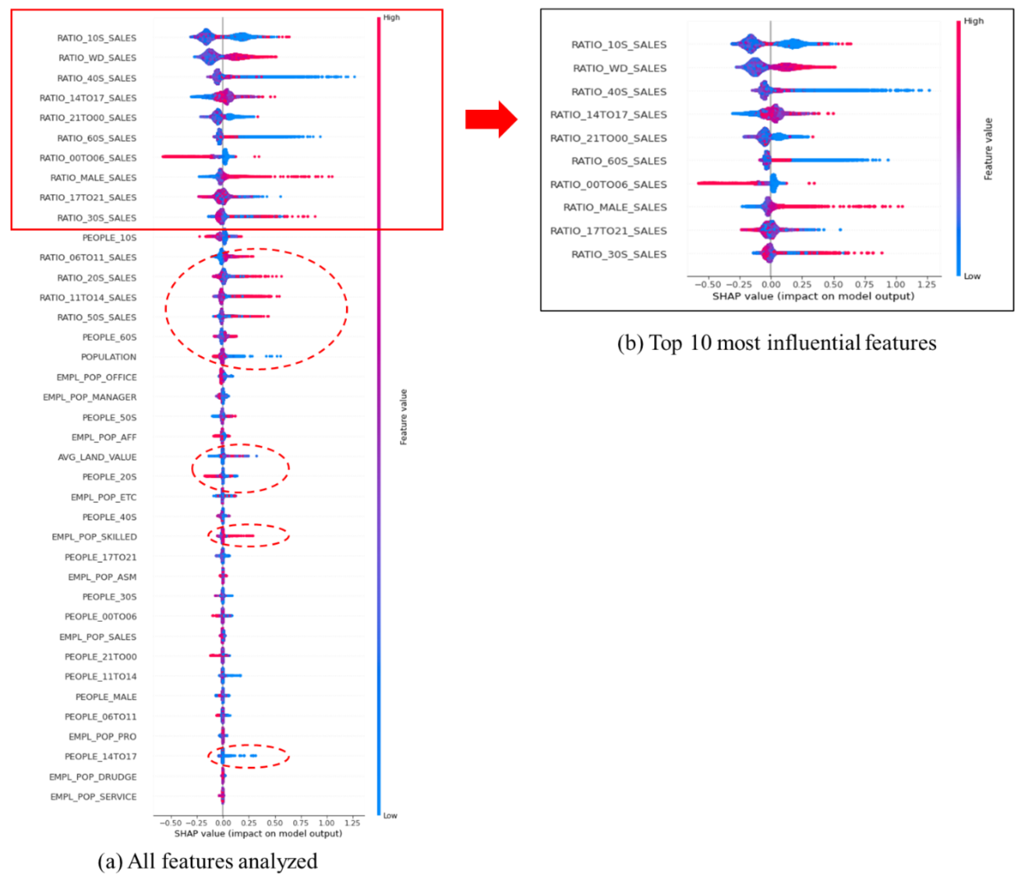
Note that for the intuitive interpretation, the word “contribution” is used in this research which indicates mean absolute SHAP values (an average difference between the predictions with and without the specific feature). According to contributions to the increase in the total number of sales, all features were prioritized as described in Figure 4. In the top 10, all features fall under the sales category, which means sales amount-related features provided significant contributions to business, either positively or negatively. Among them, the ratio of sales amount by 10 s ranked the highest, which produced 0.16328. To a lesser extent, 14 features related to the sales amount, three features related to transportation, two features related to floating population, and one feature related to socio-economics were listed, totaling 20 features. Interestingly, three transportation features are all relevant to smart transportation systems. Here, the feature importance was also presented to give further insight. The feature importance is a relative measure that can be calculated by a portion of the number of frequencies used per each feature, with a total number of frequencies of all features used for the modeling process.

Looking into the average values of contributions to business, features in the sales category showed the largest as 0.05357 among the socio-economics, floating population and sales categories, while features in the other two categories have equal values of 0.00696. The average contribution in the sales category is around 7.7 times larger than the other two categories.

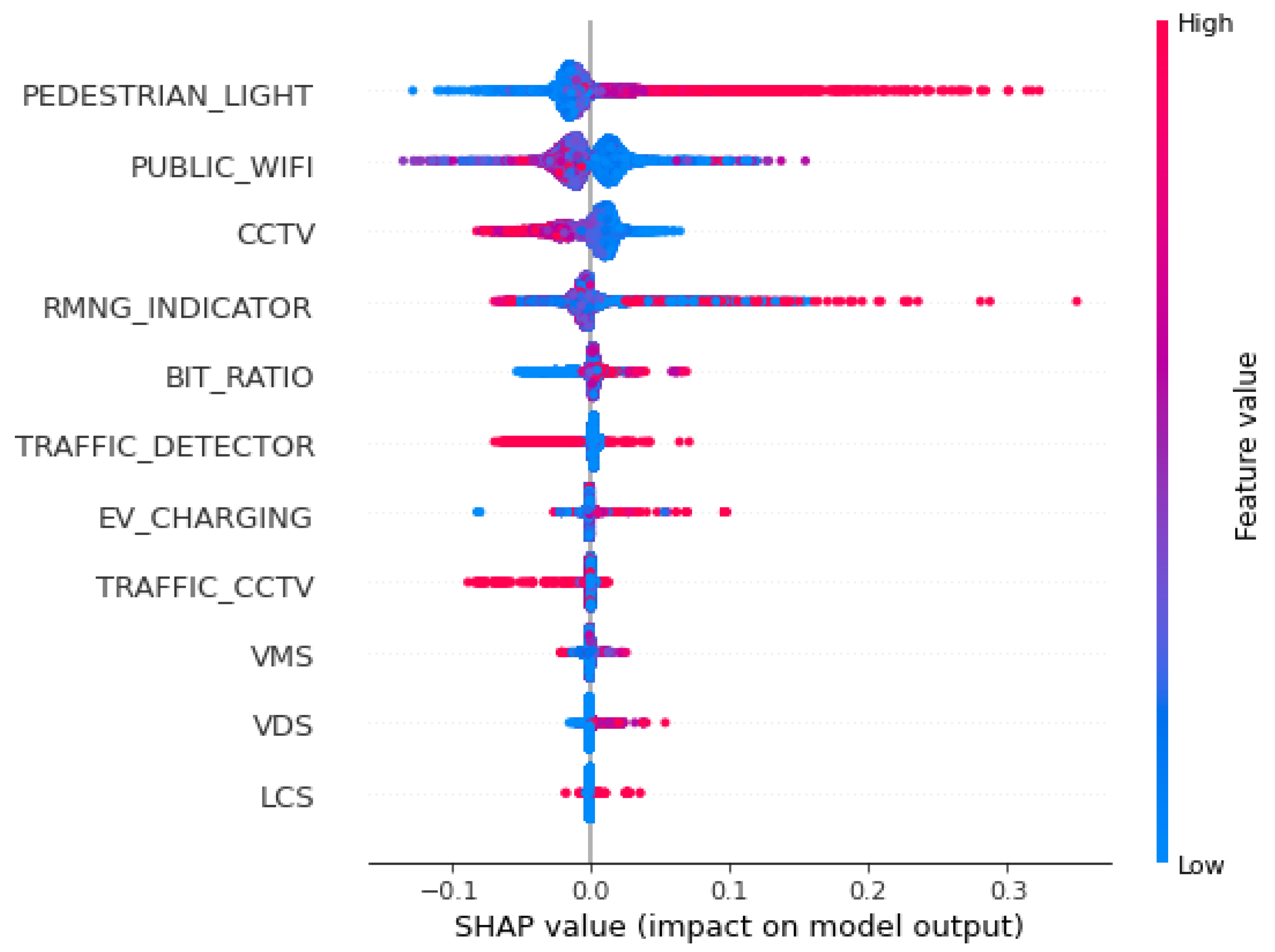
The summary plot is presented in Figure 5 which brings all features to a single plot in the rank order with SHAP values. Each dot represents a single data point, and the color of each dot means the responding value to a feature from low to high. The summary plot gives a sense of the distribution of SHAP values per feature by offering indications of the relationship between the value of a feature and the impact on the prediction (output from the model).

In the top 10 features, the ratio of the sales amount by males during weekdays and by age group (30 s) showed positive contributions to business. This means that activities by males in the 30 s age group during weekdays might relatively affect the rise of business in a target site. To a lesser extent, the ratio of sales amount between 6 and 14 h and by age groups (20 s and 50 s), and the number of employed skilled workers contributed positively to business. It is likely that the core hours to boost business would be from 6 to 14 h, which might accord with workers’ office hours, and stores would be in these areas with the highest number of employees of skilled workers. Interestingly, the resident population and the ratio of sales amount between 14 and 17 h contributed negatively to business. Given that the greater residential population might exist in residential areas where business activities are relatively fewer, increasing the residential population could bring negative contributions to business. Activities during 14 to 17 h in business areas might not contribute to the rise of business; rather, they might be observed in areas where their business is already declining or is relatively non-sensitive. A feature for the average land value showed an inconsistent pattern of contributions being observed, both positively and negatively, that had been assumed as a positive feature in previous studies. More details can be explained through dependence plots.

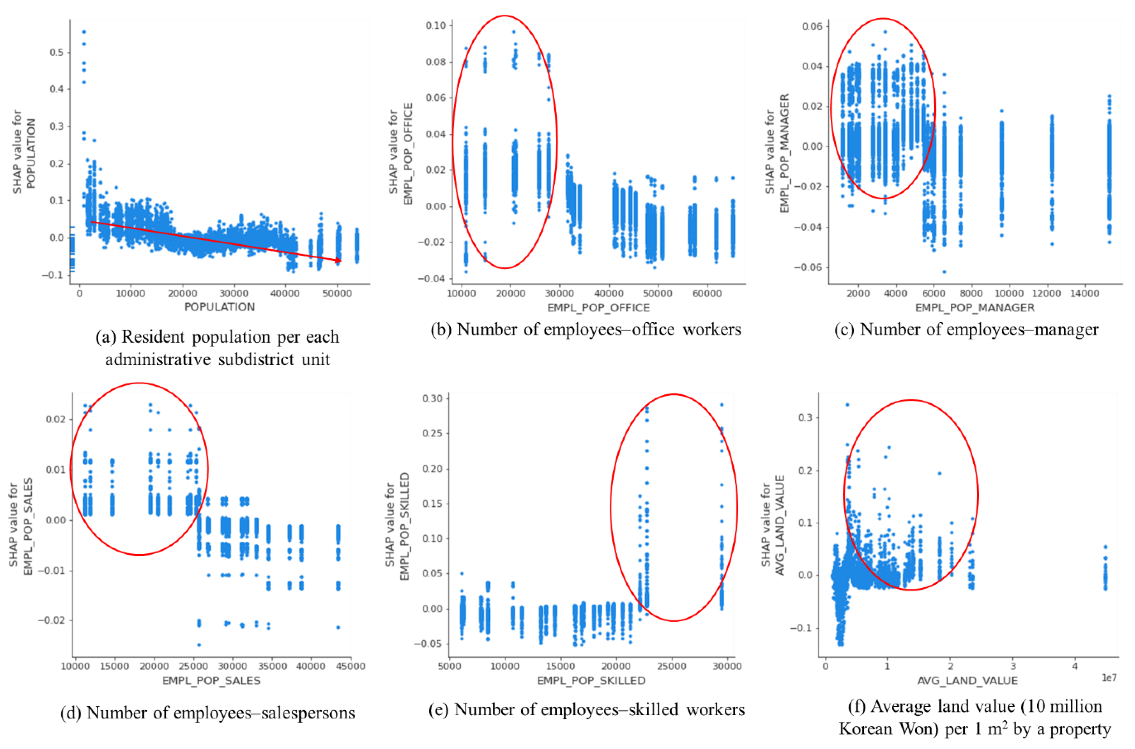
A dependence plot provides a snapshot of distribution by a selected feature. This is depicted by a dot with the value of a feature on the x-axis and the corresponding SHAP value on the y-axis. Only noticeable features were analyzed by category. First, six features were selected from the socio-economic category (Figure 6).

As stated above, the resident population produced a negative contribution to business, which might result from the location of business areas. The number of employed office workers, managers, and salespersons showed strong positive contributions until certain points (around 30,000, 5000, and 25,000 employees, respectively). The rise of business might be contributed by a certain level of the employee numbers of office workers, managers, and salespersons.

On the other hand, the contribution by the employee number of skilled workers significantly increased beyond a certain number, which was around 22,000. Consequently, different patterns were noted within the same category that contributed to the rise of business, which might need customized approaches to increase the number of sales in business areas in a target site.

In terms of the average land value, positive contributions were mostly found after a certain value. This was aligned with the findings to some degree from previous studies regarding the relationship between accessibility and property values e.g., [28,29,69]. However, the magnitude of contribution starts decreasing after the value of 5 million Korean Won, which means a higher land value does not always bring more sales in business. A certain boundary of land values could give the maximum contribution to the rise of business which might affect the choice of locations of business areas. Compared with other studies, Cervero and Kang [30] examined the land market effects by operating median lane bus services in Seoul, which is the same target site of this research. Cervero and Kang [30] revealed that land price premiums were expected within 300 m from bus stops in residential areas, and 150 m in retail and other non-residential areas. Although the approach and research objectives are obviously different, this at least showed that there might be a certain point of land values affected by transportation accessibility which is not always linearly positive. Similarly, many point out that a negative effect on land values exists to some degree depending on geometric accessibility to properties e.g., [69].

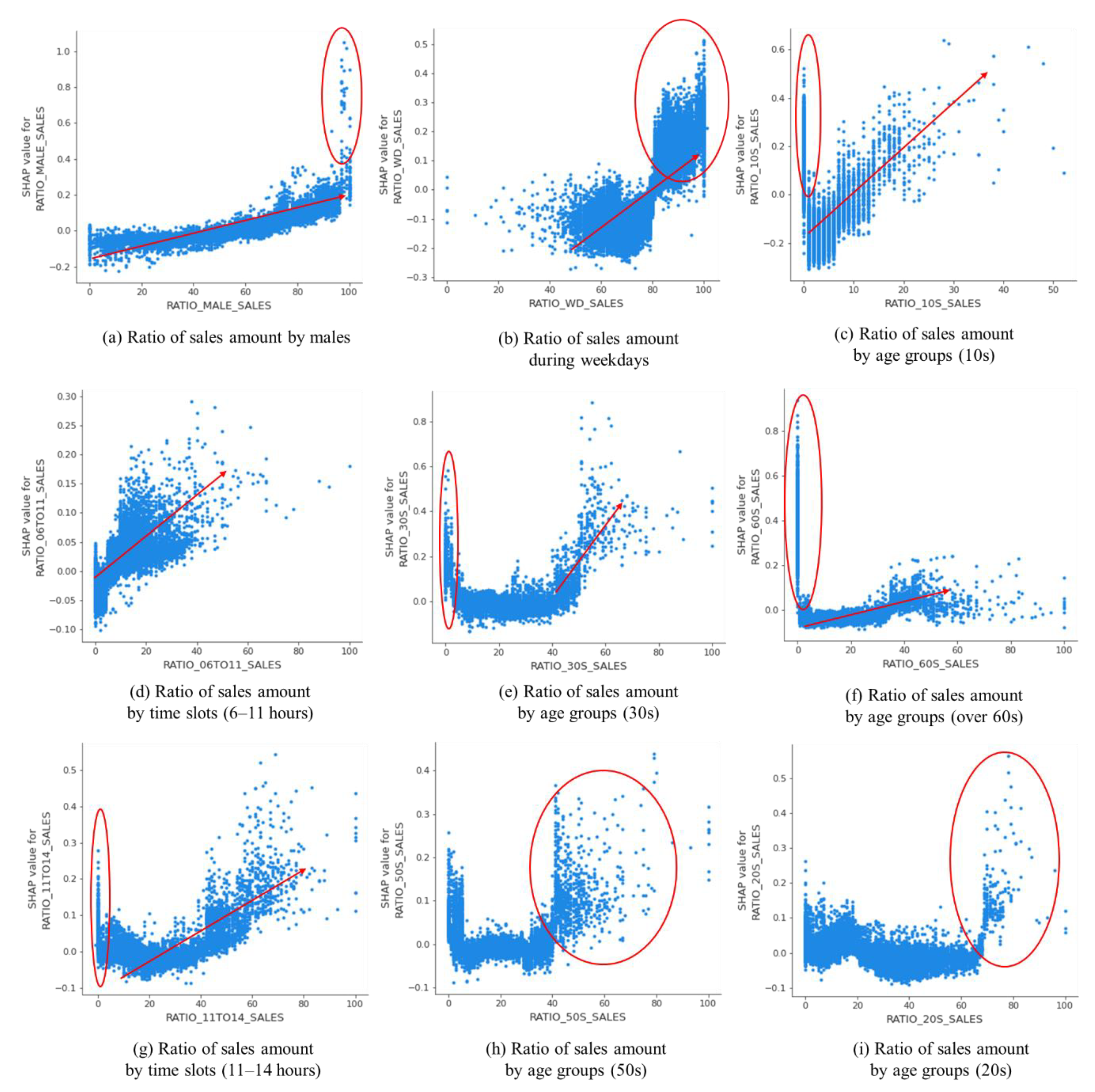
Nine features were chosen from the category of sales (Figure 7).

Features in the sales category presented similar positive patterns. However, some features such as the ratio of sales amount to between 6 and 11 h, by males in the age groups of 20 s and 50 s, and during weekdays exhibited a sudden surge from certain points. This means that the potential of purchasing power in these features (particularly males in the 20 s and 50 s age groups) rises from these points. On the contrary, in some features, such as the ratio of sales, the amount between 11 and 14 h, and by the 10 s, 30 s, and 60 s age groups, SHAP values dropped sharply at zero values and then consistently or inconsistently showed a positive trend. The phenomenon could be explained by the fact that when these features have zero values, other features might contribute strongly in a positive way to the rise of business. Besides, these features would not contribute significantly to the prediction when they have zero values.

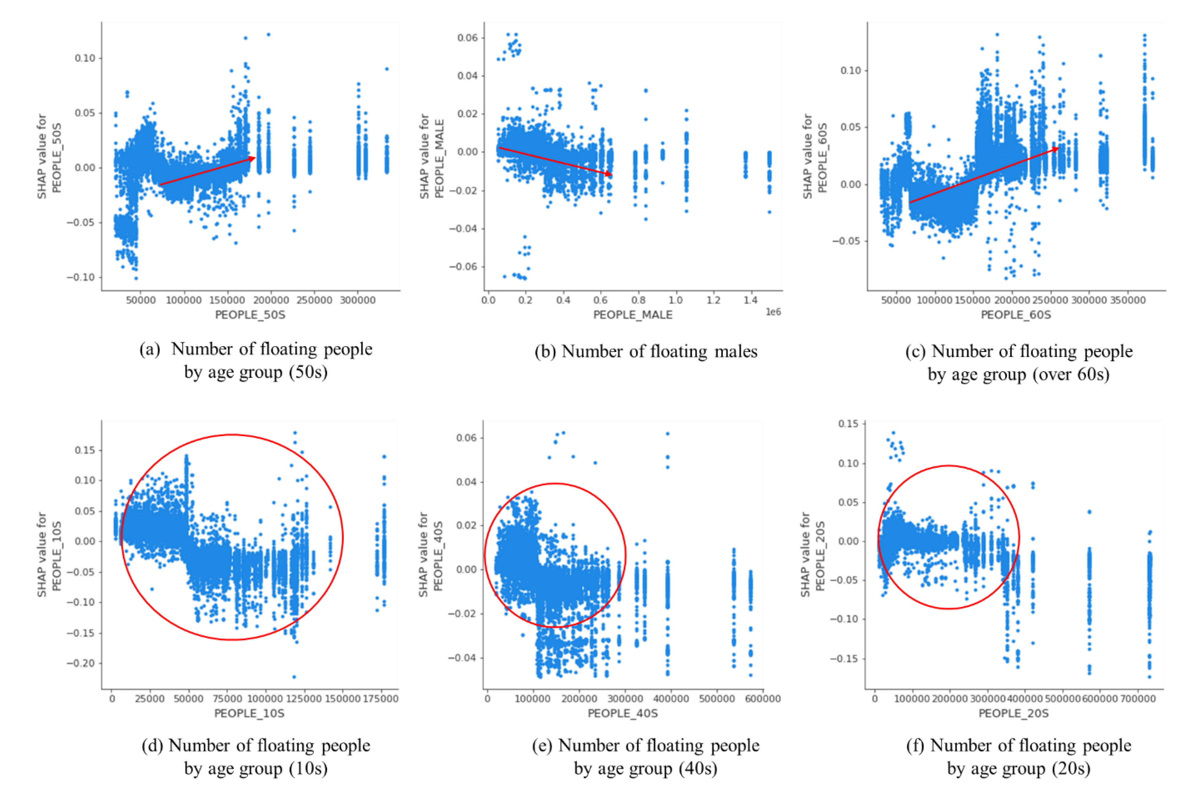
Figure 8 depicts dependence plots for six features in the category of floating population.

Various patterns were found in this category. An increasing pattern of contribution to business was found from the number of floating people in their 60 s while the one for 50 s showed a slight increasing pattern after the value of 70,000. It is reckoned that females might show a positive pattern for contribution to the rise of business. Contrary-wise, more males might bring fewer positive contributions to business. Other features, such as the number of floating people in their 10 s, 20 s, and 40 s, showed strong positive contributions within certain values, which were also observed in other features of the socio-economic and sale categories. That is, after specific values, their contributions remarkably changed from positive to negative. This is because different age groups might bring different patterns of contributions to business.

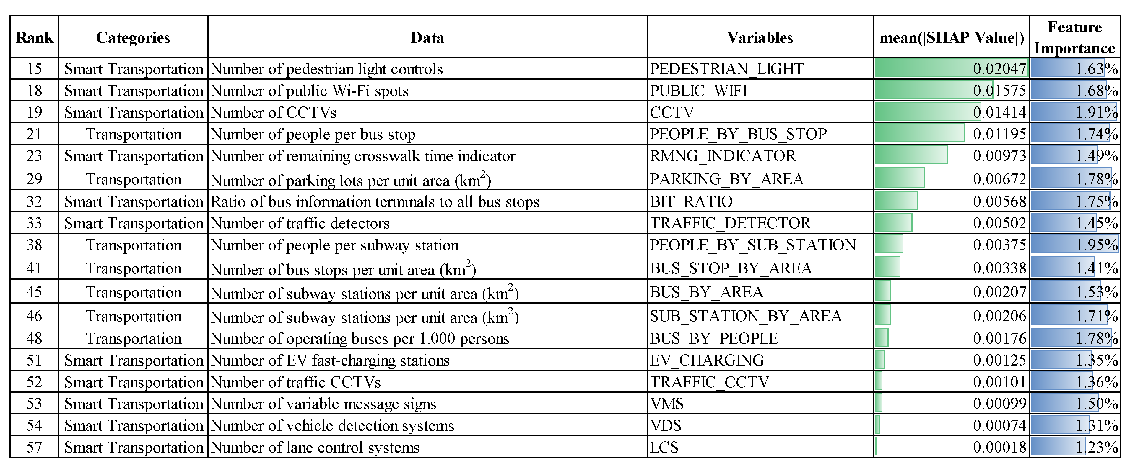
Looking into transportation-related features, including smart transportation systems, 18 features were located from 15 to 57 out of the 57 features considered for the analysis (Figure 9). A total of SHAP values is 0.10666, while other features show 0.91143. It means that total contributions by transportation to the increase in sales in a target site is around 10.5%. Only when considering a total of SHAP values, surprisingly, features related to smart transportation systems show bigger contributions on average than the ones for general transportation (0.00682 vs. 0.00453). Only five features (EV fast-charging stations, traffic CCTVs, variable message signs, vehicle detection systems and lane control systems) from smart transportation systems were ranked as the lowest in terms of the magnitude of contributions. On the other hand, among the five most influential features, pedestrian light controls, public Wi-Fi spots, CCTVs, and remaining crosswalk time indicators were the most influential features for the increase in sales from smart transportation systems. The number of people per bus stop was the only feature that was not relevant to the smart transportation systems ranked in the top five most influential features.

4.4.2. Detailed Findings from Transportation-Related Features

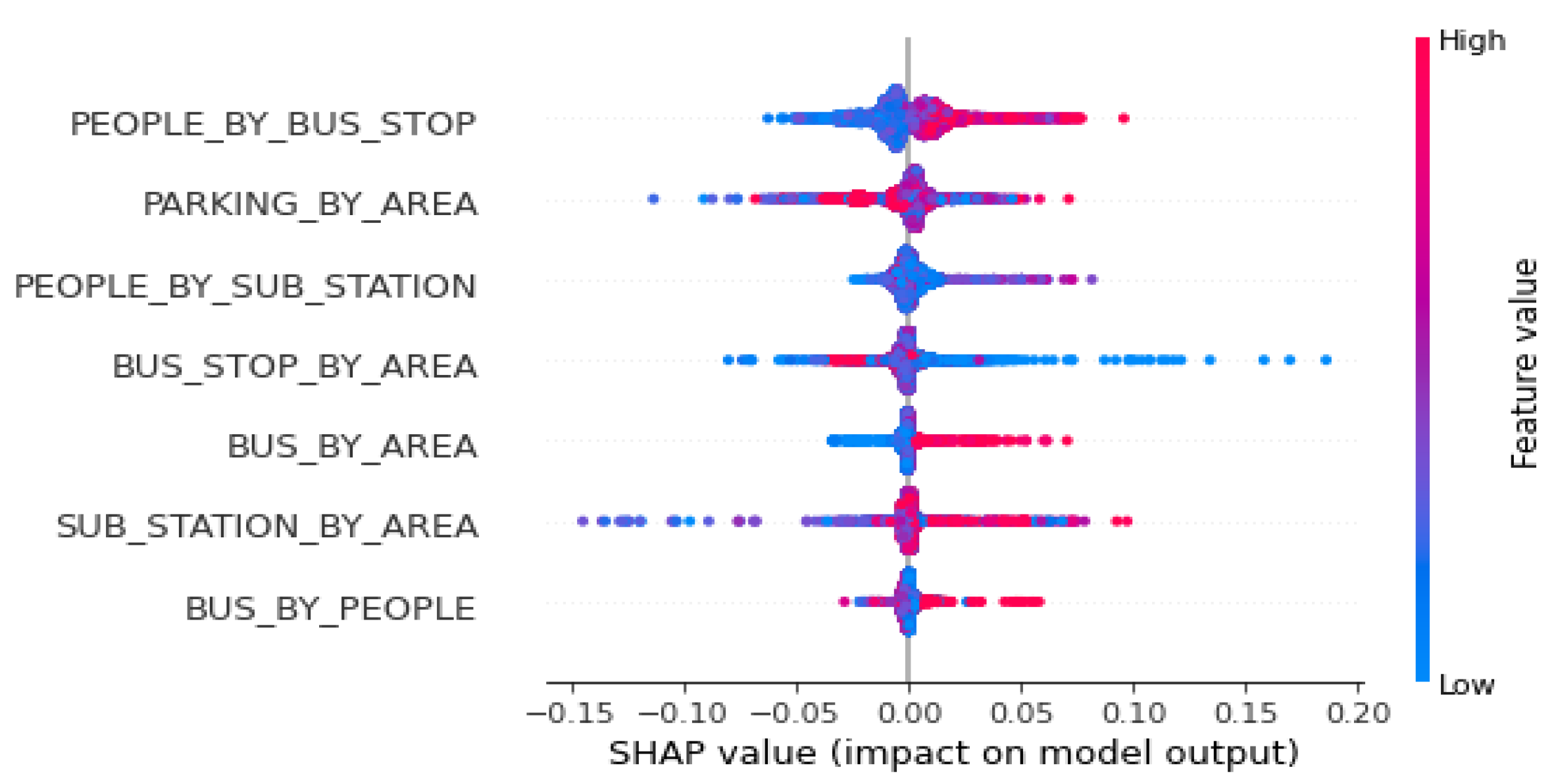
In considering the objectives of this research, the results from transportation-related features were further investigated in order to provide a deeper understanding (Figure 10). A total of seven features were used that might affect business in a target site.

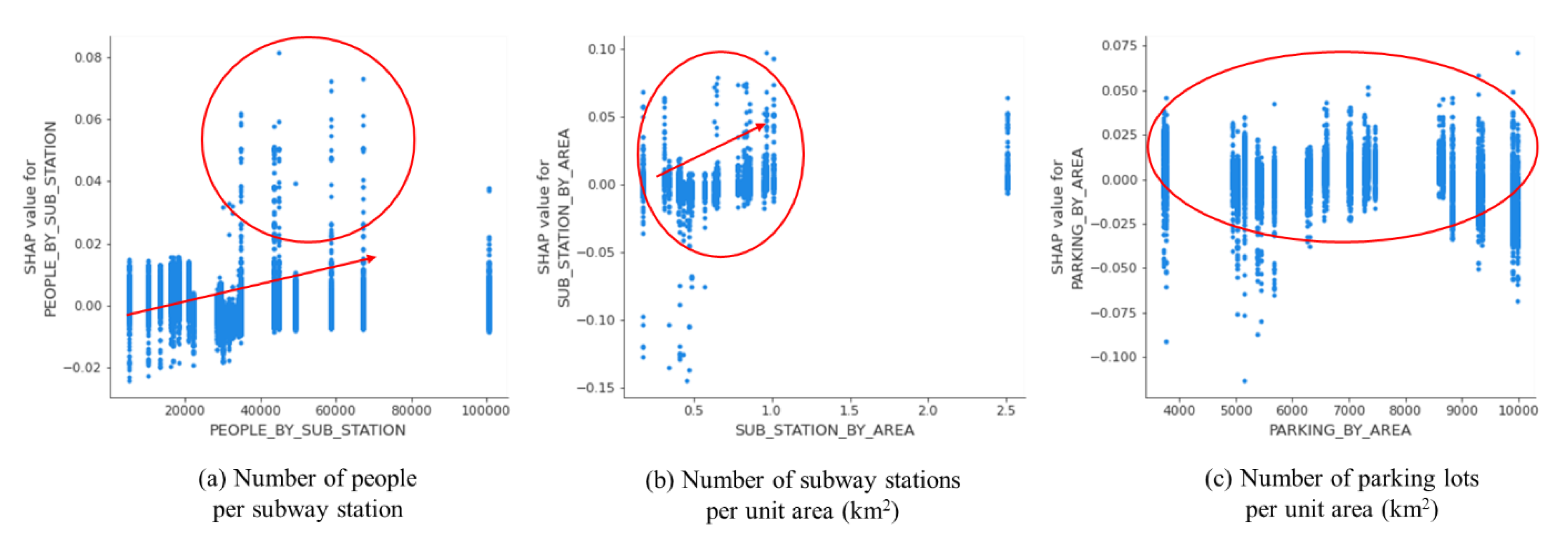
Figure 11 depicts dependence plots for features related to subways and parking facilities.

Considering the critical role of subways in accessibility to business, the number of people per subway station and the number of subway stations per unit area show a positive impact on the increase in sales in a limited way. Specifically, a significant contribution was found for more than 30,000 people per subway station, while a larger number of subway stations per area seems to have higher contributions compared to a smaller number of subway station per area. A relatively positive contribution was also noticed by the number of parking lots per area with an out-of-way sensitivity by the volume of facilities.

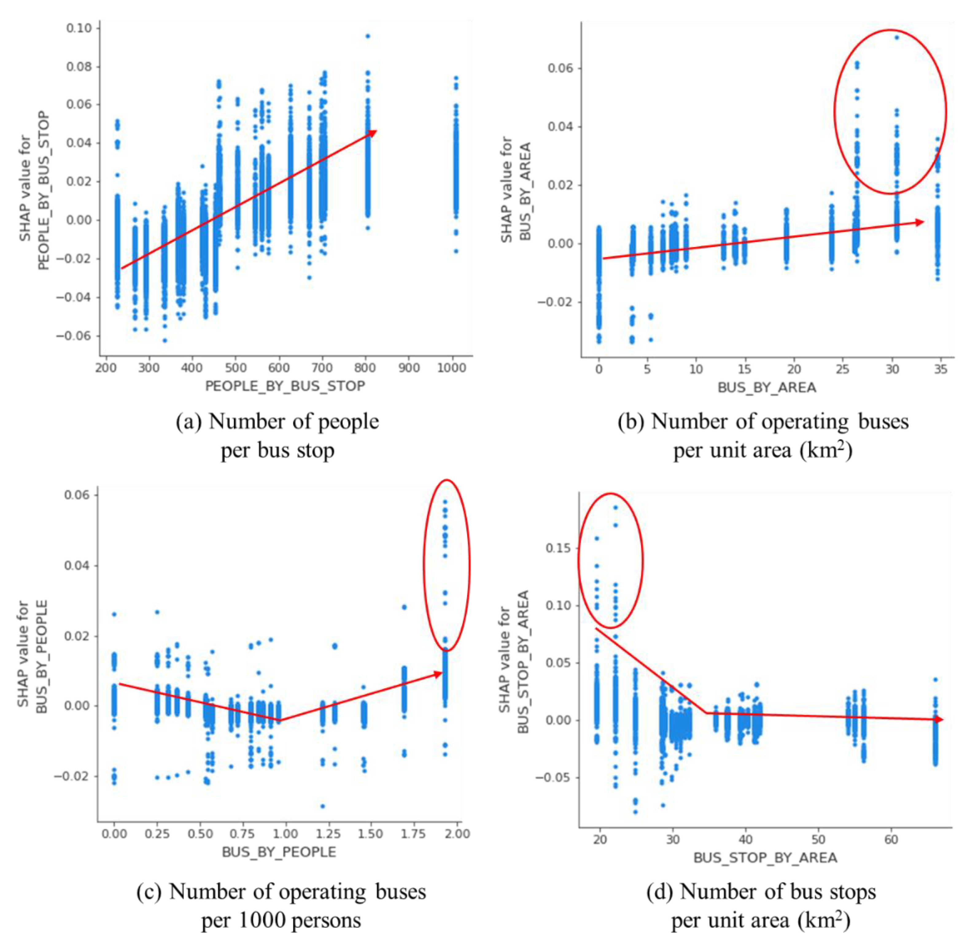
Features related to buses showed more consistent patterns (Figure 12). In detail, people per bus stop showed a positive pattern. The contributions by more than 450 people by bus stop to the increase in sales became significant. Operating buses per unit area also contributed to business especially with more than 25 operating buses per unit area. Operating buses per 1000 persons showed an irregular inclination, but two operating buses per 1000 persons gave noticeable contributions to the increase in sales. It is noted that compared with the features for subways, contributions by bus-related features are more straightforward, meaning that accessibility by buses is more influential in getting customers to visit business areas. Also, SHAP values in the bus-related features are bigger than those in subway-related features.

One atypical phenomenon was found in the number of bus stops per unit area. Fewer contributions were calculated by more bus stops per unit area. In particular, fewer than 25 bus stops per unit area showed the highest contributions, which breaks the mold of typical approaches to the concept of accessibility. Further investigation is required from various angles. However, these business areas might already be in a high-density development where additional bus services are unlikely to be necessary due to high accessibility. Alternatively, they might be in densely built-up areas with mostly narrow passageways between buildings where bus stops are not allowed to be placed.

4.4.3. Detailed Findings from Smart Transportation Systems-Related Features

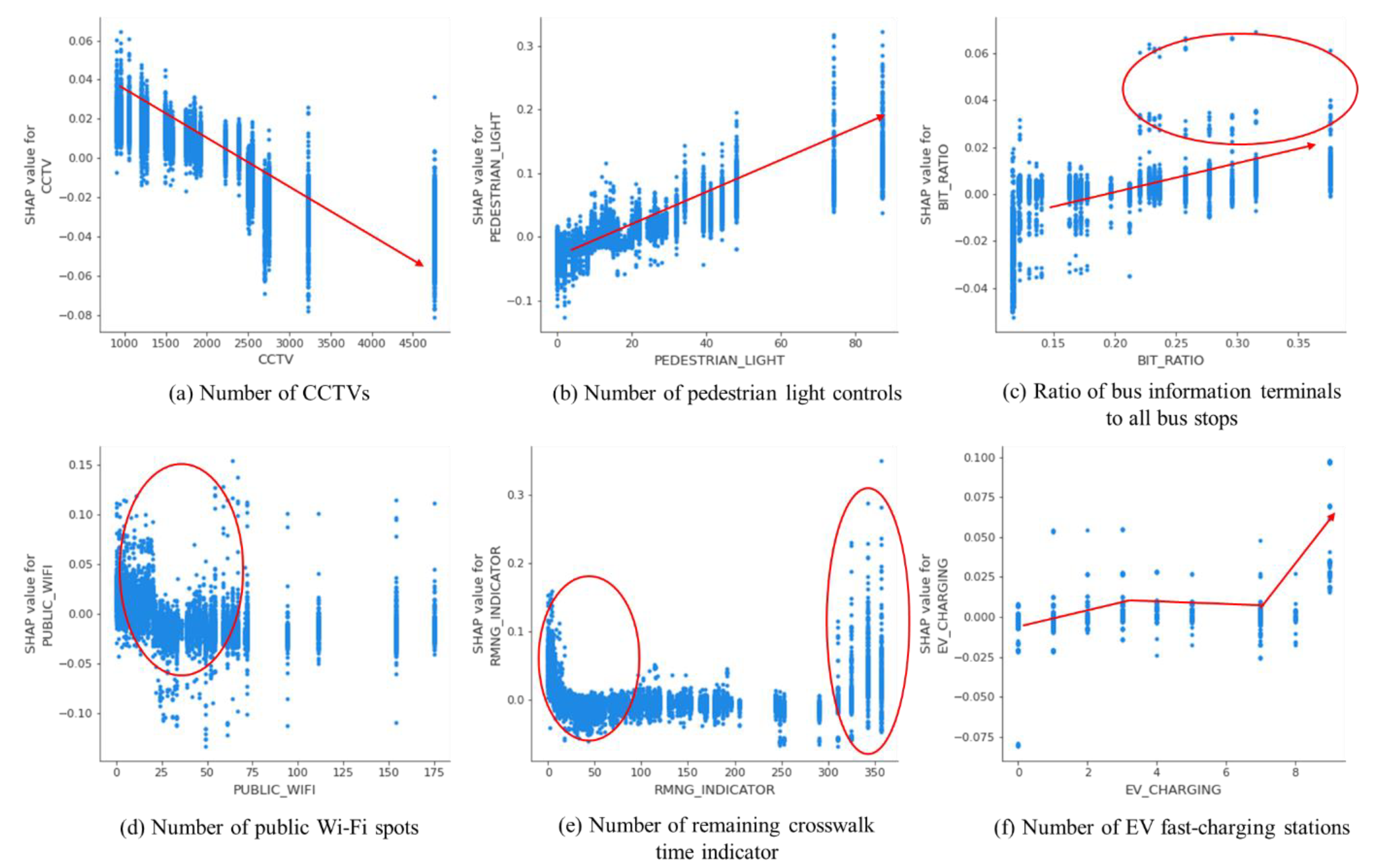
The results for features related to smart transportation systems need to be discussed separately in view of the growing interest in emerging technologies. A couple of features showed meaningful results, as presented in Figure 13.

First of all, a negative pattern was observed when the number of CCTVs increased (Figure 14). With more than 2500 CCTVs per administrative subdistrict unit, the magnitude of negative contributions to the increase in sales became larger (Figure 14). This might result from the fact that CCTVs are usually installed in safety-sensitive areas. In these areas, fewer business activities might occur due to less floating population. Consequently, the increment in sales might be noticed in business areas that are relatively safer with fewer CCTVs.

In contrast, the number of pedestrian light controls and the ratio of bus information terminals to all bus stops showed relatively positive contributions to the increase in sales from certain points. From the customer’s viewpoint, these applications increase convenience, reliability and efficiency, which leads to positive impacts on local business. Although not very strong, positive contributions were found in the ratio of bus information terminals to all bus stops; after the ratio of 0.2, strong contributions appeared in a positive way to increasing sales in a target site.

Interesting results were also found for two features—the number of public Wi-Fi spots and the number of remaining crosswalk time indicators. Fewer public Wi-Fi spots might have a greater effect on increasing sales in business areas. This is not aligned with the general perception that better Wi-Fi connectivity might contribute to the rise of business. However, considering the high penetration rate of the Internet, smartphones, and commercial Wi-Fi spots in a target site, customers might not be very sensitive to the availability of public Wi-Fi spots. Rather, there is a possibility that more public Wi-Fi spots might be installed in lower income-level areas, where robust business activities are not created, to bridge the digital divide within a target site.

Two peaks were found in the dependence plot of the number of remaining crosswalk time indicators. In other words, fewer than 25 and more than 300 indicators per the administrative subdistrict unit showed strong positive contributions to business. The location of business areas, together with the type of business, might be major reasons for this phenomenon. First, traditional markets are usually located in an old town where crosswalks might be fewer or crossing distances might be relatively shorter because of the nature of the town design. Second, the increase in sales might occur more frequently in newly developed business areas where more crosswalk time indicators might be installed to ensure pedestrian safety. Given the fact that the highest contribution was observed in business areas that have more than 300 units, this application might help to increase sales by strengthening traffic safety.

With regard to fast-charging stations for electric vehicles, they are not yet widespread in a target site, but positive contributions by this feature were noted. Interestingly, more than seven stations provided strong positive contributions to the increase in sales in business areas.

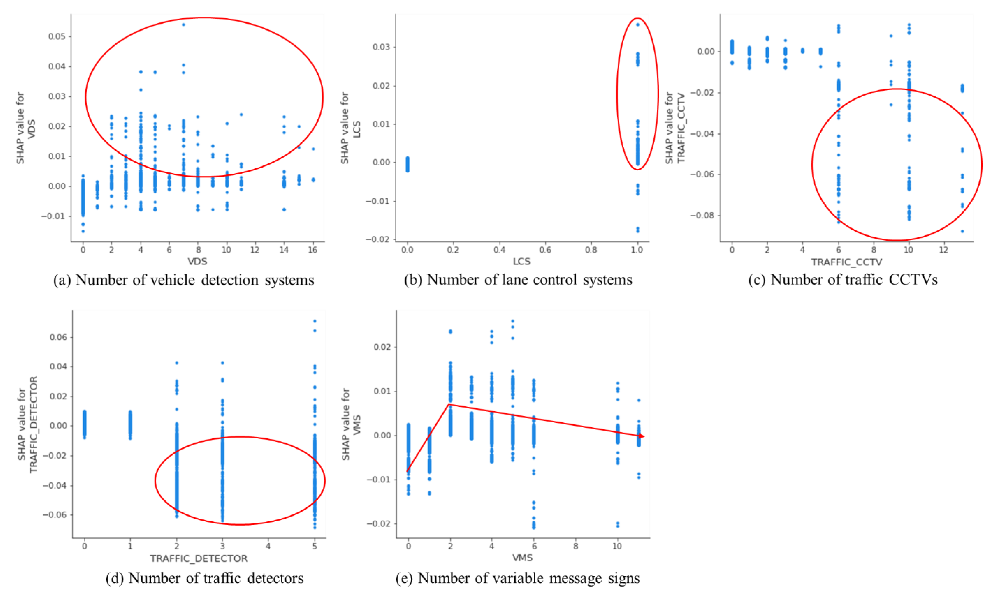
Other features did not show consistent patterns, but some meaningful outcomes could be drawn. Figure 15 depicts dependence plots for five features related to smart transportation systems.

Considering the advantages of vehicle detection systems and lane control systems for optimizing traffic operations, they mostly showed positive contributions to business in an irregular way. However, it was noted that traffic CCTVs and detectors made relatively negative contributions to the increase in sales. This might be because these applications are generally installed on arterial roads, which could produce adverse environmental impacts by heavy traffic, including noise and air pollution. Even if arterial roads could increase accessibility to business areas, such impacts might have a negative influence on business. A similar rationale could be applied to variable message signs, as it showed a negative trend beyond a certain value. Variable message signs disseminate traffic information that could increase customer convenience and efficiency when they visit business areas (positive contributions to business). At the same time, more variable message signs are installed along main roads to disperse the traffic and ensure the efficiency of traffic operations. However, business areas located near main roads could be negatively affected by heavy traffic; thus, from a certain number of variable message signs, they produced relatively negative contributions to the increase in sales in the analysis.

5. Conclusions

Transportation systems have contributed significantly to economic and social activities by connecting people to places in urban areas. However, it is true that transportation-related features, including smart transportation systems, have not been examined for their contributions to economic development in urban areas. Although the rise and fall of business is a good measure for monitoring economic development in urban areas, relevant transportation studies regarding influential features have rarely been carried out in this area. In this regard, efforts have been made to answer the questions that triggered this research. Major achievements from this research are as follows:

• Big Data sets were established through the open Big Data platform. A total of 29,300 specified business areas were considered for the analysis, out of 36,034 in 2017 and 31,888 in 2019;
• More than 140 types of data were reviewed in order to select suitable features from these datasets. Consequently, a total of 67 features were considered from nine categories;
• In particular, diverse features that were not considered in previous studies, i.e., six features in transportation and 11 features in smart transportation systems, were used;
• Cutting-edge machine learning techniques (e.g., XGBoost and SHAP algorithms) were employed to analyze the extent of influential features for business in a target site;
• For each feature, results from the analysis were interpreted with SHAP values in order to understand the impacts on business in each target site.

The findings of the analysis are summarized below and can be referred to for future research and policy directions:

• Features in sales showed the largest contributions to the rise of business. The ratio of sales amount by males during weekdays, by age group (10 s, 30 s, 40 s and over 60 s) and time slots (0–6, 14–17, 17–21 and 21–24 h) were the top 10 features that mostly affected business;
• Unlike previous studies, an inconsistent pattern of contributions from average land value was observed in the rise of business. Given that a certain boundary of land values could provide the maximum contribution, deciding the locations of business areas would affect the findings of business success;
• Unsurprisingly, features related to transportation and smart transportation systems affected business. Relatively larger contributions by smart transportation systems were found in terms of average SHAP values. Four out of the top five transportation-related features were pedestrian light controls, public Wi-Fi spots, CCTVs and remaining crosswalk time indicators, which were relevant to smart transportation systems;
• Fewer CCTVs and public Wi-Fi spots might generate more sales in business, which would be against general perceptions. However, due to the advantages of convenience, efficiency, and reliability, pedestrian light controls generally showed positive effects, whereas remaining crosswalk time indicators had two peaks of highest positive contributions to the resulting increase in business;
• Transportation accessibility is important, but this does not always provide consistent contributions to business. For example, bus-related features showed more influence on business compared to subways. In addition, fewer numbers of bus stops per unit area produced more contributions to the increase in business. This might be the result of the development of business areas where additional bus services were not necessary, or bus stops were not allowed to be added;
• Under the limited deployment of fast-charging stations for electric vehicles, the possibility was shown that this could provide a positive contribution to business. Inconsistent patterns were found for traffic CCTVs, detectors, and variable message signs, which will be noted for further investigations.

All in all, considering the various patterns of contributions from transportation-related features, it can be concluded that: (a) smart transportation systems obviously affect the increase in sales in business; (b) even with the same feature(s), the magnitude and direction of contributions are varied; and (c) some features (e.g., public Wi-Fi spots, remaining crosswalk time indicators, traffic CCTVs, detectors, and variable message signs) showed unconventional results.

These findings can be of use for stakeholders to make relevant policies. In detail, first, town planning authorities can refer to the findings to understand the value of transportation and smart transportation-related features when they design business areas and land uses. Second, transportation planners can prioritize the installation of smart transportation facilities in business areas considering their comparative contributions to economic development in urban areas. Given that different impacts of accessibility by subways and bus stops were noticed, transportation planners can also consider making more efficient transportation networks through customized policies. As fast-charging stations for electric vehicles showed a positive contribution to business, transportation and local authorities can consider it as additional benefits for wider deployment of environmentally friendly transportation modes. Third, business developers might be interested in the results because detailed features in sales were analyzed and the magnitude of average land values to affect business success was identified. This type of information would be an asset to the private sector when they develop the business.

Despite meaningful contributions, a couple of limitations were also found that can guide the future direction of research. For example, although many variables were already considered for the analysis, there are more variables to be considered from smart transportation systems. Features related to shared mobility (e.g., carsharing, ridesharing, bikes-haring, or e-scooter sharing) and/or demand-responsive transportation are a few examples. Second, the level of aggregation units and the point of time for data collection were different for each dataset; thus, this research presumed that the sensitivity of data years was not critical. Yet, if possible, the level of aggregation units and the point of time for data collection need to be aligned for more reliable results. Lastly, as aforementioned, some findings from the analysis did not concur with the general perception from previous transportation studies. Further investigation can be conducted with other external factors to identify details of contributions by features of public Wi-Fi spots, remaining crosswalk time indicators, traffic CCTVs, detectors, and variable message signs.

References

- United Nations. DESA1 (Undated) World Urbanization Prospects: The 2018 Revision. Available online: https://population.un.org/wup/Publications/Files/WUP2018-KeyFacts.pdf (accessed on 15 September 2021).
- DESA2 (Undated) The World’s Cities in 2018. Available online: https://www.un.org/en/events/citiesday/assets/pdf/the_worlds_cities_in_2018_data_booklet.pdf (accessed on 15 September 2021).
- Barrionuevo, J.M.; Berrone, P.; Ricart, J.E. Smart cities, sustainable progress. IESE Insight 2012, 14, 50–57. [Google Scholar] [CrossRef]
- Lima, E.G.; Chinelli, C.K.; Guedes, A.L.A.; Vazquez, E.G.; Hammad, A.W.A.; Haddad, A.N.; Soares, C.A.P. Smart and Sustainable Cities: The Main Guidelines of City Statute for Increasing the Intelligence of Brazilian Cities. Sustainability 2020, 12, 1025. [Google Scholar] [CrossRef] [Green Version]
- Peponi, A.; Morgado, P. Smart and Regenerative Urban Growth: A Literature Network Analysis. Int. J. Environ. Res. Public Health 2020, 17, 2463. [Google Scholar] [CrossRef] [PubMed] [Green Version]
- Ristvej, J.; Lacinák, M.; Ondrejka, R. On Smart City and Safe City Concepts. Mob. Netw. Appl. 2020, 25, 836–845. [Google Scholar] [CrossRef] [Green Version]
- Joss, S.; Sengers, F.; Schraven, D.; Caprotti, F.; Dayot, Y. The Smart City as Global Discourse: Storylines and Critical Junctures across 27 Cities. J. Urban Technol. 2019, 26, 3–34. [Google Scholar] [CrossRef] [Green Version]
- Bhatta, B. Causes and consequences of urban growth and sprawl. In Analysis of Urban Growth and Sprawl from Remote Sensing Data; Advances in Geographic Information Science; Springer: Berlin/Heidelberg, Germany, 2010; pp. 17–36. [Google Scholar]
- Rodriguez-Pose, A.; Frick, S. Urban Centration and Economic Growth. VoxEU, Centre for Economic Policy Research (CEPR). 2018. Available online: https://voxeu.org/article/urban-concentration-and-economic-growth (accessed on 15 September 2021).
- Ferrari, L.; Berlingerio, M.; Calabrese, F.; Reades, J. Improving the accessibility of urban transportation networks for people with disabilities. Transp. Res. Part C Emerg. Technol. 2014, 45, 27–40. [Google Scholar] [CrossRef] [Green Version]
- Litman, T.A. Evaluating Accessibility for Transport Planning: Measuring People’s Ability to Reach Desired Services and Activities; Victoria Transport Policy Institute: Victoria, BC, Canada, 2021; Available online: https://www.vtpi.org/access.pdf (accessed on 15 September 2021).
- Polèse, M. Five Principles of Urban Economics. City J. 2013. Available online: https://www.city-journal.org/html/five-principles-urban-economics-13531.html (accessed on 15 September 2021).
- Martin, R. National growth versus spatial equality? A cautionary note on the new ‘trade-off’ thinking in regional policy discourse. Reg. Sci. Policy Pract. 2008, 1, 3–13. [Google Scholar] [CrossRef]
- Henderson, J.V. Urbanization and growth. In Handbook of Economic Growth; Elsevier: North-Holland, The Netherlands, 2005; Volume 1, Part B; pp. 1543–1591. [Google Scholar]
- Duranton, G.; Turner, M.A. Urban Growth and Transportation. Rev. Econ. Stud. 2012, 79, 1407–1440. [Google Scholar] [CrossRef]
- Kox, H.; Rubalcaba, L. Analysing the Contribution of Business Services to European Economic Growth. Bruges European Economic Research Papers 9; European Economic Studies Department, College of Europe: Bruges, Belgium, 2007. [Google Scholar]
- Fan, J.; Han, F.; Liu, H. Challenges of Big Data analysis. Natl. Sci. Rev. 2014, 1, 293–314. [Google Scholar] [CrossRef] [Green Version]
- Honest, N. A Survey of Big Data Analytics. Int. J. Inf. Sci. Tech. 2016, 6, 35–43. [Google Scholar] [CrossRef]
- Brueckner, J.K. Analyzing Third World Urbanization: A Model with Empirical Evidence. Econ. Dev. Cult. Chang. 1990, 38, 587–610. [Google Scholar] [CrossRef]
- Burchfield, M.; Overman, H.G.; Puga, D.; Turner, M.A. Causes of Sprawl: A Portrait from Space. Q. J. Econ. 2006, 121, 587–633. [Google Scholar] [CrossRef]
- Baum-Snow, N.; Kahn, M.E. The effects of new public projects to expand urban rail transit. J. Public Econ. 2000, 77, 241–263. [Google Scholar] [CrossRef]
- Liu, J.; Zhu, M. Analysis of the Factors Influence on Urban Economic Development Based on Interpretative Structural Model. CSISE 2011, 3, 347–351. [Google Scholar] [CrossRef]
- Zhong, H.; Li, W. Rail transit investment and property values: An old tale retold. Transp. Policy 2016, 51, 33–48. [Google Scholar] [CrossRef]
- Pilgram, C.; West, S.E. Fading premiums: The effect of light rail on residential property values in Minneapolis, Minnesota. Reg. Sci. Urban Econ. 2018, 69, 1–10. [Google Scholar] [CrossRef]
- Gallo, M. The Impact of Urban Transit Systems on Property Values: A Model and Some Evidences from the City of Naples. J. Adv. Transp. 2018, 2018, 1767149. [Google Scholar] [CrossRef]
- Li, Z. The impact of metro accessibility on residential property values: An empirical analysis. Res. Transp. Econ. 2018, 70, 52–56. [Google Scholar] [CrossRef]
- Mulley, C.; Ma, L.; Clifton, G.; Yen, B.; Burke, M. Residential property value impacts of proximity to transport infrastructure: An investigation of bus rapid transit and heavy rail networks in Brisbane, Australia. J. Transp. Geogr. 2016, 54, 41–52. [Google Scholar] [CrossRef] [Green Version]
- Zhang, B.; Li, W.; Lownes, N.; Zhang, C. Estimating the Impacts of Proximity to Public Transportation on Residential Property Values: An Empirical Analysis for Hartford and Stamford Areas, Connecticut. ISPRS Int. J. Geo-Inf. 2021, 10, 44. [Google Scholar] [CrossRef]
- Yang, L.; Zhou, J.; Shyr, O.F. Does bus accessibility affect property prices? Cities 2019, 84, 56–65. [Google Scholar] [CrossRef]
- Cervero, R.; Kang, C.D. Bus rapid transit impacts on land uses and land values in Seoul, Korea. Transp. Policy 2011, 18, 102–116. [Google Scholar] [CrossRef] [Green Version]
- Pan, Q.; Pan, H.; Zhang, M.; Zhong, B. Effects of rail transit on residential property values: Comparison study on the rail transit lines in Houston, Texas, and Shanghai, China. Transp. Res. Rec. J. Transp. Res. Board 2014, 2453, 118–127. [Google Scholar] [CrossRef]
- Calvo, J.A.P. The effects of the bus rapid transit infrastructure on the property values in Colombia. Travel Behav. Soc. 2016, 6, 90–99. [Google Scholar] [CrossRef] [Green Version]
- Yan, S.; Delmelle, E.; Duncan, M. The impact of a new light rail system on single-family property values in Charlotte, North Carolina. J. Transp. Land Use 2012, 5, 60–67. [Google Scholar] [CrossRef] [Green Version]
- Mulley, C. Accessibility and Residential Land Value Uplift: Identifying Spatial Variations in the Accessibility Impacts of a Bus Transitway. Urban Stud. 2013, 51, 1707–1724. [Google Scholar] [CrossRef]
- Dubé, J.; Thériault, M.; Des Rosiers, F. Commuter rail accessibility and house values: The case of the Montreal South Shore, Canada, 1992–2009. Transp. Res. Part A Policy Pract. 2013, 54, 49–66. [Google Scholar] [CrossRef]
- Zvavahera, P.; Chigora, F.; Tandi, R. Entrepreneurship: An Engine for Economic Growth. Int. J. Acad. Res. Bus. Soc. Sci. 2018, 8, 55–66. [Google Scholar] [CrossRef]
- Sarkar, S.; Vinay, S.; Raj, R.; Maiti, J.; Mitra, P. Application of optimized machine learning techniques for prediction of occupational accidents. Comput. Oper. Res. 2019, 106, 210–224. [Google Scholar] [CrossRef]
- Juarez-Orozco, L.E.; Martinez-Manzanera, O.; Nesterov, S.V.; Kajander, S.; Knuuti, J. The machine learning horizon in cardiac hybrid imaging. Eur. J. Hybrid Imaging 2018, 2, 15. [Google Scholar] [CrossRef] [Green Version]
- Molnar, C. Interpretable Machine Learning. 2020. Available online: https://christophm.github.io/interpretable-ml-book/ (accessed on 15 September 2021).
- Lewis, R.J. An Introduction to Classification and Regression Tree (CART) Analysis. 2000. Available online: http://citeseerx.ist.psu.edu/viewdoc/download?doi=10.1.1.95.4103&rep=rep1&type=pdf (accessed on 15 September 2021).
- Singh, S.; Gupta, P. Comparative Study ID3, CART and C4.5 Decision Tree algorithm: A survey. Int. J. Adv. Inf. Sci. Technol. 2014, 27, 97–103. [Google Scholar] [CrossRef]
- Imandoust, S.B.; Bolandraftar, M. Application of K-nearest neighbor (KNN) approach for predicting economic events: Theoretical background. Int. J. Eng. Res. Appl. 2013, 3, 605–610. [Google Scholar]
- Auria, L.; Moro, R.A. Support Vector Machines (SVM) as a Technique for Solvency Analysis; Discussion Papers of DIW Berlin 811; DIW Berlin, German Institute for Economic Research: Berlin, Germany, 2008. [Google Scholar] [CrossRef] [Green Version]
- Basheer, I.; Hajmeer, M. Artificial neural networks: Fundamentals, computing, design, and application. J. Microbiol. Methods 2000, 43, 3–31. [Google Scholar] [CrossRef]
- Xhemali, D.; Hinde, C.J.; Stone, R.G. Naïve Bayes vs. Decision Trees vs. Neural Networks in the Classification of Training Web Pages. Int. J. Comput. Sci. Issues 2009, 4, 16–23. [Google Scholar]
- Mohamed, A.E. Comparative study of four supervised machine learning techniques for classification. Int. J. Appl. Sci. Technol. 2017, 7, 5–18. [Google Scholar]
- Guo, J.; Yang, L.; Bie, R.; Yu, J.; Gao, Y.; Shen, Y.; Kos, A. An XGBoost-based physical fitness evaluation model using advanced feature selection and Bayesian hyper-parameter optimization for wearable running monitoring. Comput. Netw. 2019, 151, 166–180. [Google Scholar] [CrossRef]
- Song, K.; Yan, F.; Ding, T.; Gao, L.; Lu, S. A steel property optimization model based on the XGBoost algorithm and improved PSO. Comput. Mater. Sci. 2019, 174, 109472. [Google Scholar] [CrossRef]
- Carmona, P.; Climent, F.; Momparler, A. Predicting failure in the U.S. banking sector: An extreme gradient boosting approach. Int. Rev. Econ. Finance 2019, 61, 304–323. [Google Scholar] [CrossRef]
- Filippi, A.M.; Guneralp, I.; Randall, J. Hyperspectral remote sensing of aboveground biomass on a river meander bend using multivariate adaptive regression splines and stochastic gradient boosting. Remote Sens. Lett. 2014, 5, 432–441. [Google Scholar] [CrossRef]
- Freeman, E.A.; Moisen, G.G.; Coulston, J.W.; Wilson, B.T. Random forests and stochastic gradient boosting for predicting tree canopy cover: Comparing tuning processes and model performance. Can. J. For. Res. 2016, 46, 323–339. [Google Scholar] [CrossRef] [Green Version]
- Schapire, R.E. The Boosting Approach to Machine Learning: An Overview. In Nonlinear Estimation and Classification; Lecture Notes in Statistics; Denison, D.D., Hansen, M.H., Holmes, C.C., Mallick, B., Yu, B., Eds.; Springer: New York, NY, USA, 2003; Volume 171, pp. 149–171. [Google Scholar]
- Chen, T.; Guestrin, C. XGBoost: A Scalable Tree Boosting System. In Proceedings of the 22nd ACM SIGKDD International Conference on Knowledge Discovery and Data Mining, San Francisco, CA, USA, 13–17 August 2016; pp. 785–794. [Google Scholar] [CrossRef] [Green Version]
- Friedman, J.H. Greedy function approximation: A gradient boosting machine. Ann. Stat. 2001, 29, 1189–1232. [Google Scholar] [CrossRef]
- Lundberg, S.M.; Lee, S.-I. A unified approach to interpreting model predictions. arXiv 2017, arXiv:1705.07874. [Google Scholar] [CrossRef]
- Shapley, L. A value for n-Person Games. In Contributions to the Theory of Games II; Princeton University Press: Princeton, NJ, USA, 1953; pp. 307–317. [Google Scholar] [CrossRef]
- Rodríguez-Pérez, R.; Bajorath, J. Interpretation of machine learning models using shapley values: Application to compound potency and multi-target activity predictions. J. Comput. Mol. Des. 2020, 34, 1013–1026. [Google Scholar] [CrossRef]
- Lundberg, S.M.; Erion, G.G.; Lee, S.-I. Consistent individualized feature attribution for Tree Ensembles. arXiv 2019, arXiv:1802.03888. [Google Scholar] [CrossRef]
- Seoul Metropolitan Government. City Overview. 2019. Available online: http://english.seoul.go.kr/seoul-views/meaning-of-seoul/2-location/ (accessed on 15 September 2021).
- IESE Business School. IESE Cities in Motion Index 2018 (ST-471-E); University of Navarra: Barcelona, Spain, 2018; Available online: https://media.iese.edu/research/pdfs/ST-0471-E.pdf (accessed on 15 September 2021).
- Numbeo. Traffic in Seoul, South Korea. 2019. Available online: https://www.numbeo.com/traffic/in/Seoul (accessed on 16 September 2021).
- Statista. Smartphone Penetration Rate as Share of the Population in South Korea from 2015 to 2025. 2019. Available online: https://0-www-statista-com.brum.beds.ac.uk/statistics/321408/smartphone-user-penetration-in-south-korea/ (accessed on 16 September 2021).
- Seoul Metropolitan Government. Seoul’s Policy Sharing Initiative. 2017. Available online: http://susa.or.kr/sites/default/files/resources/%EC%84%9C%EC%9A%B8%EC%8B%9C_%EC%A0%95%EC%B1%85%ED%86%B5%ED%95%A9%EB%B8%8C%EB%A1%9C%EC%8A%88%EC%96%B4_%EC%98%81%EB%AC%B8_%EB%B3%B4%EA%B8%B0%EC%9A%A9.pdf (accessed on 16 September 2021).
- Ko, J.; Shin, L. TOPIS: Seoul’s Intelligent Traffic System (ITS). Seoul Solution. 2014. Available online: https://seoulsolution.kr/en/content/2595 (accessed on 16 September 2021).
- Seoul Open Data Plaza. Seoul Metropolitan Government. 2020. Available online: https://data.seoul.go.kr/ (accessed on 16 September 2021).
- Korea National Spatial Data Infrastructure Portal. Spatial Information Service. Ministry of land, Infrastructure and Transport. 2021. Available online: http://www.nsdi.go.kr/lxportal/?menuno=3085 (accessed on 15 September 2021).
- Korea Public Data Portal. Ministry of the Interior and Safety. 2022. Available online: https://www.data.go.kr/en/index.do (accessed on 6 April 2022).
- Colecchia, A.; Schreyer, P. ICT Investment and Economic Growth in the 1990s: Is the United States a Unique Case? A Comparative Study of Nine OECD Countries. No 2001/7, OECD Science, Technology and Industry Working Papers, OECD Publishing. 2001. Available online: https://EconPapers.repec.org/RePEc:oec:stiaaa:2001/7-en (accessed on 15 September 2021).
- Morales, J.; Flacke, J.; Zevenbergen, J. Modelling residential land values using geographic and geometric accessibility in Guatemala City. Environ. Plan. B Urban Anal. City Sci. 2019, 46, 751–776. [Google Scholar] [CrossRef]
Figure 1.
Overall methodological process for the analysis.
Figure 2.
Public transportation and land use information in Seoul (map data sources: [66,67]). Note: Maps were created by the authors with data sources publicly available.
Figure 3.
Target business areas in 2017 and 2019 (map data source: [66]). Note: Maps were created by the authors with analysis results and a data source publicly available.
Figure 4.
All features in order by mean absolute SHAP values.
Figure 5.
A summary plot for all features with the top 10 most influential features.
Figure 6.
Dependence plots for six features from the socio-economic category.
Figure 7.
Dependence plots for nine features from the sales category.
Figure 8.
Dependence plots for six features from the floating population category.
Figure 9.
Transportation-related features in order by mean absolute SHAP values.
Figure 10.
A summary plot for transportation-related features.
Figure 11.
Dependence plots for features related to subways and parking facilities.
Figure 12.
Dependence plots for features related to bus services.
Figure 13.
A summary plot for smart transportation-related features.
Figure 14.
Dependence plots for features with clear patterns related to smart transportation systems.
Figure 15.
Dependence plots for features with less clear patterns related to smart transportation systems.