
A Novel Community Detection Method of Social Networks for the Well-Being of Urban Public Spaces

1
Department of Software Convergence, Soonchunhyang University, Asan-si 31538, Chungcheongnam-do, Korea
2
School of Computer Science, Shaanxi Normal University, Xi’an 710119, China
3
Institute for Artificial Intelligence and Software, Soonchunhyang University, Asan-si 31538, Chungcheongnam-do, Korea
*
Author to whom correspondence should be addressed.
Land 2022, 11(5), 716; https://0-doi-org.brum.beds.ac.uk/10.3390/land11050716
Submission received: 31 March 2022
/
Revised: 3 May 2022
/
Accepted: 7 May 2022
/
Published: 10 May 2022
(This article belongs to the Special Issue Landscape Based Land Solutions and Big Data)
Abstract
:A third place (public social space) has been proven to be a gathering place for communities of friends on social networks (social media). The regulars at places of worship, cafes, parks, and entertainment can also possibly be friends with those who follow each other on social media, with other non-regulars being social network friends of one of the regulars. Therefore, detecting and analyzing user-friendly communities on social networks can provide references for the layout and construction of urban public spaces. In this article, we focus on proposing a method for detecting communities of signed social networks and mining -Quasi-Cliques for closely related users within them. We fully consider the relationship between friends and enemies of objects in signed networks, consider the mutual influence between friends or enemies, and propose a novel method to recompute the weighted edges between nodes and mining -Quasi-Cliques. In our experiment, with a variety of thresholds given, we conducted multiple sets of tests via real-life social network datasets, compared various reweighted datasets, and detected maximal balanced -Quasi-Cliques to determine the optimal parameters of our method.
1. Introduction
In community building, the third place [1] is the social public place separate from home (“first place”) and the workplace (“second place”). It is a public place where people easily visit and communicate with friends; especially, its functional role can be revealed by the structures of the representative friendship circles in social networks [2]. Usually, third places include some public spaces such as churches, cafes, clubs, public libraries, operas, parks, monuments, restaurants, or indoor recreation. The study in Reference [2] suggests that each friendship community may indicate whether the type of third place is more suitable for the existing friendship circle, or larger communities can be constructed by analyzing and bridging the differences between strangers. At the same time, some users may overlap in different communities, indicating that they have a wider social behavior or are regular individuals in certain kinds of public spaces, while other non-regular users may visit these third places because of their regular friends.
In order to make some reasonable suggestions for land planning and public space distribution, it is of great significance to detect friendship communities in social networks. To solve this problem, this paper intends to propose an algorithm to detect friend/enemy communities effectively in signed social networks. Therefore, we use graph theory to solve this problem.
Graph theory [3] is a branch of mathematics that treats a graph as the research object and has a wide range of applications in the existing research, including biology, computers, social systems, and other fields such as protein interaction network analysis, genetic biology network analysis, web community mining, social network analysis, and knowledge graph construction [4,5]. In addition, recently, the graph mining technique in the social network has been considered as an important research direction in the data field. A graph in graph theory is composed of several given nodes and edges, and the edges connect certain nodes. A graph is usually used to describe the specific relationship between particular objects. For example, a node is used to represent a user in the social network; an edge is utilized to connect two users, indicating a relationship between the corresponding ones.
Typically, nodes in a network represent individuals, while edges represent the relationships between them. In the regular setting, only positive relations representing proximity or similarity are considered. However, when the network has like/dislike, love/hate, respect/disrespect, or trust/distrust relationships, such a representation, with only a positive edge, is not enough, since it cannot encode the sign of the relationship. These networks can be modeled as the signed social networks, where edge weights can be positive or negative. Early use of signed networks can be found in anthropology, where negative edges were used to represent antagonistic relationships between tribes. In earlier years, signed social networks were used in anthropology, where negative edges were used to denote negative relations such as tribal hostility [6]. In the field of computer science, there is a lot of research on signed social networks, for example, Silviu built a signed network for Wikipedia [7], Liu et al. Al proposed a link prediction method for a signed social network [8], and Timo presented a model for creating signed networks enabling friends profit from enemies [9].
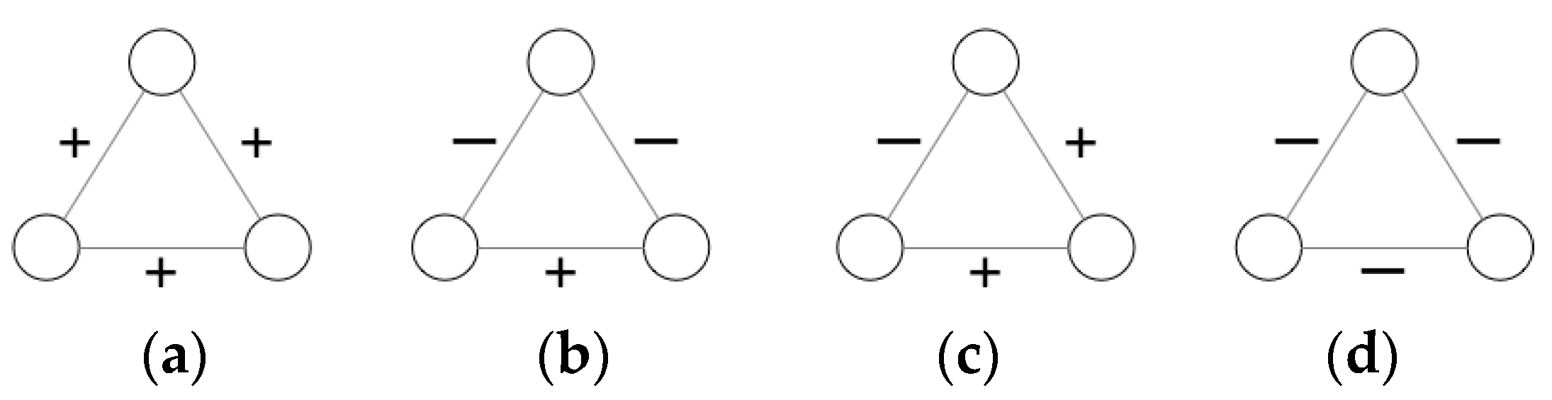
The most common theory associated with signed social networks is the “social balance theory”, which intuitively can be interpreted as “my friend’s friend is my friend”, “my friend’s enemy is my enemy”, “my enemy’s friend is my enemy”, and “my enemy’s enemy is my friend”. Below, we present a definition, in that a graph is balanced if any part of the graph does not conflict with the “social balance theory”.
Figure 1 illustrates the “social balance theory”, where the signed “+” denotes “friend”/“positive”/“trust” and “−” denotes “enemy”/“negative”/“distrust”, subgraphs (a) and (b) are balanced, and (c) and (d) are unbalanced.
References [10,11] show that networks following the concept of balance can cluster into two perfect adversarial groups. In our previous work [12], we also proposed a detection method for maximal balanced cliques in the signed social networks based on the balance theory. A clique is a completely connected subgraph of a graph, which requires all nodes in the subgraph to be connected in pairs with strict constraints. Sometimes, an important node in the dataset has missing pieces of information, which connect it with other nodes, or there is no edge between it and an irrelevant node. As the conditions of clique detection are too strict, this important node is easy to be ignored or is pruned in the process of clique detection [13]. The -Quasi-Cliques have the capacity to solve the mentioned-above problems, as they have more relaxing conditions in comparison to the clique [14].
In this paper, we propose a new model to detect -Quasi-Cliques (it is possible to include the negative edges) for the signed social network, and considering “friendly density” and mutual influence with friends and enemies, we use a method to recompute the weight of edges in the signed social network.
The organizational structure of this paper is: Section 1 introduces the signed social networks and social balanced theory; Section 2 presents related works and analyzes the clustering method for the signed social network in the existing research work; Section 3 explains the basic knowledge about the “friendly density theory” and signed social network and introduces a way to recompute the weight of edges in the signed network and the maximal balanced -Quasi-Clique detect method; Section 4 applies the famous open datasets on our model in the experiment, and determines the optimal threshold for filtering the recomputed weight adjacency matrix and the best value of γ. Finally, Section 5 presents the conclusion of the work and further stages of the research.
2. Related Works
Signed social networks with positive and negative links have attracted considerable attention over the past few years. One of the main challenges in signed network analysis is community detection, which aims to find mutually opposing groups with two characteristics: (1) entities within the same group have as many positive relationships as possible; (2) entities between different groups have as many negative relationships as possible.
The majority of existing algorithms for community detection in signed networks aim to provide hard partitioning of the network, where any node should belong to a single community, such as cliques [15]. However, overlapping communities, in which a node is allowed to belong to multiple communities, are widespread in many real-world networks. Another disadvantage of some existing algorithms is that the final number of clusters k should be the input to the clustering process. However, it may be the case that we do not know k in advance. It will have the limitation of detecting communities by giving clusters the number k.
However, the clustering algorithm of a signed social network cannot succeed to obtain the results only by directly extending the theory and algorithm of the unsigned social network. When edge weights are allowed to be negative, many unsigned social network concepts and algorithms collapse, because they do not work properly in this situation. More recently, studies have been conducted to develop algorithms for efficient methods of clustering signed networks. Doreian and Mrvar [16] proposed a local search strategy similar to Kernighan-Lin algorithm. Yang et al. [17] proposed an agent-based approach, which is essentially a random walk on a graph. Anchuri and Magdon-Ismail1 proposed a hierarchical iterative approach to solve two-way frustrations and signed modularity using spectrum relaxation targets at each level. Bansal et al. [18] also considered the problem of signed graph clustering, although their formula is driven by correlation clustering. They proposed two approximation algorithms and proved the approximation bounds.
Renjie et al. [19] proposed a model, named stable k-core, to measure the stability of a community in signed graphs. Chengyi et al. [20] gave an improved modularity function for signed networks on the basis of the existing modularity function and devised a new community detection algorithm for signed networks. Cadena et al. [21] extended the concept of subgraph density to detect events in signed networks. Ref. [22] is devoted to the study of influence diffusion in signed networks and studies the process of influence diffusion in signed networks. In [23], Tsourakakis et al. considered dense graph detection problems with negative weights. Ordozgoiti et al. [24] proposed a more efficient and scalable approach to this problem.
Qi et al. [25] proposed a framework to solve the problem of negative weights in the signed social networks. In the first step, the authors defined a new computation process to compute the weights between two nodes. They combined the negative edges with the positive ones directly into a parameter called “friendly density”. The proposal of this definition becomes a great contribution to the more objective and reasonable recomputation of edge weights. This paper refers to the definition of friend density to recompute the weights of edges in the next section. Moreover, utilizing the mentioned definition, we consider the six-dimensional space theory [26] to further reasonably compute and obtain a new weight adjacency matrix.
3. Basic Notions and Approach
3.1. Terminologies and Notations
3.1.1. Recalculate the Weights between Friends
A signed social network graph can be noted as G = (V, E, W), where V is a set of nodes, E is a set of weights edges that represents the relationships between the nodes, W is the weight on every edge e, the adjacency matrix A is defined as follows:
For a network G with only positive edges, clustering can be seen as a process that detects all dense subgraphs in G [25]. The computation of dense subgraph C is defined by:
When the G’ is a subgraph of G, w(e) is the weight of edge e in E(G’), |·| is the absolute value of the number. Equation (2) can be generalized to a singed graph where w(e) can be negative. The density of the graph will drop or rise by adding new negative or positive edges.
In a signed network, the relationship between two nodes (i.e., the weights of the edges) may be influenced by rumors/personal bias and may be negative and close to 0, and that negative relationship is subjective and one-sided. When both nodes have positive relationships with their mutual friends, that negative edge is easily influenced by the mutual influence of the friends’ positive relationship. In order to avoid such assertive positive/negative edges caused by considering only the relationship between two nodes, and to better cluster the friendly density clusters, we plan to consider the true state of two nodes based on a more “global” structural environment and adjust their pre-existing or given relationships as necessary. Therefore, we recalculate the relationship weights between two nodes considering the global structural environment and redefine their positive/negative relationship by a reasonable threshold (the selection of the threshold is explored in Section 4 in order not to destroy the original network structure as much as possible).
To solve this problem, reference [25] introduces a weight-completing method, according to which we will obtain the different weights based on length ζ of the path .
Among them, represents the path length, is the maximum value of the path length , the formula traverses all paths of the path length , and for each path , the multiplication of the weights of each edge on the path is calculated. If there are multiple paths of the same length , find the sum of their concatenated products.
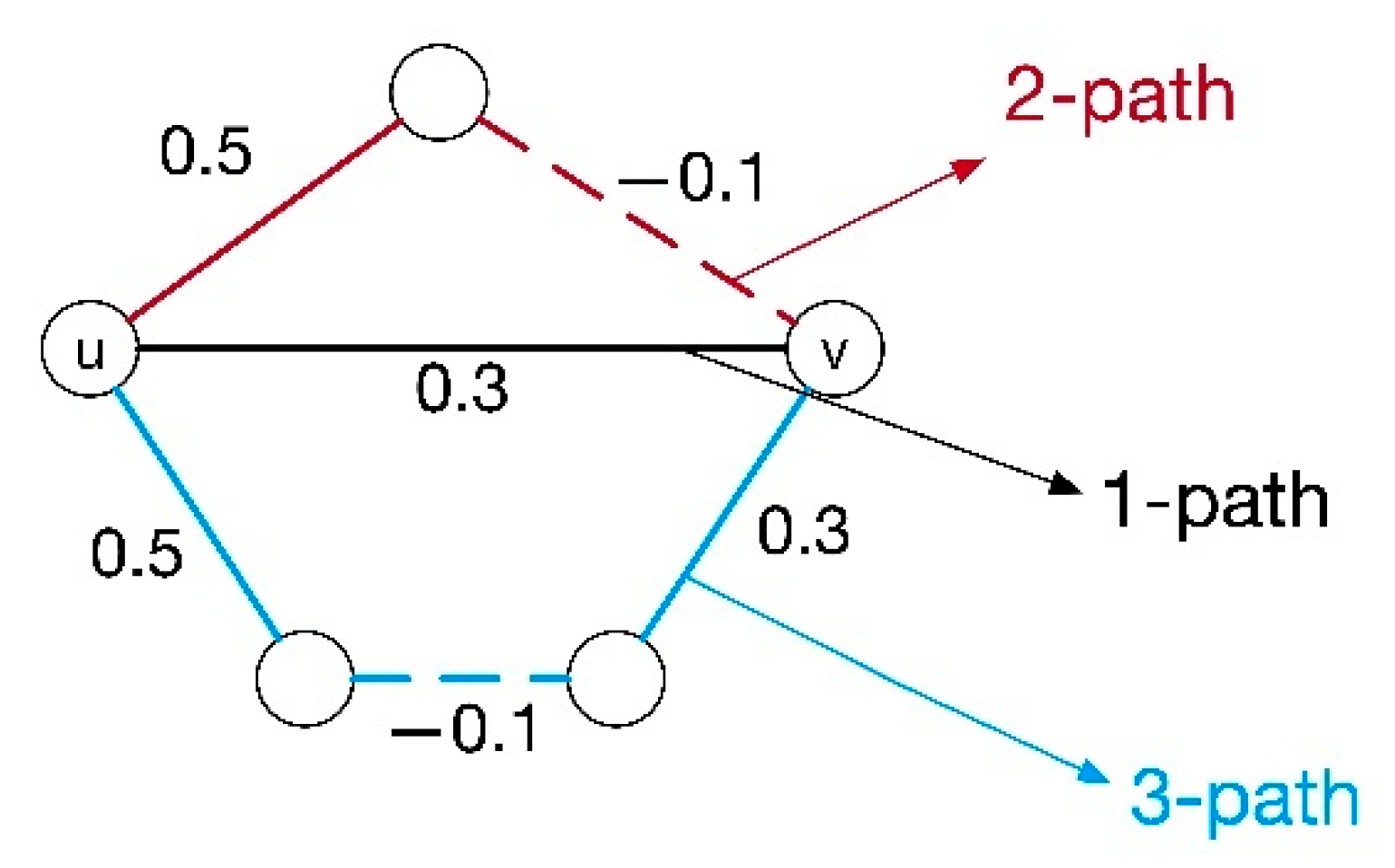
Figure 2 shows an example to explain it. There are three paths between nodes u and v, and the value of each edge represents the positive/negative relationship and weight between the two nodes. When we consider each path equally, = 1, and according to Equation (3), the predicted weight of is
If we use the decaying function , then the predicted weight of is
Comparing the two , when we choose decaying function , the positive relationship between u and v becomes more evident. Similarly, through the calculation of Equation (3), the weight of the negative edge may be more negative.
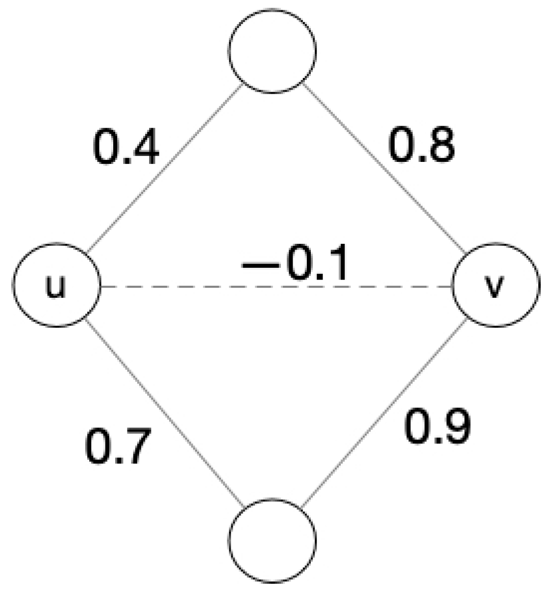
We give an example below to calculate the new relationship value under the mutual influences of common friends even if the direct relationship between nodes u and v is negative, taking into account reasons such as rumors or personal biases: even their direct relationship is negative, and they should gather together in the same cluster. In the example, we choose decaying function. The original graph of this example is shown as Figure 3.
Example:
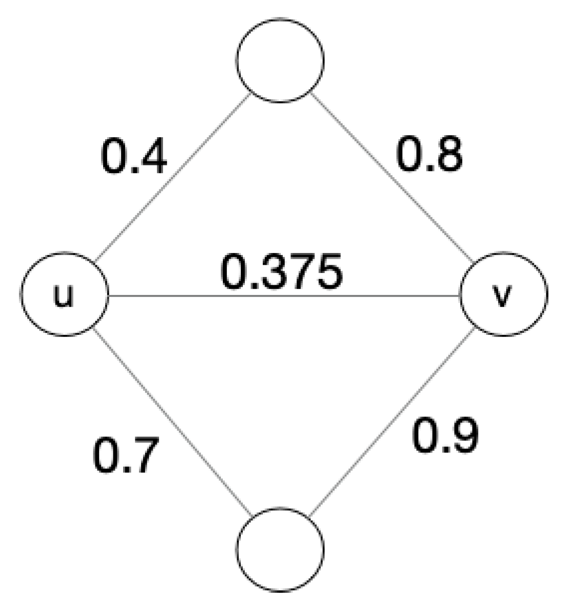
After recalculating the weights between nodes u, v, the network is updated to Figure 4. It is obvious that the network becomes a balanced network, which can be detected in the next step of the balanced community detection algorithm. At this time, the relationship between u and v changes from negative to positive, which is an important reason to use common friends/enemies as parameters for weight calculation. This step can as far as possible avoid the influence of rumors, personal biases, or noisy data collection, and is more comprehensive consider the relationship between two nodes.
However, the process of enumerating all paths for a pair of nodes is NP-hard. To solve the issue, Qi [25] advocates using the (u, v) element in the matrix (), which is equal to the sum of the weights of all paths of length between u and v.
3.1.2. γ-Quasi-Cliques
After completing the graph with the weight of edges in the signed social network, the next step is to detect the -Quasi-Cliques ( is a user-given parameter through which the detection conditions of the Quasi-Cliques can be adjusted. Definition 1 will give a detailed description).
In our previous work [13], we proposed and implemented an enumeration method based on FCA [27,28] for clustering the -Quasi-Cliques. in the social network. This method is suitable for the unsigned graph. Hence, we have to optimize this method to utilize it in the signed social network graph.
Definition 1 (-Quasi-Cliques) [13].
Given a graph G and, if, then the graph G is a Quasi-Cliques and the parameter is(given by users), by-Quasi-Cliques. When V is the set of nodes and, E is the set of edges and. Normally, the range of values foris (0.6, 1].
Definition 2 (Maximal-Quasi-Cliques) [13].
For the graph and node-set
, if G(X) is a -Quasi-Cliques, and there is no more node-set that makes
G(Y) to be a -Quasi-Cliquess, and we call G(X) as Maximal -Quasi-Cliques.
Definition 3 (Formal Concept Analysis, FCA)[21].
Formal Context: Letbe a formal context, where, is the set of objects,is the set of attributes, and I is a binary relation between O and A.
Operators ↑ and↓:Letbe a formal context. The operator↑ and↓ on X⊆ O and Y⊆ A are defined as:
X↑ = {a ∈ A|∀o ∈ X,(o,a) ∈ I}
Y↓ = {o ∈ O|∀a ∈ Y,(o,a) ∈ I}
Formal Concept:For a formal context, ifsatisfies O↑ = A and A↓ = O,is called a Formal Concept, and O is the extent of the concept, A is the intent of the concept. All formal concepts form the formal concept lattice by the partial relation are as (O1, A1) ≤ (O2, A2) ![Land 11 00716 i001]() O1⊆ O2(
O1⊆ O2( ![Land 11 00716 i001]() A1⊇ A2).
A1⊇ A2).
 O1⊆ O2( A1⊇ A2).
In our early work [13], we proved that according to calculating and utilizing the extent or intent of the concept in the formal concept lattice, we can obtain the node number in each -Quasi-Cliques, and then we can calculate the degree in each -Quasi-Cliques and determine whether it satisfies (refer to Definition 1). This process is represented by pseudocode as Algorithm 1:
| Algorithm 1-Quasi-Cliques Detection |
| formal context f 2: begin 3: Formal Concept Lattice ← Construct FCA(f) 4: for each concept ∈ Formal Concept Lattice: 5: value ← * concept.extent.length 6: flag ← True 7: degree ← degree(all nodes of concept) 8: if value > degree: 9: flag = False 10: if flag is True: 11: QuasiCliques.add(concept) 12: return QuasiCliques 13: End |
3.2. Methodology of Maximal Balanced -Quasi-Cliques Detection
3.2.1. Overview
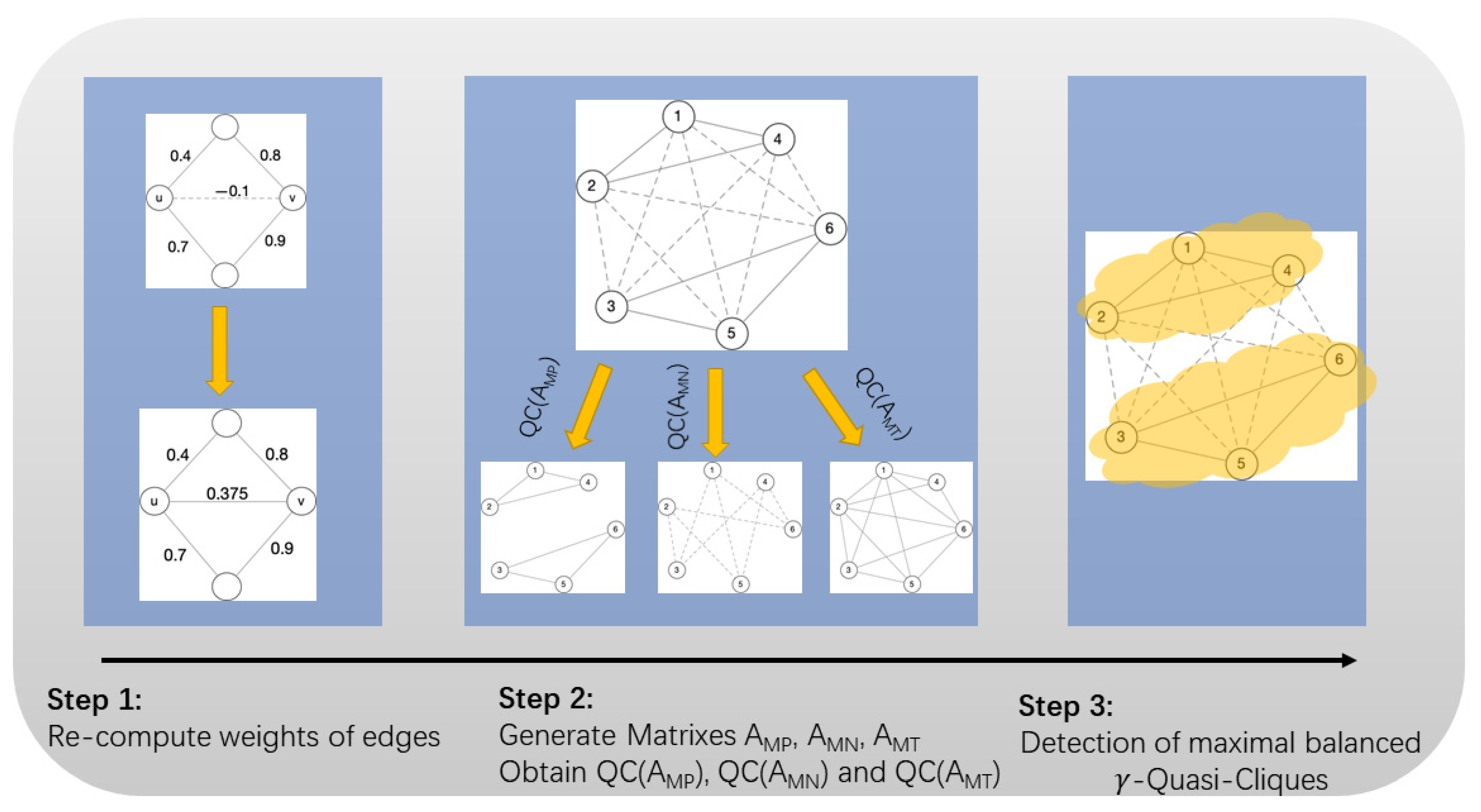
In this subsection, we present the overall framework of the methodology of this paper, shown as Figure 5. The method in this paper is able to be divided into three steps: consider the mutual influence between nodes, re-compute the weights of the edges; generate positive, negative and weightless matrices, and obtain the corresponding Quasi-Cliques, namely QC(AMP), QC(AMN) and QC(AMT); detect maximal balanced -Quasi-Cliques.
3.2.2. Optimization of Weight Matrix Computation
As the value of length in Equation (4) is , a large amount of calculations will still be generated when gradually approaches 0 (); thus, a reasonable maximum length is selected in this paper. As mentioned in Section 2, after referring to the six-dimensional space theory, we only focus on all paths with a path length less than or equal to 6, while choosing the decaying function , we receive the weight of (u, v) equal to:
Since most large social networks are sparse graphs [29], when performing matrix exponentiation on a large social network, we can consider a variety of existing sparse matrix exponentiation methods to improve computational efficiency, e.g., fast exponentiation for matrices [30], which leverage the paradigm to process exponentiation in parallel on GPUs [31]. At the same time, in this paper, we only focus on the first 6th power operation of the matrix instead of the high-power operation. Compared with Equation (4), the complexity of the matrix power operation in this paper is not high.
3.2.3. Our Maximal Balanced -Quasi-Cliques Detection Method
- Step 1 (Complete Weighted Matrix and Prune Data): Make complete weight in the social network graph by Equation (5) and convert it into an adjacency matrix. All elements in the matrix are nonzero after the N power operation of the matrix (N ≤ 6); thus, it is necessary to prune the weight closer to 0 (weight with a more neutral bias). For this, we will provide two thresholds, τ1 and τ2 (given by users).
- If the weight of two nodes is greater than the 1, we regard the edge of these two nodes as a positive edge, noted as 1. If the weight of two nodes is less than 2 (2 is negative), and there is a negative relationship between these two nodes, noted as −1; the remaining nodes are of no relationship and are noted 0. The new adjacency matrix AM is shown in Equation (6).
- Step 2 (rebuild the signed matrixes): Since the -Quasi-Cliques Detection method in Section 3.2.1 is assigned to unweighted and normal social networks (the edges do not have positive/negative relations), in this step, we redefine AM as three matrices. All positive edges are stored in AMP, all negative edges are stored in AMN and edges with weights 1 and −1 are regarded as 1 in AMT, which only indicates whether there is a relationship between the nodes.
- Step 3 (-Quasi-Cliques Detection): Using these three matrixes as input values, perform Quasi-cluster detection to obtain Quasi-Cliques sets QC(AMT), QC(AMP), and QC(AMN), if the Quasi-Cliques in quasi-clusters QC(AMP) and QC(AMN) exist in QC(AMT), then they are our final output: Signed -Quasi-Cliques.
Notes: The QC(AMP) is the set of-Quasi-Cliques with positive edges, the QC(AMN) is the set of-Quasi-Cliques with negative edges, the QC(AMT) is the set of-Quasi-Cliques with positive edges and negative edges (regardless of the sign of the edges). If the-Quasi-Clique E1 and-Quasi-Clique E2 are both in the QC(AMP), there are positive relationships among the nodes in E1 and E2, respectively, the E1 and E2 form a-Quasi-Clique in QC(AMN), and there are negative relationships among the nodes in merger set of E1 and E2. Meanwhile, the merger set of E1 and E2 with positive and negative edges is a-Quasi-Clique in QC(AMT), which means that all nodes in E1 and E2 can form a-Quasi-Clique. At this point, this-Quasi-Clique is a maximal balanced-Quasi-Clique.
To explain the above notes more intuitively, here is an example to illustrate:
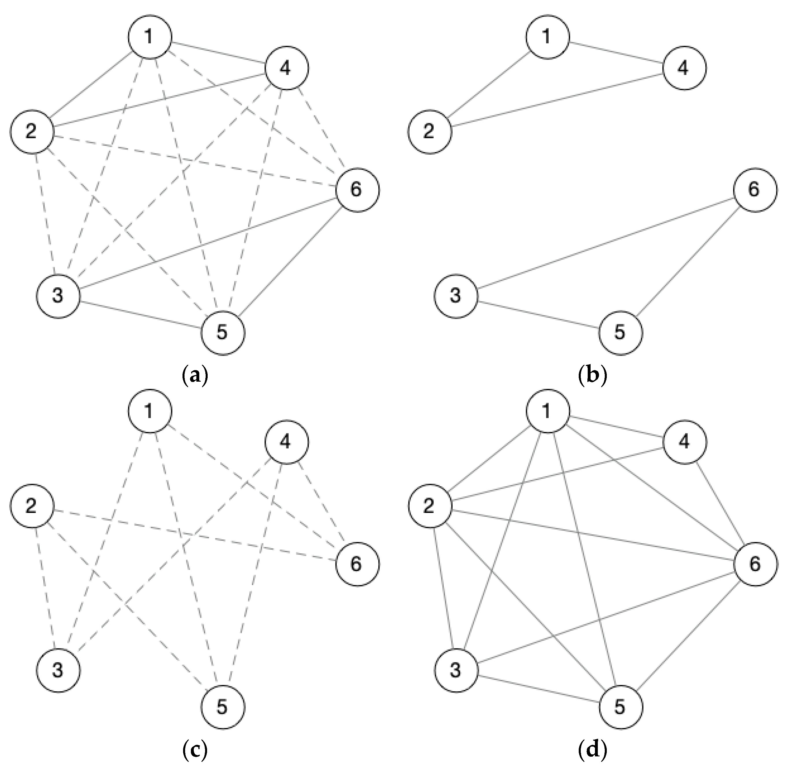
Figure 6a, shows a signed network graph with six nodes, including positive and negative edges between all nodes. According to Equations (7) and (8), the sub-networks corresponding to the positive and negative edges we obtained are shown in Figure 6b and Figure 6c, respectively. Figure 6d conveys all positive and negative edges to unweighted edges. The matrixes corresponding to Figure 6b,c are AMP and AMN, and Figure 6d corresponds to the matrix AMT.
When , in Figure 6b, it is easy to find 2 0.6-Quasi-Cliques with positive edges: {1,2,4} and {3,5,6}. In Figure 6c, {1,2,3,4,5,6} is a 0.6-Quasi-Clique with negative edge., and {1,2,3,4,5,6} is a 0.6-Quasi-Clique without weight in Figure 6d. At this time, we regard {{1,2,4}, {3,5,6}} as a maximal balanced 0.6-Quasi-Clique, in which {1,2,4} and {3,5,6} are two sub-0.6-Quasi-Cliques, which are positive within these two 0.6-Quasi-Cliques, and negative between these two 0.6-Quasi-Cliques.
Algorithm 2 explains steps 1–3.
| Algorithm 2 The overall flow of community detection algorithms |
| graph g, thresholdτ1, τ2 2: begin 3://Complete Weighted Matrix and Prune Data 4: Formal Concept f ← Calculate g by Equation (5) and compare it with threshold τ1, τ2. 5://Rebuild the signed matrixes 6: AMP, AMN, AMT ← Matrix Equation (7) (AM), Matrix Equation (8) (AM), Matrix Equation (9) (AM) 7://Detecting -QuasiCliques 8: -QuasiCliques1, 2, 3 ← Algorithm 1 ( AMP), Algorithm 1 ( AMN), Algorithm 1 ( AMT) 9: for Q1 in QuasiCliques1: 10: for Q2 in QuasiCliques2: 11: if Q1 and Q2 in QuasiCliques3: 12: -Quasi-Cliques ← (Q1, Q2) 13: return Signed -QuasiCliques 14: End |
4. Experiment and Discussion
4.1. Recompute Weight Matrix and Threshold Determination
4.1.1. Dataset and Experimental Environment
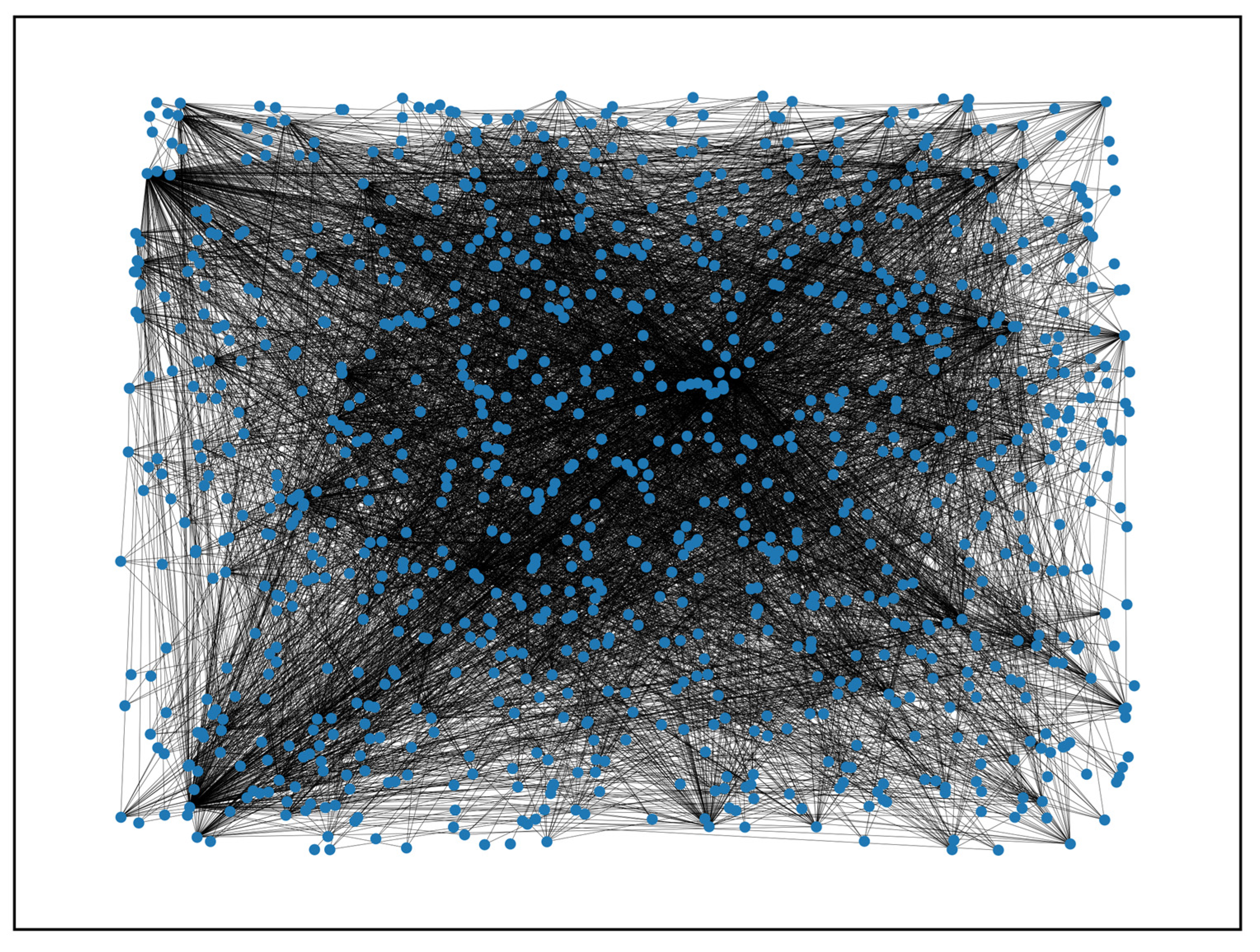
The dataset we use in this section comes from the SNAP public dataset (https://snap.stanford.edu/data/, accessed on 10 July 2009). We apply the “Bitcoin Alpha trust weighted signed network” dataset [32,33] in our experiment. In this dataset, there are 3783 nodes and 24,186 edges, and the weights of edges are on a scale of −10 to +10. The weights are the rating of trust, and members of Bitcoin Alpha rated other members on a scale from −10 (total distrust) to +10 (total trust) in the steps of 1, representing the reputation of users (nodes).
To make the visualization of the clustering results in Section 4.1.2 clearer, we only extracted the first thousand nodes in this dataset to execute our model. Figure 7 is a network graph composed of one thousand nodes.
All experiments in this section run on Windows 10 operating system, Intel Core i7 CPU, 2.90 GHz, and 32 GB RAM.
4.1.2. Threshold Determination
- 1
- The value determination of
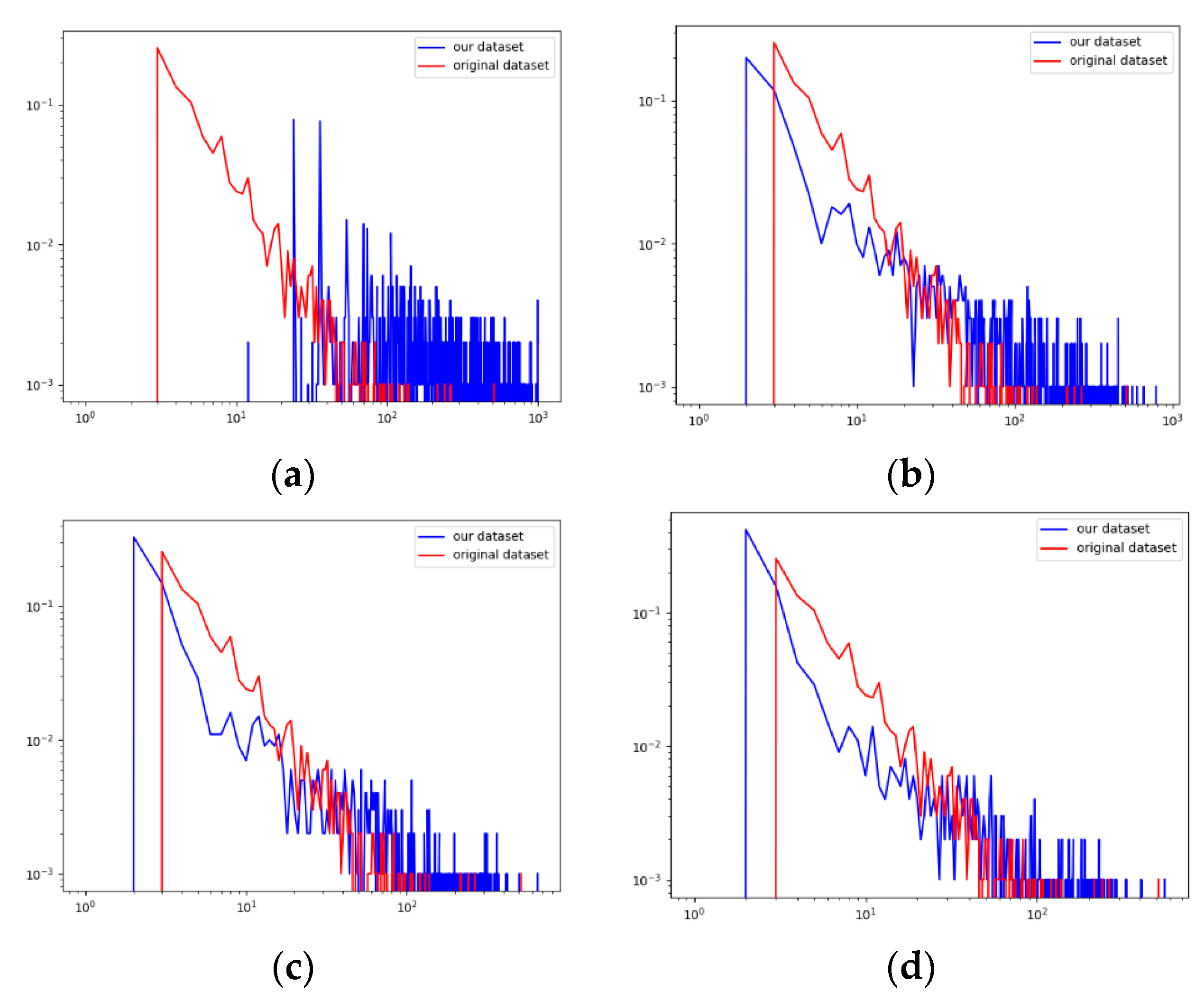
In order to obtain more evident weight edges for positive/negative attitudes of users, we calculated the mean and standard deviation of the matrices AMP and AMN, and pruned the data by giving different threshold ranges of 1 and 2 according to the statistical 68–95–99.7 rule. The four subgraphs in Figure 8 are the distribution of node degrees after setting 1 and 2 in Table 1. It is easily observable that when the values of 1 and 2 are equal to the values in subgraph (d), the pruned data better preserve the structure of the original data.
In addition to comparing the node degree centrality of the four thresholds, we also compare the number of edge prunings under different thresholds.
In order to make the recomputed weight matrix closer to the sparse matrix of the real social network, we prefer to prune edges through a threshold, so as to obtain those edges with more extreme weights. In Table 2, we can see that subgraph (d) has the most pruned edges, excluding redundant data.
- 2
- The value determination of γ
We input the dataset of Figure 8d in the previous subsection as the pruned dataset into our model for the-Quasi-Cliques detection. Table 3 shows the number of Quasi-Cliques and node coverage detected with different values of .
It is known from Table 3 that some nodes overlap in different -Quasi-Cliques, and the higher the degree of overlap of these nodes, the more important they are in the network.
In order to observe the -Quasi-Cliques density with different values more intuitively, we provide a Quasi-Clique node density formula to evaluate the quality of the threshold.
Definition 4.
(Quasi-Clique Node Density, QND)
Table 4shows the results of QND.
From Table 4, we find that when the value of is smaller, the number of detected nodes is larger, the coverage rate in the network is larger, and more maximal balanced -Quasi-clques can be obtained.
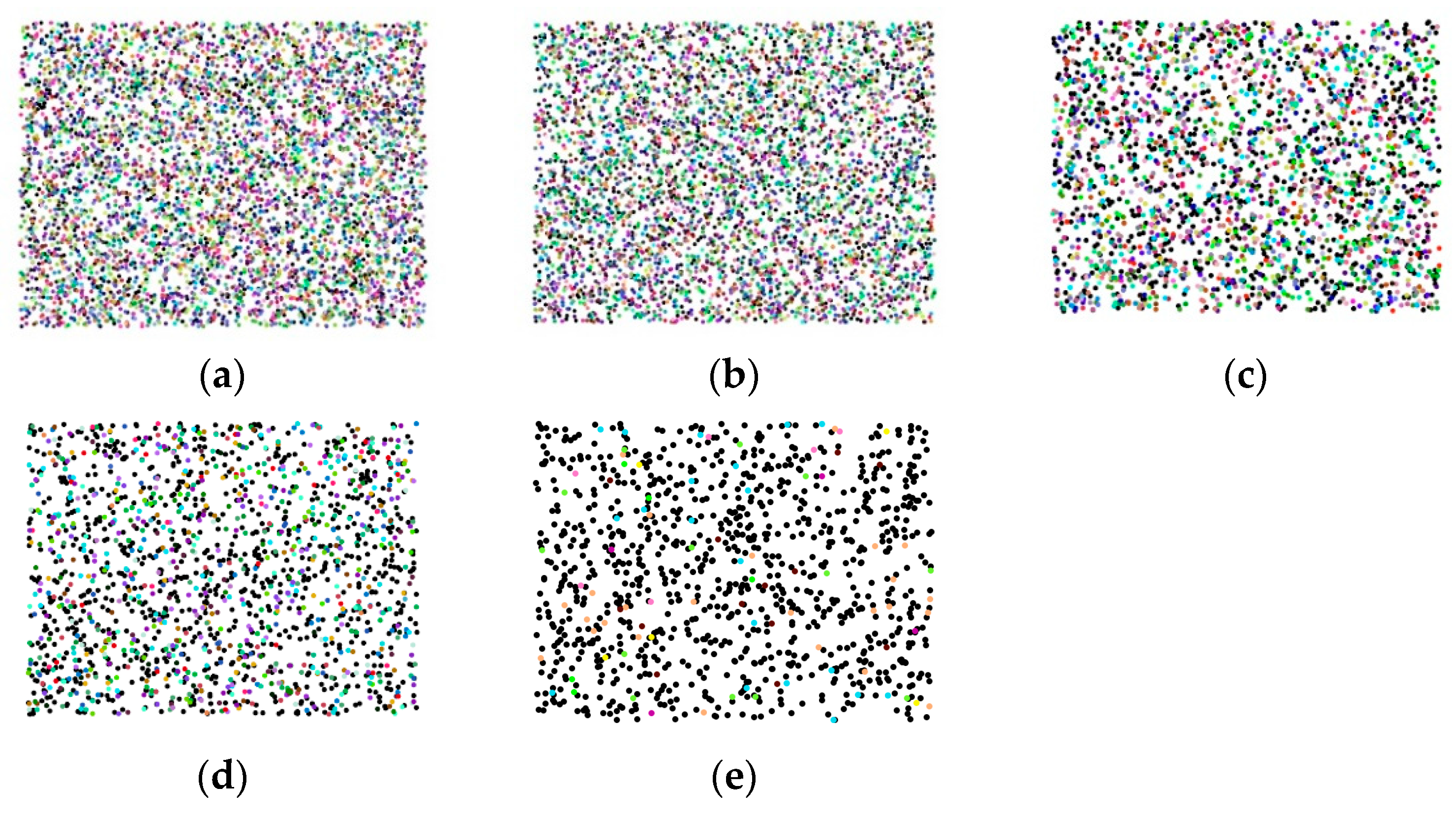
Figure 9a–e represents the nodes distribution of detected -Quasi-Cliques in all cases of = 0.6~1, respectively. In each subgraph, the nodes in the same Quasi-Cliques are represented by the same color. The black nodes are single nodes, which do not belong to any Quasi-Cliques. According to the data in Table 2 and the density of the subgraphs in Figure 5, we can easily find that the density of subgraphs decreases as the value of increases. When , we obtain the densest clustering result.
4.2. Case Study
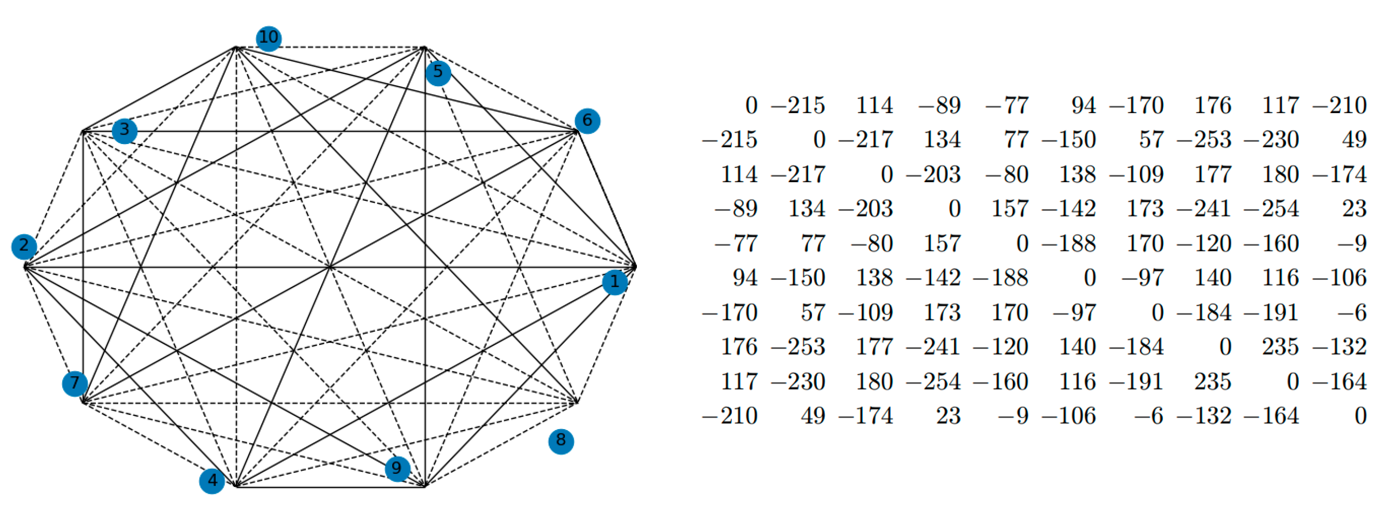
In this subsection, we present a case study to illustrate our method by real-life signed social network data. Figure 10 is a real-world signed network showing a relational network of 10 parties of the Slovene Parliament in 1994 [34]. Here are the signed social network and the matrix.
By completing the weight matrix and running it in our model, we obtain Quasi-Cliques of different sizes according to different values.
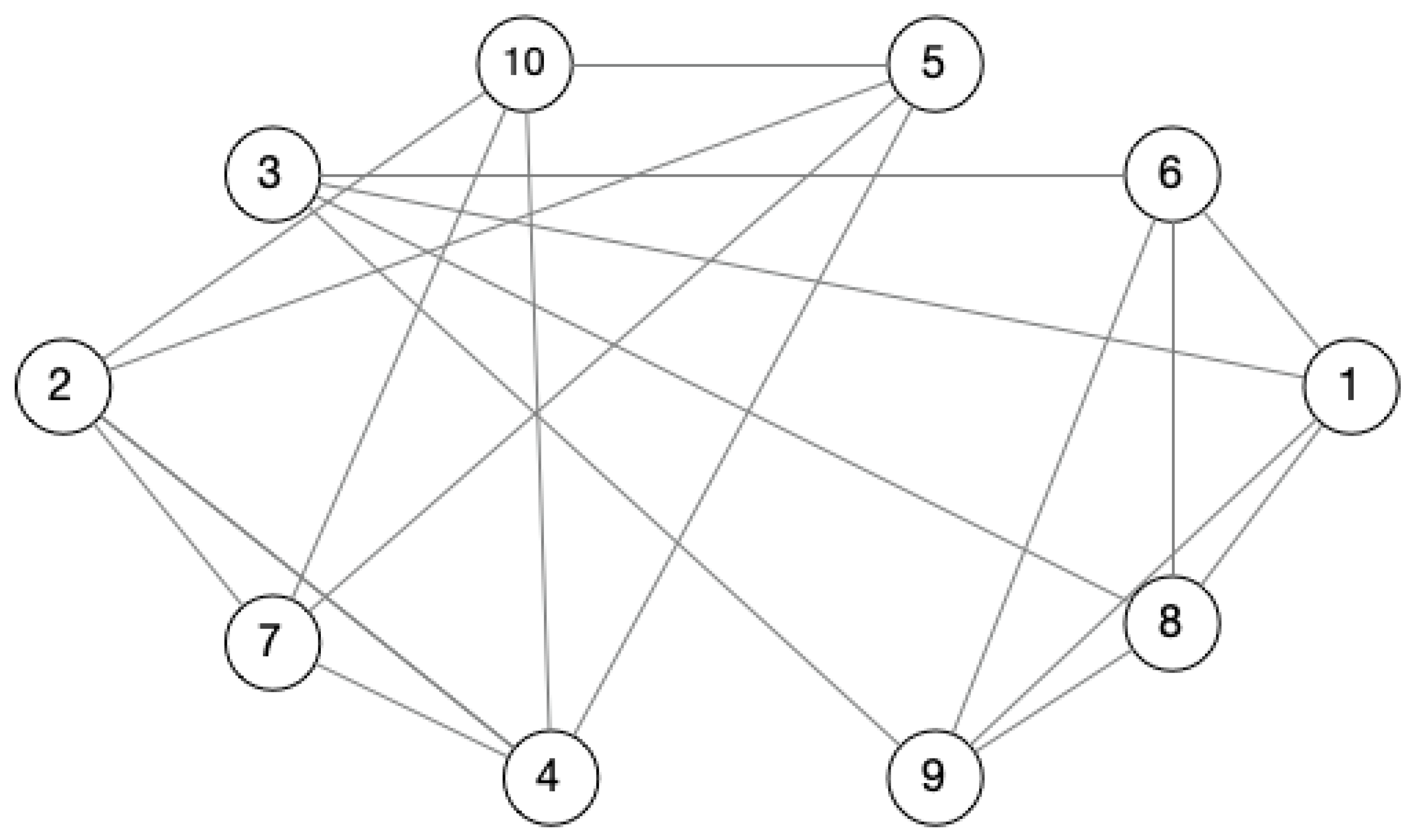
Figure 11 shows the sub-network corresponding to the matrix AMP that retains all positive edges (since a detailed example has been given in the previous section, here, only the positive sub-network is used as an example to illustrate).
When , there are two 0.6-Quasi-Cliques in QC(AMP), which are: {1,3,6,8,9}, {2,4,5,7,10}. For the nodes set {1,3,6,8,9}, γ(|V| − 1) = 0.6 × (5 − 1) = 2.4, and the degree of all nodes is 4; they are larger than 2.4, and they are suitable to the condition degG (V) ≥ γ(|V| − 1).
Similarly, we find one Quasi-Cliques in QC(AMN), which is: {1,3,6,8,9,2,4,5,7,10}. Meanwhile, there is one 0.6-Quasi-Cliques in QC(AMT): {1,3,6,8,9,2,4,5,7,10}. Thus, we can obtain the maximal balanced 0.6-Quasi-Cliques: {{1,3,6,8,9},{2,4,5,7,10}}.
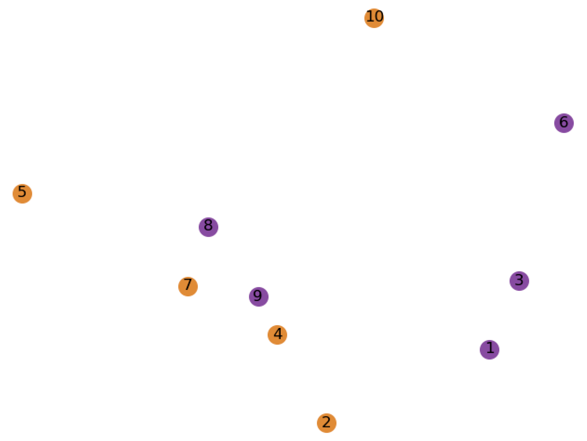
Figure 12 shows the results. The same color of nodes is the same Quasi-Cliques.
Since nodes in a social network correspond to individuals, “places that individuals like to visit” can be regarded as attributes of nodes. Through text mining and other technologies, we are able to mine large social networks with place attributes from social networks such as Twitter, Facebook, and Weibo. Therefore, in real life, different communities have different types of third places to gather, such as cafes, parks, or religious churches. In practical application, we can provide reasonable references for the layout and planning of public places according to the different places mapped to the detected community.
To facilitate understanding the idea of this paper, we simulate that the nodes in the dataset in this case frequently visit some “third places”. Node attributes are as follows in Table 5:
From the above analysis, the social network contains two communities: C1: {1,3,6,8,9} and C2: {2,4,5,7,10}. According to the different attributes of the nodes simulated in Table 5, it is not difficult to find that the nodes in C1 often visit churches, while the nodes in C2 prefer to visit cafes and community centers.
5. Conclusions
Communities in social networks often gather in some urban public places. In order to make reasonable suggestions for urban land division, it is a meaningful topic to study how to effectively detect communities in signed social networks. This paper focuses on mining the maximal balanced -Quasi-Cliques in signed networks for detecting communities. We proposed a model to solve the problems in three steps: First, we recomputed the weights of edges based on the mutual influence of common friends, and we defined and determined some threshold (), (n = 0, 1, 2 and 3) for our pruning data process. Second, we proposed three new definitions of matrixes AMP, AMN and AMT to calculate the -Quasi-Cliques with positive, negative or unweighted edges by FCA method, respectively. Third, We filtered and detected the maximal balanced -Quasi-Cliques. In the experiment, we applied the real-life data to our model, and compared results with different Additionally, to help readers understand the proposed model on an intuitive level, we provided a case study. Experiments proved its effectiveness. In the future, we will consider improving the efficiency of our algorithm for the dynamic signed social network.
Author Contributions
Conceptualization, Y.Y. and D.-S.P.; methodology, Y.Y., and F.H.; validation, Y.Y., S.P., and H.L.; formal analysis, Y.Y.; writing—original draft preparation, Y.Y.; writing—review and editing, D.-S.P.; supervision, D.-S.P. funding acquisition, D.-S.P. All authors have read and agreed to the published version of the manuscript.
Funding
This research was funded by the National Research Foundation of Korea, grant number NRF-2022R1A2C1005921, the BK21 FOUR (Fostering Outstanding Universities for Research), grant number 5199990914048, the Natural Science Basic Research Plan in Shaanxi Province of China (Grant No. 2022JM-371), and the Fundamental Research Funds for the Central Universities (Grant No. GK202103080).
Data Availability Statement
The data presented in this study are openly available in SNAP at https://snap.stanford.edu/data/soc-sign-bitcoin-alpha.html, accessed on 10 July 2009, reference number [32,33,34].
Conflicts of Interest
The authors declare no conflict of interest.
References
- Ramon, O.; Dennis, B. The third place. Qual. Sociol. 1982, 5, 265–284. [Google Scholar]
- Park, J.; State, B.; Bhole, M.; Bailey, M.C.; Ahn, Y.Y. People, Places, and Ties: Landscape of social places and their social network structures. arXiv 2021, arXiv:2101.04737. [Google Scholar]
- HaoYang, L. Research on Key Technologies of Graph Mining; China Knowledge Network: Beijing, China, 2017. [Google Scholar]
- Jung Hee, W.; Ji Woo, P.; Ahn, J.G. Cancer Patient Specific Driver Gene Identification by Personalized Gene Network and PageRank. KIPS Trans. Softw. Data Eng. 2021, 10, 547–554. [Google Scholar]
- Taejin, K.; Heechan, K.; Soowon, L. Automatic Tag Classification from Sound Data for Graph-Based Music Recommendation. KIPS Trans. Softw. Data Eng. 2021, 10, 399–406. [Google Scholar]
- Yongbin, Q.; Cun-quan, Z. A new multimembership clustering method. J. Ind. Manag. Optim. 2007, 3, 619. [Google Scholar]
- Silviu, M.; Bogdan, C.; Talel, A. Building a Signed Network from Interactions in Wikipedia. In Proceedings of the First ACM SIGMOD Workshop on Databases and Social Networks (DBSocial), Athens, Greece, 12 June 2011; pp. 19–24. [Google Scholar]
- Liu, M.M.; Hu, Q.C.; Guo, J.F.; Chen, J. Link prediction algorithm for signed social networks based on local and global tightness. J. Inf. Processing Syst. 2021, 17, 213–226. [Google Scholar]
- Timo, H. Friends and enemies: A model of signed network formation. Theor. Econ. 2017, 12, 1057–1087. [Google Scholar]
- Cartwright, D.; Harary, F. Structural balance: A generalization of Heider’s theory. Psychol. Rev. 1956, 63, 277. [Google Scholar] [CrossRef] [Green Version]
- Harary, F. On local balance and N-balance in signed graphs. Mich. Math. J. 1955, 3, 37–41. [Google Scholar] [CrossRef]
- Yang, Y.; Park, D.S.; Hao, F.; Peng, S.; Hong, M.P.; Lee, H. Detection of Maximal Balanced Clique in Signed Networks Based on Improved Three-Way Concept Lattice and Modified Formal Concept Analysis. 2021. Available online: https://assets.researchsquare.com/files/rs-277245/v1_covered.pdf?c=1631863443 (accessed on 26 April 2021).
- Yang, Y.; Hao, F.; Park, D.S.; Peng, S.; Lee, H.; Mao, M. Modelling Prevention and Control Strategies for COVID-19 Propagation with Patient Contact Networks. Hum.-Cent. Comput. Inf. Sci. 2021, 11, 45. [Google Scholar]
- Guimei, L.; Limsoon, W. Effective Pruning Techniques for Mining Quasi-Cliques. In Proceedings of the Joint European Conference on Machine Learning and Knowledge Discovery in Databases, Antwerp, Belgium, 15–19 September 2008; Springer: Berlin/Heidelberg, Germany, 2008; pp. 33–49. [Google Scholar]
- Fei, H.; Zheng, P.; Laurence, T.Y. Diversified top-k maximal clique detection in Social Internet of Things. Future Gener. Comput. Syst. 2020, 107, 408–417. [Google Scholar]
- Doreian, P.; Mrvar, A. A partitioning approach to structural balance. Soc. Netw. 1996, 18, 149–168. [Google Scholar] [CrossRef]
- Yang, B.; Cheung, W.; Liu, J. Community mining from signed social networks. IEEE Trans. Knowl. Data Eng. 2007, 19, 1333–1348. [Google Scholar] [CrossRef]
- Bansal, N.; Blum, A.; Chawla, S. Correlation clustering. Mach. Learn. 2004, 56, 89–113. [Google Scholar] [CrossRef] [Green Version]
- Sun, R.; Chen, C.; Wang, X.; Zhang, Y.; Wang, X. Stable Community Detection in Signed Social Networks. IEEE Trans. Knowl. Data Eng. 2020. [Google Scholar] [CrossRef]
- Xia, C.; Luo, Y.; Wang, L.; Li, H.-J. A Fast Community Detection Algorithm Based on Reconstructing Signed Networks. IEEE Syst. J. 2022, 16, 614–625. [Google Scholar] [CrossRef]
- Cadena, J.; Vullikanti, A.K.; Aggarwal, C.C. On dense subgraphs in signed network streams. In Proceedings of the 2016 IEEE 16th International Conference on Data Mining (ICDM), Barcelona, Spain, 12–15 December 2016; pp. 51–60. [Google Scholar]
- Li, D.; Liu, J. Modeling influence diffusion over signed social networks. IEEE Trans. Knowl. Data Eng. 2019, 33, 613–625. [Google Scholar] [CrossRef]
- Tsourakakis, C.E.; Chen, T.; Kakimura, N.; Pachocki, J. Novel Dense Subgraph Discovery Primitives: Risk Aversion and Exclusion Queries. In Proceedings of the Joint European Conference on Machine Learning and Knowledge Discovery in Databases, Würzburg, Germany, 6–20 September 2019; Springer: Cham, Switzerland, 2019; pp. 378–394. [Google Scholar]
- Ordozgoiti, B.; Matakos, A.; Gionis, A. Finding large balanced subgraphs in signed networks. In Proceedings of the Web Conference 2020, Taipei, Taiwan, 20–24 April 2020; pp. 1378–1388. [Google Scholar]
- Qi, X.; Luo, R.; Fuller, E.; Luo, R.; Zhang, C.Q. Signed Quasi-Cliques merger: A new clustering method for signed networks with positive and negative edges. Int. J. Pattern Recognit. Artif. Intell. 2016, 30, 1650006. [Google Scholar] [CrossRef]
- Kleinfeld, J. Could it be a big world after all? The six degrees of separation myth. Society 2002, 12, 2–5. [Google Scholar]
- Hao, F.; Min, G.; Pei, Z.; Park, D.S.; Yang, L.T. K-clique community detection in social networks based on formal concept analysis. IEEE Syst. J. 2015, 11, 250–259. [Google Scholar] [CrossRef]
- Yang, Y.; Hao, F.; Pang, B.; Min, G.; Wu, Y. Dynamic maximal cliques detection and evolution management in social internet of things: A formal concept analysis approach. IEEE Trans. Netw. Sci. Eng. 2021. [Google Scholar] [CrossRef]
- Jo, Y.Y.; Kim, S.W.; Bae, D.H. Efficient sparse matrix multiplication on gpu for large social network analysis. In Proceedings of the 24th ACM International on Conference on Information and Knowledge Management, Melbourne, Australia, 18–23 October 2015; pp. 1261–1270. [Google Scholar]
- Okasaki, C. From fast exponentiation to square matrices: An adventure in types. ACM SIGPLAN Not. 1999, 34, 28–35. [Google Scholar] [CrossRef]
- Zhang, J.; Zhou, X. A parallel algorithm for matrix fast exponentiation based on MPI. In Proceedings of the 2018 IEEE 3rd International Conference on Big Data Analysis (ICBDA), Shanghai, China, 9–12 March 2018; pp. 162–165. [Google Scholar]
- Kumar, S.; Spezzano, F.; Subrahmanian, V.S.; Faloutsos, C. Edge Weight Prediction in Weighted Signed Networks. In Proceedings of the 2016 IEEE 16th International Conference on Data Mining (ICDM), Barcelona, Spain, 12–15 December 2016. [Google Scholar]
- Kumar, S.; Hooi, B.; Makhija, D.; Kumar, M.; Subrahmanian, V.S.; Faloutsos, C. REV2: Fraudulent User Prediction in Rating Platforms. In Proceedings of the 11th ACM International Conference on Web Searchand Data Mining (WSDM), Los Angeles, CA, USA, 5–9 February 2018. [Google Scholar]
- Ferligoj, A.; Kramberger, A. An analysis of the slovene parliamentary parties network. Dev. Stat. Methodol. 1996, 12, 209–216. [Google Scholar]
Figure 1.
Balanced and unbalanced triangles. “+” means a positive edge, “−” means a negative edge, where sub-figures (a,b) are balanced triangles and (c,d) are unbalanced triangles.
Figure 1.
Balanced and unbalanced triangles. “+” means a positive edge, “−” means a negative edge, where sub-figures (a,b) are balanced triangles and (c,d) are unbalanced triangles.

Figure 2.
Completing the weight between u and v.

Figure 3.
The original graph g.

Figure 4.
The recomputed weight graph g’.

Figure 5.
The overview of our method.

Figure 6.
A signed network graph and subgraphs of different weighted edges, (a) is the original signed network graph, (b) is the subgraph of (a) with all positive edges, (c) is the subgraph of (a) with all negative edges, and (d) is the unweighted edges graph.
Figure 6.
A signed network graph and subgraphs of different weighted edges, (a) is the original signed network graph, (b) is the subgraph of (a) with all positive edges, (c) is the subgraph of (a) with all negative edges, and (d) is the unweighted edges graph.

Figure 7.
The first thousand nodes are in the Bitcoin Alpha trust weighted signed network.

Figure 8.
The distribution of node degrees with different thresholds. The subgraph (a) is the distribution of node degree with thresholds Mean(AMP) and Mean(AMN); subgraph (b) is the distribution of node degree with thresholds Mean(AMP) + Std(AMP) and Mean(AMN) − Std(AMN); subgraph (c) is the distribution of node degree with thresholds Mean(AMP) + 2 × Std(AMP) and Mean(AMN) − 2 × Std(AMN); subgraph (d) is the distribution of node degree with thresholds Mean(AMP) + 3 × Std(AMP) and Mean(AMN) − 3 × Std(AMN).

Figure 9.
Nodes distribution of the -Quasi-Cliques with different . (a) is the distribution of -Quasi-Cliques when the = 0.6; (b) is the distribution of -Quasi-Cliques when the = 0.7; (c) is the distribution of -Quasi-Cliques when the = 0.8; (d) is the distribution of -Quasi-Cliques when the = 0.9; (e) is the distribution of -Quasi-Cliques when the = 1.

Figure 10.
Ten parties of the Slovene Parliament.

Figure 11.
Subgraph with positive edges.

Figure 12.
Quasi-Cliques of the Slovene Parliament.


Table 1.
Different values of 1 and 2.
| Subgraph (a) | Subgraph (b) | Subgraph (c) | Subgraph (d) | |
|---|---|---|---|---|
| 1 | Mean(AMP) | Mean(AMP) + Std(AMP) | Mean(AMP) + 2 × Std(AMP) | Mean(AMP) + 3 × Std(AMP) |
| 11,377.463 | 66,294.718 | 119,731.322 | 173,936.850 | |
| 2 | Mean(AMN) | Mean(AMN) − Std(AMN) | Mean(AMN) − 2 × Std(AMN) | Mean(AMN) − 3 × Std(AMN) |
| −1074.750 | −18,230.686 | −35,300.547 | −52,414.579 |
Table 2.
The number of edges with different values of 1 and 2.
| Subgraph 8(a) | Subgraph 8(b) | Subgraph 8(c) | Subgraph 8(d) | |
|---|---|---|---|---|
| Number of Prune Edges | 707,589 | 858,691 | 879,438 | 887,651 |
| Number of edges | 292,411 | 141,309 | 120,562 | 112,349 |
Table 3.
The number of Quasi-Cliques and nodes coverage with different values of .
| Number of Quasi-Cliques | 170 | 127 | 67 | 32 | 8 |
| 168 | 146 | 107 | 65 | 43 |
Table 4.
The number of QND with different values of .
| QND | 0.168 | 0.127 | 0.107 | 0.065 | 0.043 |
Table 5.
Simulate attributes of nodes.
| Node | Frequently Visited Third Place |
|---|---|
| 1 | Coffee, Church |
| 2 | Bar, Coffee, Community Center |
| 3 | Church, Park, Coffee |
| 4 | Park, Bar, Coffee, Community Center |
| 5 | Community Center, Coffee |
| 6 | Park, Church |
| 7 | Bar, Community Center, Coffee |
| 8 | Church, Coffee, Bar |
| 9 | Mall, Church |
| 10 | Park, Community Center, Coffee |
Publisher’s Note: MDPI stays neutral with regard to jurisdictional claims in published maps and institutional affiliations. |
© 2022 by the authors. Licensee MDPI, Basel, Switzerland. This article is an open access article distributed under the terms and conditions of the Creative Commons Attribution (CC BY) license (https://creativecommons.org/licenses/by/4.0/).
Share and Cite
MDPI and ACS Style
Yang, Y.; Peng, S.; Park, D.-S.; Hao, F.; Lee, H. A Novel Community Detection Method of Social Networks for the Well-Being of Urban Public Spaces. Land 2022, 11, 716. https://0-doi-org.brum.beds.ac.uk/10.3390/land11050716
AMA Style
Yang Y, Peng S, Park D-S, Hao F, Lee H. A Novel Community Detection Method of Social Networks for the Well-Being of Urban Public Spaces. Land. 2022; 11(5):716. https://0-doi-org.brum.beds.ac.uk/10.3390/land11050716
Chicago/Turabian StyleYang, Yixuan, Sony Peng, Doo-Soon Park, Fei Hao, and Hyejung Lee. 2022. "A Novel Community Detection Method of Social Networks for the Well-Being of Urban Public Spaces" Land 11, no. 5: 716. https://0-doi-org.brum.beds.ac.uk/10.3390/land11050716
Note that from the first issue of 2016, this journal uses article numbers instead of page numbers. See further details here.