3.2. Spatial Variation of LST in Relation to LULC Types
The rapid unplanned expansion of urbanization is a major issue in the urban areas of KMC [
33], which is increasing the artificial area on a large scale, and as a result, the LST is increasing in Kolkata and its surrounding areas [
34]. Therefore, information about the variation and pattern of LST in the different LULC types in every small spatial unit of a city is important on seasonal scales for local-scale adaptation and mitigation [
87]. The highest LST corresponded to artificial land, followed by bare land, vegetation land, grassland, cropland, and bodies of water (
Figure 4). The average LST distribution in the different LULC types followed similar patterns for the different seasons. The average LST of each LULC type decreased continuously from summer to transition, then to winter (
Figure 4), which may be due to the decrease in solar radiation from summer to transition to winter because of the tilted axis of rotation of the Earth. The average LST was 30.432 °C in summer, followed by27.415 °C in transition, and 24.894 °C during the winter season. Artificial land corresponded to the highest LST in all seasons because built-up lands have different thermal bulk properties (heat capacity and thermal conductivity) and radiative properties (albedo and emissivity) [
88]. For this reason, the urban artificial surface absorbs significantly more solar radiation, which causes a change in the energy budget of the urban area, often leading to a higher LST [
89]. Dense buildings also reduce wind speed and block the longwave emissions from the ground, which helps to gather heat inside the city and increase the temperature [
90]. The second-highest LST was observed in bare lands. This result is quite similar to the study in [
90], wherein they revealed that bare soil’s heat capacity is minimal with a lower moisture content and evapotranspiration rate, resulting in the rapid rate of heating during the daytime. Therefore, high temperature surfaces were developed in exposed areas. The lowest temperatures were observed in bodies of water, followed by croplands, grasslands, and vegetation lands. Plants and bodies of water act as an evaporation cooling system by spreading the moisture to the atmosphere through evaporation, resulting in a reduction of the LST [
90]. Furthermore, due to the higher heat capacity of bodies of water than land surface, water surface temperatures increase slowly, so low temperatures are observed in bodies of water compared to land surfaces under the same solar radiation [
90]. Vegetation also creates an albedo effect that is 15% higher than urban surfaces due to the small absorption of heat and higher reflectance [
91]. Furthermore, the canopy of vegetation increases the shade effect, which reduces incident radiation [
89]. The average temperature of croplands was lower than that of grasslands and vegetation lands, which may be due to the croplands acting as vegetation and irrigation lands, and irrigation decreases land surface temperatures during daytime [
92]. Therefore, green surfaces and bodies of water are the major factors that mitigate the increase in LST. This result is quite similar to the study from [
93], which revealed that high temperatures and low temperatures correspond to built-up areas and bodies of water in three megacities in China.
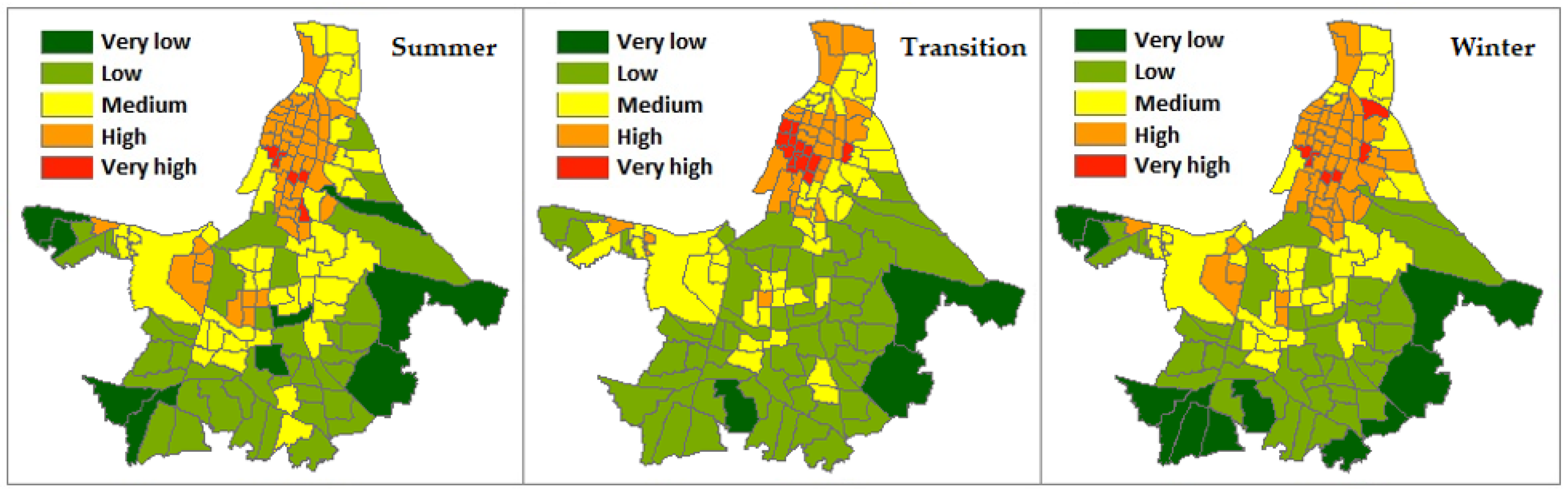
Therefore, it is clear from
Figure 5 and
Figure 6 that the high-temperature ward as well as the regions were mostly distributed in the middle-northern parts and somewhere in the western parts of highly urbanized areas, where artificial land cover predominated, lacked bodies of water and green cover (
Figure 3). There is a large number of previous studies [
77,
93] that also revealed that artificial land surfaces are highly related to a high LST. The number of very high temperature wards was 5, 12, and 6 in the summer, transition, and winter seasons, respectively (
Figure 6). The number of very low temperature wards was 9, 3, and 11 in the summer, transition, and winter seasons, respectively (
Figure 6). Low and very low temperature wards were distributed in the surrounding areas that dominate the eastern part of the study area, which is most likely due to the distribution of green zones and bodies of water (
Figure 3).
3.3. Effects of Each Category of Influencing Factors in the Different Season
The OLS regression analysis showed that many influencing factors were significantly fitted across the cities for the different seasons (
Table 6). The relationship between the LST and influencing factors during the different seasons are shown in
Figure S2. The significantly fitted or correlated variables are those that are statistically significant at the 5% significance level and are later chosen for all-subsets regression modelling.
The surface properties characterize the highest explanatory rate compared to the other categories of variables for all seasons (
Table 7). Various studies also used surface biophysical properties to explain the variability of LST [
24,
26], and reported that the surface cover properties are the most influencing factors of urban LST [
72] because the surface biophysical indices contain more information about particular properties [
24]. Our results are also consistent with these studies. The explanatory rates (R-squared) of the surface properties were 78.9%, 78.6%, and 70.5% in the summer, winter, and transition seasons, respectively. This indicates, along with increasing rainfall, that the explanatory rate of surface properties has decreased, resulting in surface properties being more important for explaining the LST in the winter and summer season when the temperature is relatively low and high with low rainfall. This result agreed quite well with the study from [
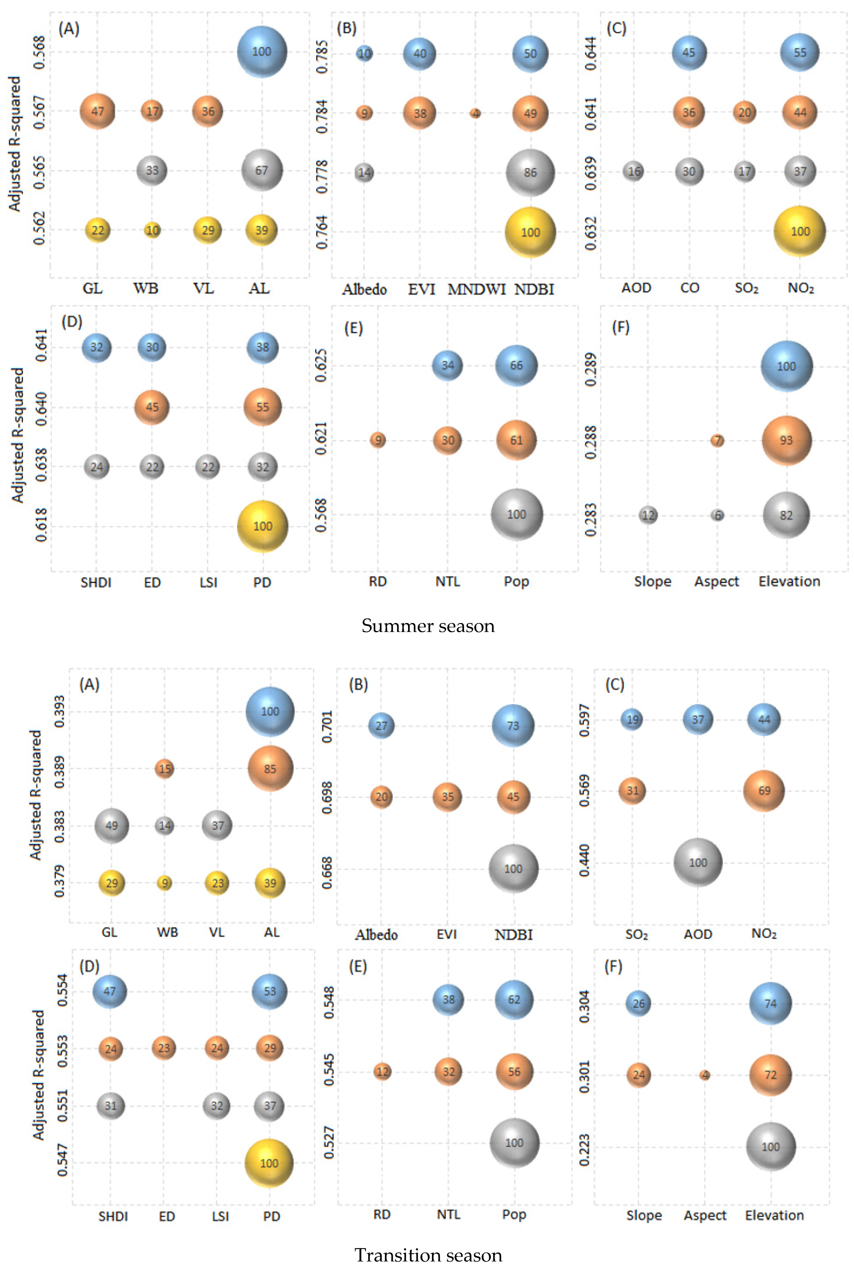
24], which reported that biophysical parameters could explain more of the variation in LST during low- or high-temperature seasons. In the summer season, the combination of
NDBI,
EVI, and albedo gave the highest explanatory rate (
Figure 7A), and
NDBI was the most significant contributing factor (50%), followed by
EVI (40%) and albedo (10%). In the transition season, the combination of
NDBI and albedo gave the highest explanatory rates with an independent effect of 73% and 27%, respectively (
Figure 7B). In the winter season, the highest explanatory rate was received from the combination of all surface properties, and
NDBI was the most significant contributing factor (41%) compared to
EVI (39%), albedo (15%), and
MNDWI (5%) (
Figure 7C). Compared to the summer and transition seasons, the number of factors was increased to explain the variation in LST during the winter season, which indicates that during low temperatures, more factors were required to explain the variation in LST. Conversely, in the transition season, only a few variables of surface properties (
NDBI and albedo) are entered into the optimal model to explain the variation in LST with an explanatory rate of 70.5%, which indicates that there are other robust factors that control the variability of LST.
NDBI and albedo were constantly selected for the optimal model for all the seasons, which indicates that the combination of
NDBI and albedo is important to explain the more variation of LST for all seasons.
EVI was selected for the summer and winter seasons, and
MNDWI was selected for the winter—in combination with other variables—which indicates that
EVI and
MNDWI have seasonal importance for explaining the LST in combination with other surface properties. Furthermore, the OLS regression explanatory rates of
EVI and
NDBI were higher with a high significance (
Table 6), which is consistent with previous studies. Various studies also reported that
MNDWI or bodies of water have a highly significant effect on LST [
26,
90], but in this study,
MNDWI had a very low explanatory rate, which was mainly due to the total area of bodies of water being small (3.41%) and concentrated in one particular site (eastern parts) of the study area (
Table 5 and
Figure 3).
In the categories of pollutant parameters, different factors were entered for the optimal models for the different seasons. Previous studies have always ignored the category of pollutant parameters, but pollutant parameters could explain the 64.9% variation in the LST during the summer, 60.6% variation during the transition, and 51.1% variation during the winter season (
Table 7). This indicates that the explanatory rate of pollutant parameters has decreased with the decrease in LST, thereby resulting pollutant parameters could explain more variation of LST when the temperature is relatively high in the study area. In the summer season, only CO and NO
2 were entered into the optimal model with an independent effect of 55% and 45%, respectively (
Figure 7A). In the transition season, the combination of NO
2, AOD, and SO
2 gave the highest explanatory rate, and NO
2 had the largest independent effect (44%), followed by AOD (37%) and SO
2 (19%) (
Figure 7B). In the winter season, AOD and SO
2 gave the highest explanatory rate, with an independent effect of 65% and 35%, respectively (
Figure 7C). Therefore, more factors were required to explain the variation in LST during the rainy season, and limited factors were required during the relatively low or high temperatures of low rainfall seasons. That is to say, AOD and SO
2 could explain the high levels of variation in LST when the temperature was relatively low in the study area. AOD and SO
2 were also the highest explanatory factors during the winter season in OLS regression (
Table 6). However, when the summer season temperatures are high, the combination of NO
2 and CO could explain the high levels of variation in LST. Furthermore, in the OLS regression, NO
2 was the highest explanatory factor, followed by CO, SO
2, and AOD (
Table 6) during the summer season.
Regarding socio-economic factors, the explanatory rates were greater in winter (68.2%), followed by the summer (64.9%) and transition season (60.6%) (
Table 7). The combination of population and NTL gave the largest explanatory rates for all seasons with independent effects of 66% and 34% in the summer (
Figure 7A), 62% and 38% in the transition (
Figure 7B), and 68% and 32% in the winter (
Figure 7C), respectively. Furthermore, in OLS regression, population and NTL were strongly correlated with LST for all seasons (
Table 6), which is consistent with previous studies [
23]. The explanatory rate of road density was 20.99%, 20.25%, and 22.14% during the summer, transition, and winter seasons, respectively (
Table 6). The higher explanatory rate in winter indicates that when LST is relatively low (winter season), the effect of socio-economic parameters on LST variation is high. Various prior studies also reported that the amount of anthropogenic heat released over cities due to socio-economic activities is greater in winter than in summer [
94,
95], which indicated that regulating the population size could mitigate the LST [
96]. Basically, nighttime lights are always associated with a high per capita income [
97], which indicates high economic activity [
98].
The explanatory rate of LST variation by topographic factors was relatively low compared to other groups of variables (
Table 7). Only the elevation factor entered the optimal model for the summer season, which was also the higher interpreter compared to other topographic factors in the OLS regression (
Figure 7A). For the transition and winter seasons, combinations of elevation and slope gave the highest explanatory rate with an independent effect of 74% and 26% in the transition, and 68% and 32% in the winter, respectively (
Figure 7B,C); the explanatory rate was higher in transition (31.4%) than in summer (29.4%) and winter (25.1%). However, all the significant topographic factors were positively related with LST (
Table 6), which is opposite to the study by Peng et al. (2020) that reported that topographic parameters, such as slope and elevation, generally have a negative effect on LST because as elevation increases, the air becomes thinner and loses its capability to retain heat. However, our study depicts opposite results, and this was mainly because of two reasons: firstly, a very small variation in topography (2.42 to 17.48 m) throughout the study regions, so there may be no significant difference in air density in the study region; secondly, the low elevation and low slope areas were covered by green covers and bodies of water, and the high elevation and high slope areas were covered by human activities as well as artificial lands. Therefore, artificial lands with a high elevation and sloping regions had a negligible infiltration rate and helped to quickly dry up quickly downward water flows due to the force of gravity. Given this, the lower availability of moisture helped to quickly heat up elevated and sloping regions, and the high availability of moisture helped to reduce the temperature in low land areas. This might also cause the topographic parameters that are largely explained by the variability in LST during the transition season compared to the summer and winter seasons.
Landscape configurations have higher explanatory power compared to landscape compositions, which explain the variation in LST for all seasons (
Table 7). Several previous studies [
25,
99] have reported that landscape configurations could explain more of the variation in LST than landscape composition. Again, [
24,
26] reported that the impact of landscape configurations is limited compared to landscape compositions. Therefore, it is not possible to make any reasonable comparisons with other studies in different cities as different regions and study periods may differentiate the effect of landscape configurations on LST. Except for MSI, all other configuration factors had a strong negative correlation with LST in OLS regression (
Table 6). The explanatory rates of the optimum model were 64.5%, 56.1%, and 54.3% for the summer, transition, and winter, respectively. This also indicates, along with the decrease in LST, that the explanatory rate of the landscape configurations decreased, and as a result, the landscape configurations could better explain the higher level of variation in LST when the temperature was high in the study area. During the summer season, the combination of PD, ED, and SHDI gave the highest explanatory rate (
Figure 7A), and the PD was the largest contributor (38%), followed by SHDI (32%) and ED (30%). During the transition season, we found that the highest explanatory rate was from the combination of PD and SHDI, which have an independent effect of 53% and 47%, respectively (
Figure 7B). During the winter season, the combination of all significant landscape configurations, such as PD, ED, SHDI, and LSI, gave the highest explanatory rates, with independent effects of 33%, 21%, 24%, and 22%, respectively (
Figure 7C). It is also noted that in the winter season, the highest number of factors were required of landscape configurations for the optimal model with the lowest explanatory rate compared to other seasons to explain the variation in LST, thereby indicating that the variation in LST became more complicated during the winter season. PD and SHDI were entered into the optimal model for all seasons, given that the combination of PD and SHDI was important for explaining the high levels of variation in LST for all seasons. However, ED was entered into the optimal model for the summer and winter seasons, and LSI was only entered for the winter, which indicates that ED and LSI have seasonal importance that explains the higher levels of variation in LST in combination with the other landscape configurations.
The explanatory rates for landscape compositions were 57.1%, 39.8%, and 49.5% during the summer, transition, and winter, respectively (
Table 7). In the summer and transition season, only artificial land (AL) entered into the optimal model (
Figure 7A,B), but in winter, the combination of vegetation land (VL), grassland (GL) and bodies of water (WB) gave the highest explanatory rates with an independent effect of 29%, 61%, and 10%, respectively (
Figure 7C). This result indicates that the variation in LST was more likely affected by one dominant landscape composition factor (artificial land) when the temperature was relatively high, but when the temperature was low, the proportion of green space cover and bodies of water could explain more of the variation in LST, thereby resulting in the higher number of variables were required to explain the variation in LST during the winter season. The artificial land in OLS regression also gave the highest explanation in summer than in other seasons (
Table 6). This finding is consistent with previous studies, which suggest that the higher the proportion of artificial land, the stronger the effect on LST during the summer [
24] due to the intense heating of urban artificial surfaces [
100,
101]. During the winter season, there is a lack of adequate solar radiation, so the combination of green cover areas and bodies of water play a greater role compared to the single-level artificial surface that has been used to explain the variation in LST. Although bodies of water and bare lands were associated with a lower LST and higher LST, respectively (
Figure 4), the explanatory rates of bodies of water were only 19.09%, 11.75%, and 11.91% during the summer, transition, and winter, respectively. Moreover, the explanatory rate of bare land was not significant for any of the seasons. This may be due to the low availability of bodies of water and bare lands in the study area (
Figure 3 and
Table 5).
However, in the summer and transition season, surface properties gave highest explanatory rates, followed by pollutant parameters, landscape configurations, socio-economic parameters, and topographic parameters. In contrast, in the winter season, surface properties gave the highest explanatory rates, followed by socio-economic parameters, pollutant parameters, landscape configurations, and topographic parameters. In addition, the explanatory rate (R-squared value) of all factors in the OLS regression varied for the different seasons. Therefore, the effects of influencing factors on LST are seasonally changed.
3.4. Integrated Effects of Al l Influencing Factors in the Different Seasons
In heterogeneous urban environments, LST is not controlled by a single factor or by single categories of factors [
102]. Previous studies [
24,
26] used a large number of influencing factors to explain the variability in LST, but in this study, we have additionally used two more categories of influencing factors, pollutant parameters and topographic parameters. A total of 25 influencing factors from 6 categories of variables were used in this study, and 22, 20, and 21 influencing factors were included for all-subsets regression for the summer, transition, and winter season, respectively.
Ten significant factors, NO
2, albedo,
EVI,
MNDWI,
NDBI, slope, LSI, NTL, population, and VL, were entered into the optimal model for the summer season (
Figure 8A), for which the explanatory rate was 89.4% (
Table 8). For the transition season, 11 explanatory variables were included, SO
2,
NDBI, slope, elevation, PD, ED, LSI, NTL, population, AL, and GL (
Figure 8B), for which the explanatory rate was 81.4% (
Table 8). For the winter season, the explanatory rate was 88.7% (
Table 8) and 12 variables were included: AOD, SO
2,
EVI,
MNDWI,
NDBI, elevation, LSI, SHDI, NTL, population, AL, and WB (
Figure 8C). Therefore, from summer to transition to winter, the number of factors for the optimal model was increased, indicating that with a decrease in the LST, more factors were required to explain the variation in LST. This result is consistent with the study from [
24], which revealed that more factors are required to explain the variability of LST from the warm to the cold season. For the transition season, the explanatory rate was far lower (81.4%) than the summer (89.4%) and winter (88.7%), which indicates that there are other important factors controlling the variation in LST during rainy periods. As more than 9 influencing factors were entered into the optimal models for all seasons, we ran the HP model 100 times with different orders of the set of variables, as recommended by [
86], then the average of the 100 runs was taken to identify the independent effects. The independent effects of the optimum models for each season are shown in
Figure 9.
NDBI was the dominant contributing factor (19.49%), followed by
EVI (16.23%), NO
2 (15.22%), population (13.15%), LSI (11.79%), VL (9.78%), NTL (8.12%), albedo (3.69%), slope (1.59%), and
MNDWI (0.93%) for the summer. Therefore, in the summer season, the sum of surface properties independently contributed 39.41% (
NDBI,
EVI, and albedo), followed by socio-economic parameters (21.27%), pollutant parameters (15.22%), landscape configuration (11.79%) and compositions (10.71%), and topographic parameters (1.59%). For the transition season,
NDBI also was the dominant factor (15.95%) for LST variations, while PD, population, LSI, ED, NTL, AL, GL, elevation, SO
2, and slope contributed 11.16%, 10.81%, 10.53%, 10.31%, 8.58%, 8.27%, 7.33%, 6.29%, 5.87% and 4.93%, respectively. For the transition season, the sum of landscape configuration made the largest contribution (32%), followed by socio-economic parameters (19.39%), surface properties (15.95%), landscape compositions (15.6%), topographic parameters (11.22%), and pollutant parameters (5.87%). For the winter season,
EVI and
NDBI were the dominant contributors (14.78% and 14.66%, respectively), whereas the independent effects of the other selected factors were 12.31%, 9.26%, 9.13%, 8.47%, 8.37%, 6.42%, 4.74%, 4.37%, 4.27%, and 3.22% for population, AL, NTL, LSI, SHDI, AOD, elevation, SO
2, WB, and
MNDWI, respectively. In the winter season, the sum of surface properties contributed 33.66%, followed by socio-economic parameters (21.44%), landscape configurations (16.84%) and compositions (13.63%), pollutant parameters (10.79%), and topographic parameters (4.74%). Therefore, surface properties largely contributed during the summer season, compared to the winter season when the temperature was relatively high and low with less rainfall. However, landscape configurations largely contributed during the transition season when the temperature was medium with high rainfall. The socio-economic properties (19.39–21.44%) and landscape compositions (10.71–15.6%) had slightly consistent contributions for all the seasons. The pollutant parameters and topographic parameters also largely contributed to LST during the summer (15.22%) and transition seasons (11.22%), respectively. Therefore, there were significant differences for the contributions from the influencing factors for different seasons. This result is similar to the study from [
24,
103] and revealed that various influencing factors behave differently for the different seasons. The first five factors contributed 75.89%, 58.76%, and 60.14% for the summer, transition and winter seasons, respectively. This result also indicated the high temperature (summer season) variation in LST was more likely affected by the combination of a few dominant factors, and during the transition and winter season, the independent effect tended to spread among the variables.


 ,
, 


