
Monitoring of Water and Tillage Soil Erosion in Agricultural Basins, a Comparison of Measurements Acquired by Differential Interferometric Analysis of Sentinel TopSAR Images and a Terrestrial LIDAR System
 , , , , and
Abstract
:1. Introduction
- The accuracy of the measurements
- Coherence loss boundary
- The effect of soil moisture
- The effect of soil decompaction
- Type of vegetation
2. Materials and Methods
2.1. Study Area
- Accessible and monitorable: These enabled checks to be made during satellite overflights for the presence of walkers, livestock, or machines that might figure as variations in the ground surface.
- Clear: The scant and small vegetation in the plot would not affect the differential interferometry analysis of the SAR images [44]. However, it would affect the measurements made by the LIDAR system.
- Size: Large enough to contain several interferometry result raster cells (13.93 m side), but not so much to make the daily terrestrial LIDAR work unaffordable.
- An area with surrounding plots suitable for comparison: Plots used in this kind of study need to have a high coherence contrast with bordering plots [44,45]. This allows their localization in coherence maps produced by differential interferometry. Since the present study required a plot with almost naked, erodible ground (low coherence), it was desirable that it be surrounded by plots with high coherence (e.g., asphalted or built-up areas).
- A nearby control plot was available: A nearby high-coherence control plot is desirable since it can provide the reference for zero deformation [37].
2.2. The Sentinel-1 Mission
2.3. Data Acquisition
2.3.1. TopSAR Images for Differential Interferometric Analysis
2.3.2. In Situ Surface Measurement Using the Terrestrial LIDAR System
2.4. Analytical Methods. Differential Interferometry
- flat = the curvature of the Earth.
- elevation = topography.
- displacement = deformations of the terrain between the two acquisitions of information.
- atmosphere = differences in relative humidity, pressure, and temperature between information acquisitions.
- noise = changes over time in volume scattering and acquisition angles, etc.
- = Temporal factor. This cannot be avoided and is due to the differences in the ground occurring between the two information acquisitions; it is important to the present work.
- = Geometric factor. This is caused by errors in the orbit of the satellites; it can be partially accounted for.
- = Volumetric factor. Unavoidable due to the presence of vegetation.
- = Processing factor. Caused by errors of calculation; this should be avoided.
2.4.1. Software
2.4.2. Coregistering and Interferogram Construction
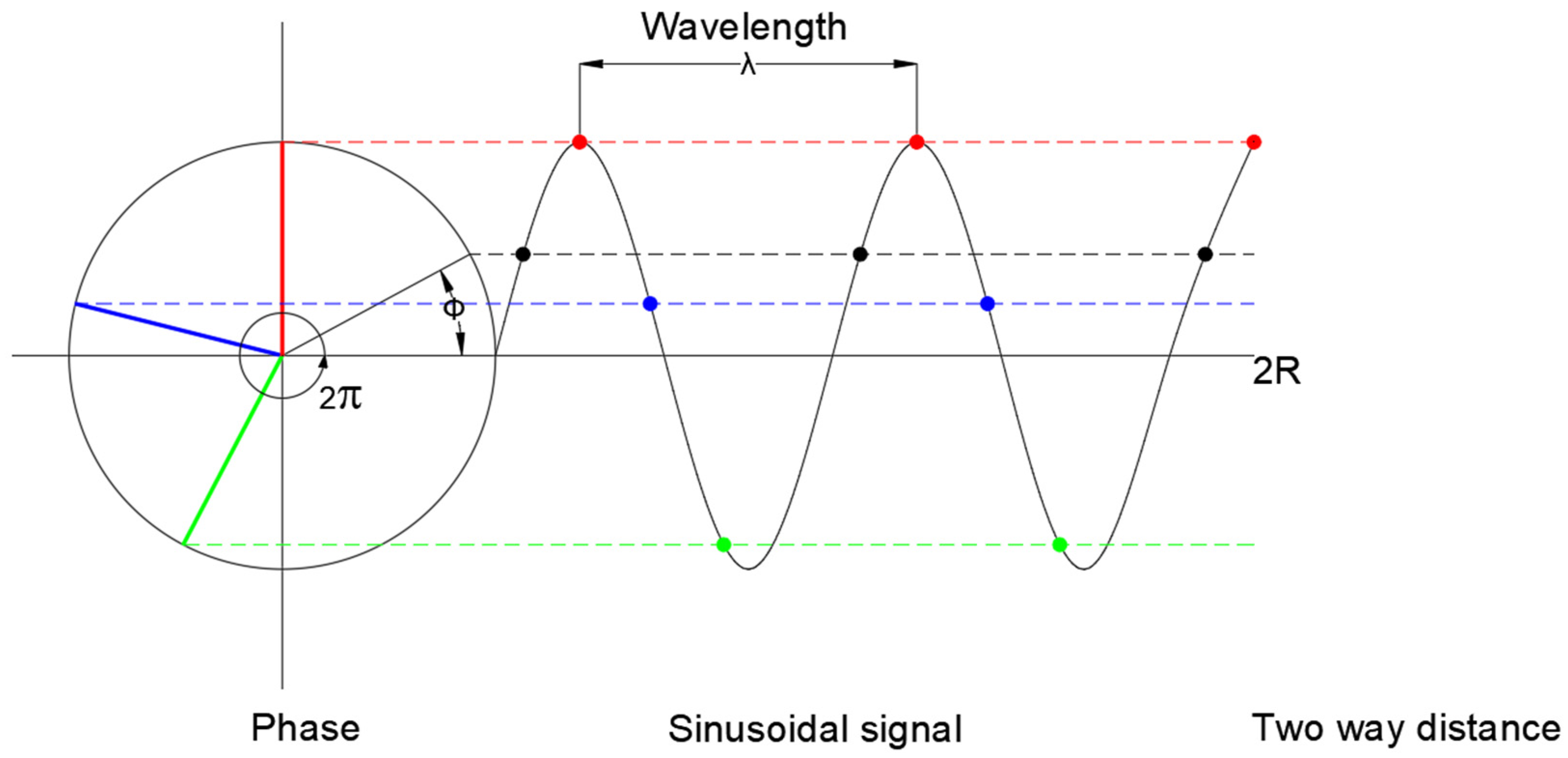
- d = the deformation according to the vertical axis.
- λ = the wavelength used.
- = the phase displacement for each cell between data acquisitions.
- ϴinc = incident angle.
2.4.3. Terrestrial LIDAR Measurements
Materials
Study Period
Data Processing
- Normal diameter: 0.20 m
- Projected diameter: 0.05 m
- Maximum distance: 0.25–1.00 m
- Core points: 0.025 m
3. Results
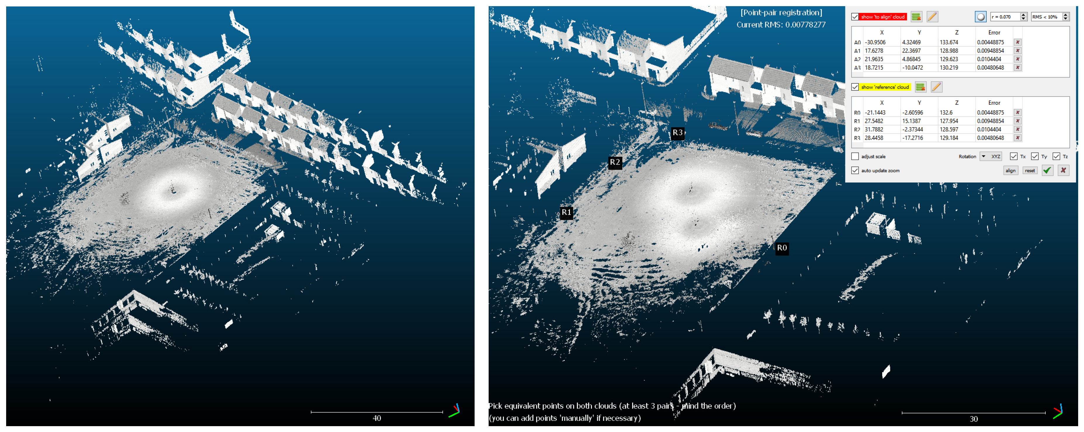
3.1. Comparison of Clouds of Data Points Obtained Using the Terrestrial LIDAR System
- The turning mechanism of the LIDAR system at measuring station 1 on the first (reference) date (Error station R1)
- The turning mechanism of the LIDAR system at measuring station 2 on the first (reference) date (Error station R2)
- The alignment of the clouds of points (measuring stations 1 and 2) on the first (reference) date (RMS CC Reference)
- The turning mechanism of the LIDAR system at measuring station 2 on the first (reference) date (Error station A1)
- The turning mechanism of the LIDAR system at measuring station 2 on the second (aligned) date (Error station A2)
- The alignment of the clouds of data points (measuring stations 1 and 2) on the second (aligned) date (RMS CC Aligned)
- The alignment of the resulting models for the first and second (references vs aligned) dates (RMS CC Compare)
3.2. Differential Inteferometric Analysis of TopSAR Images
- First column shows the dates between deformations.
- Second-column deformation obtained by the differential interferometry method between the cited dates. Green represents a positive deformation, and red a negative deformation. In this figure, the deformation raster has been already corrected in the horizontal plane and in the vertical axis and its value is indicated in the own cell.
- Third-column shows the coherence values obtained using the differential interferometry method between the dates mentioned, vital for making horizontal adjustments and for locating the zero-deformation control points for making vertical adjustments. In this figure the coherence band has been already corrected in the horizontal plane. The values vary between 0 and 1, where 1 (white) represents 100% coherence, and 0 (black) 0% coherence.
- Fourth-column contains the legends for deformation and coherence values.
3.3. Comparison of Differential Interferometry and LIDAR Deformation Measures
4. Discussion
- Concerning the accuracy of measurements, deformation values obtained with both systems were of the order of magnitude of millimetres and tenths of a millimetre, consistent with the erosion observed in the field in the visual inspections, except for the LIDAR results that involve the measurement on 22 May 2017, because of an error in the turning mechanism of LIDAR in position 2. Only two of a total of forty observations surpassed the range of maximum possible error associated with the LIDAR system, both were in periods longer than 12 days (48 and 86 days) and it was for just 0.0003 and 0.0049 m. From 12 to 12 days, there were none exceeding one.
- Concerning the loss of coherence, the results show how coherence is lost as the period between acquisitions increases, so deformation measurements lose accuracy. As exposed above, limiting the time between acquisition to 12 days guarantees that deformation measures are accurate, so the coherence loss corresponds directly to the deformation registered between acquisition, and not to other factors.
5. Conclusions
- The study period of time between acquisition should not exceed 12 days, to guarantee that all the loss of coherence is because of the deformation of the earth’s surface and not from other sources.
- Longer periods can be studied by combining consecutive 12-day steps.
- Small vegetation such as cereal crops does not interfere with InSAR measurements, but larger vegetation such as sunflowers can do so. Verification of the interference of larger vegetation will be the subject of future research.
- The accuracy of the results is highly related to the existence of reliable zero-deformation control points (very high coherence points), used to adjust the deformation in the study area.
- The different soil moisture between acquisitions can alter the deformation measurements by affecting the expansion capability of the clay or the soil dielectric characteristic and its microwave reflecting capability. This effect will be the subject of future research, but meanwhile, it can be avoided by comparing acquisitions with similar soil moisture degrees.
- The effects of soil compaction/decompaction can also affect the measurements because this methodology is based on changes in the earth’s surface but does not consider changes in density. This effect will also be the subject of future research.
Author Contributions
Funding
Data Availability Statement
Acknowledgments
Conflicts of Interest
References
- Seutloali, K.E.; Dube, T.; Sibanda, M. Developments in the Remote Sensing of Soil Erosion in the Perspective of Sub-Saharan Africa. Implications on Future Food Security and Biodiversity. Remote Sens. Appl. Soc. Environ. 2018, 9, 100–106. [Google Scholar] [CrossRef]
- Rhodes, C.J. Soil Erosion, Climate Change and Global Food Security: Challenges and Strategies. Sci. Prog. 2014, 97, 97–153. [Google Scholar] [CrossRef] [PubMed]
- Panagos, P.; Borrelli, P.; Poesen, J.; Ballabio, C.; Lugato, E.; Meusburger, K.; Montanarella, L.; Alewell, C. The New Assessment of Soil Loss by Water Erosion in Europe. Environ. Sci. Policy 2015, 54, 438–447. [Google Scholar] [CrossRef]
- van Leeuwen, C.C.E.; Cammeraat, E.L.H.; de Vente, J.; Boix-Fayos, C. The Evolution of Soil Conservation Policies Targeting Land Abandonment and Soil Erosion in Spain: A Review. Land Use Policy 2019, 83, 174–186. [Google Scholar] [CrossRef]
- Martín-Fernández, L.; Martínez-Núñez, M. An Empirical Approach to Estimate Soil Erosion Risk in Spain. Sci. Total Environ. 2011, 409, 3114–3123. [Google Scholar] [CrossRef] [PubMed]
- Rodrigo-comino, J.; Martínez-hernández, C.; Iserloh, T.; Cerdà, A. Contrasted Impact of Land Abandonment on Soil Erosion in Mediterranean Agriculture Fields. Pedosphere 2018, 28, 617–631. [Google Scholar] [CrossRef]
- Rodriguez-Lloveras, X.; Buytaert, W.; Benito, G. Land Use Can Offset Climate Change Induced Increases in Erosion in Mediterranean Watersheds. Catena 2016, 143, 244–255. [Google Scholar] [CrossRef]
- de Vente, J.; Poesen, J. Predicting Soil Erosion and Sediment Yield at the Basin Scale: Scale Issues and Semi-Quantitative Models. Earth-Sci. Rev. 2005, 71, 95–125. [Google Scholar] [CrossRef]
- Van Oost, K.; Govers, G.; De Alba, S.; Quine, T.A. Tillage Erosion: A Review of Controlling Factors and Implications for Soil Quality. Prog. Phys. Geogr. Earth Environ. 2006, 30, 443–466. [Google Scholar] [CrossRef]
- Wischmeier, W.H.; Smith, D.D. Predicting Rainfall Erosion Losses: A Guide to Conservation Planning (No. 537); Department of Agriculture, Science and Education Administration, U.S. Government Printing Office: Washington DC, USA, 1978.
- Williams, J.R.; Berndt, H.D. Sediment Yield Prediction Based on Watershed Hydrology. Trans. ASAE 1977, 20, 1100–1104. [Google Scholar] [CrossRef]
- Renard, K.G.; Laflen, J.M.; Foster, G.R.; McCool, D.K. The Revised Universal Soil Loss Equation. In Soil Erosion Research Methods; Routledge: New York, NY, USA, 1994; ISBN 978-0-203-73935-8. [Google Scholar]
- Ewing, L.K.; Mitchell, J.K. Overland Flow and Sediment Transport Simulation on Small Plots. Microfiche Collect. 1986, 29, 1572–1581. [Google Scholar]
- Nearing, M.A.; Foster, G.R.; Lane, L.J.; Finkner, S.C. A Process-Based Soil Erosion Model for USDA-Water Erosion Prediction Project Technology. Trans. ASAE 1989, 32, 1587–1593. [Google Scholar] [CrossRef]
- Stroosnijder, L. Measurement of Erosion: Is It Possible? Catena 2005, 64, 162–173. [Google Scholar] [CrossRef]
- Baartman, J.E.M.; Jetten, V.G.; Ritsema, C.J.; de Vente, J. Exploring Effects of Rainfall Intensity and Duration on Soil Erosion at the Catchment Scale Using OpenLISEM: Prado Catchment, SE Spain. Hydrol. Process. 2012, 26, 1034–1049. [Google Scholar] [CrossRef]
- King, C.; Baghdadi, N.; Lecomte, V.; Cerdan, O. The Application of Remote-Sensing Data to Monitoring and Modelling of Soil Erosion. Catena 2005, 62, 79–93. [Google Scholar] [CrossRef]
- Luleva, M.I.; Werff, H.M.A.; van der Meer, F.D.; van der Jetten, V.G. Gaps and Opportunities in the Use of Remote Sensing for Soil Erosion Assessment. Khimiya Chem. Bulg. J. Sci. Educ. 2012, 21, 748–764. [Google Scholar]
- Jetten, V.; Govers, G.; Hessel, R. Erosion Models: Quality of Spatial Predictions. Hydrol. Process. 2003, 17, 887–900. [Google Scholar] [CrossRef]
- Kuhn, N.J.; Greenwood, P.; Fister, W. Chapter 5.1—Use of Field Experiments in Soil Erosion Research. In Developments in Earth Surface Processes; Thornbush, M.J., Allen, C.D., Fitzpatrick, F.A., Eds.; Elsevier: Amsterdam, The Netherlands, 2014; Volume 18, pp. 175–200. [Google Scholar]
- Vrieling, A. Satellite Remote Sensing for Water Erosion Assessment: A Review. Catena 2006, 65, 2–18. [Google Scholar] [CrossRef]
- Bretar, F.; Chauve, A.; Bailly, J.-S.; Mallet, C.; Jacome, A. Terrain Surfaces and 3D Landcover Classification from Small Footprint Full-Waveform Lidar Data: Application to Badlands. Hydrol. Earth Syst. Sci. 2009, 13, 1531–1544. [Google Scholar] [CrossRef]
- Sánchez-Crespo, F.A.; Marques da Silva, J.R.; Gómez-Villarino, M.T.; Gallego, E.; Fuentes, J.M.; García, A.I.; Ayuga, F. Differential Interferometry over Sentinel-1 TopSAR Images as a Tool for Water and Tillage Soil Erosion Analysis. Agronomy 2021, 11, 2075. [Google Scholar] [CrossRef]
- Peter-Contesse, H.; Jäggi, A.; Fernández, J.; Escobar, D.; Ayuga, F.; Arnold, D.; Wermuth, M.; Hackel, S.; Otten, M.; Simons, W.; et al. Sentinel-1A—First Precise Orbit Determination Results. Adv. Space Res. 2017, 60, 879–892. [Google Scholar] [CrossRef]
- Berger, M.; Aschbacher, J. Preface: The Sentinel Missions—New Opportunities for Science. Remote Sens. Environ. 2012, 120, 1–2. [Google Scholar] [CrossRef]
- Osmanoğlu, B.; Sunar, F.; Wdowinski, S.; Cabral-Cano, E. Time Series Analysis of InSAR Data: Methods and Trends. ISPRS J. Photogramm. Remote Sens. 2016, 115, 90–102. [Google Scholar] [CrossRef]
- González, P.J.; Bagnardi, M.; Hooper, A.J.; Larsen, Y.; Marinkovic, P.; Samsonov, S.V.; Wright, T.J. The 2014–2015 Eruption of Fogo Volcano: Geodetic Modeling of Sentinel-1 TOPS Interferometry. Geophys. Res. Lett. 2015, 42, 9239–9246. [Google Scholar] [CrossRef]
- Spreckels, V.; Wegmüller, U.; Strozzi, T.; Musiedlak, J.; Wichlacz, H.C. Detection and Observation of Underground Coal Mining-Induced Surface Deformation with Differential SAR Interferometry. In ISPRS Workshop High Resolution Mapping from Space; University of Hannover: Hannover, Germany, 2001; pp. 227–234. [Google Scholar]
- Halliday, D.; Curtis, A. Seismic Interferometry, Surface Waves and Source Distribution. Geophys. J. Int. 2008, 175, 1067–1087. [Google Scholar] [CrossRef]
- Salvi, S.; Stramondo, S.; Funning, G.J.; Ferretti, A.; Sarti, F.; Mouratidis, A. The Sentinel-1 Mission for the Improvement of the Scientific Understanding and the Operational Monitoring of the Seismic Cycle. Remote Sens. Environ. 2012, 120, 164–174. [Google Scholar] [CrossRef]
- Barboux, C.; Strozzi, T.; Delaloye, R.; Wegmüller, U.; Collet, C. Mapping Slope Movements in Alpine Environments Using TerraSAR-X Interferometric Methods. ISPRS J. Photogramm. Remote Sens. 2015, 109, 178–192. [Google Scholar] [CrossRef]
- Colesanti, C.; Wasowski, J. Investigating Landslides with Space-Borne Synthetic Aperture Radar (SAR) Interferometry. Eng. Geol. 2006, 88, 173–199. [Google Scholar] [CrossRef]
- Squarzoni, C.; Delacourt, C.; Allemand, P. Nine Years of Spatial and Temporal Evolution of the La Valette Landslide Observed by SAR Interferometry. Eng. Geol. 2003, 68, 53–66. [Google Scholar] [CrossRef]
- Anghel, A.; Vasile, G.; Boudon, R.; d’Urso, G.; Girard, A.; Boldo, D.; Bost, V. Combining Spaceborne SAR Images with 3D Point Clouds for Infrastructure Monitoring Applications. ISPRS J. Photogramm. Remote Sens. 2016, 111, 45–61. [Google Scholar] [CrossRef]
- Di Martire, D.; Iglesias, R.; Monells, D.; Centolanza, G.; Sica, S.; Ramondini, M.; Pagano, L.; Mallorquí, J.J.; Calcaterra, D. Comparison between Differential SAR Interferometry and Ground Measurements Data in the Displacement Monitoring of the Earth-Dam of Conza Della Campania (Italy). Remote Sens. Environ. 2014, 148, 58–69. [Google Scholar] [CrossRef]
- Loesch, E.; Sagan, V. SBAS Analysis of Induced Ground Surface Deformation from Wastewater Injection in East Central Oklahoma, USA. Remote Sens. 2018, 10, 283. [Google Scholar] [CrossRef] [Green Version]
- Smith, L.C.; Alsdorf, D.E.; Magilligan, F.J.; Gomez, B.; Mertes, L.A.K.; Smith, N.D.; Garvin, J.B. Caused by the 1996 Skei0arrsandur j / Skulhlaup, Iceland, from Synthetic Aperture Radar Interferometry. Water Resour. Res. 2000, 36, 1583–1594. [Google Scholar] [CrossRef]
- Geudtner, D.; Torres, R.; Snoeij, P.; Davidson, M.; Rommen, B. Sentinel-1 System Capabilities and Applications. In Proceedings of the 2014 IEEE Geoscience and Remote Sensing Symposium, Quebec City, QC, Canada, 13–18 July 2014; pp. 1457–1460. [Google Scholar]
- Zhou, X.; Chang, N.-B.; Li, S. Applications of SAR Interferometry in Earth and Environmental Science Research. Sensors 2009, 9, 1876–1912. [Google Scholar] [CrossRef] [PubMed]
- Eitel, J.U.H.; Höfle, B.; Vierling, L.A.; Abellán, A.; Asner, G.P.; Deems, J.S.; Glennie, C.L.; Joerg, P.C.; LeWinter, A.L.; Magney, T.S.; et al. Beyond 3-D: The New Spectrum of Lidar Applications for Earth and Ecological Sciences. Remote Sens. Environ. 2016, 186, 372–392. [Google Scholar] [CrossRef]
- Li, L.; Nearing, M.A.; Nichols, M.H.; Polyakov, V.O.; Cavanaugh, M.L. Using Terrestrial LiDAR to Measure Water Erosion on Stony Plots under Simulated Rainfall. Earth Surf. Process. Landf. 2020, 45, 484–495. [Google Scholar] [CrossRef]
- Qin, R.; Tian, J.; Reinartz, P. 3D Change Detection—Approaches and Applications. ISPRS J. Photogramm. Remote Sens. 2016, 122, 41–56. [Google Scholar] [CrossRef]
- Touzi, R.; Lopes, A.; Bruniquel, J.; Vachon, P.W. Coherence Estimation for SAR Imagery. IEEE Trans. Geosci. Remote Sens. 1999, 37, 135–149. [Google Scholar] [CrossRef]
- Paloscia, S.; Macelloni, G.; Pampaloni, P.; Sigismondi, S. The Potential of C- and L-Band SAR in Estimating Vegetation Biomass: The ERS-1 and JERS-1 Experiments. IEEE Trans. Geosci. Remote Sens. 1999, 37, 2107–2110. [Google Scholar] [CrossRef]
- Wegner, J.D.; Hänsch, R.; Thiele, A.; Soergel, U. Building Detection From One Orthophoto and High-Resolution InSAR Data Using Conditional Random Fields. IEEE J. Sel. Top. Appl. Earth Obs. Remote Sens. 2011, 4, 83–91. [Google Scholar] [CrossRef]
- Torres, R.; Snoeij, P.; Geudtner, D.; Bibby, D.; Davidson, M.; Attema, E.; Potin, P.; Rommen, B.Ö.; Floury, N.; Brown, M.; et al. GMES Sentinel-1 Mission. Remote Sens. Environ. 2012, 120, 9–24. [Google Scholar] [CrossRef]
- Koch, B. Status and Future of Laser Scanning, Synthetic Aperture Radar and Hyperspectral Remote Sensing Data for Forest Biomass Assessment. ISPRS J. Photogramm. Remote Sens. 2010, 65, 581–590. [Google Scholar] [CrossRef]
- Tamm, T.; Zalite, K.; Voormansik, K.; Talgre, L. Relating Sentinel-1 Interferometric Coherence to Mowing Events on Grasslands. Remote Sens. 2016, 8, 802. [Google Scholar] [CrossRef]
- Wang, Y.; Shi, H.; Zhang, Y.; Zhang, D. Automatic Registration of Laser Point Cloud Using Precisely Located Sphere Targets. J. Appl. Remote Sens. 2014, 8, 083588. [Google Scholar] [CrossRef]
- CloudCompare—Documentation. Available online: https://www.cloudcompare.org/doc/ (accessed on 24 November 2022).
- Theiler, P.W.; Wegner, J.D.; Schindler, K. Keypoint-Based 4-Points Congruent Sets—Automated Marker-Less Registration of Laser Scans. ISPRS J. Photogramm. Remote Sens. 2014, 96, 149–163. [Google Scholar] [CrossRef]
- Ferretti, A.; Monti-Guarnieri, A.; Prati, C.; Rocca, F. InSAR Principles: Guidelines for SAR Interferometry Processing and Interpretation (ESA TM-19). Available online: https://www.esa.int/About_Us/ESA_Publications/InSAR_Principles_Guidelines_for_SAR_Interferometry_Processing_and_Interpretation_br_ESA_TM-19 (accessed on 24 November 2022).
- Martone, M.; Bräutigam, B.; Rizzoli, P.; Gonzalez, C.; Bachmann, M.; Krieger, G. Coherence Evaluation of TanDEM-X Interferometric Data. ISPRS J. Photogramm. Remote Sens. 2012, 73, 21–29. [Google Scholar] [CrossRef]
- Engdahl, M.; Minchella, A.; Marinkovic, P.; Veci, L.; Lu, J. NEST: An Esa Open Source Toolbox for Scientific Exploitation of SAR Data. In Proceedings of the 2012 IEEE International Geoscience and Remote Sensing Symposium, Munich, Germany, 22–27 July 2012; pp. 5322–5324. [Google Scholar]
- Zuhlke, M.; Fomferra, N.; Brockmann, C.; Peters, M.; Veci, L.; Malik, J.; Regner, P. SNAP (Sentinel Application Platform) and the ESA Sentinel 3 Toolbox. In Proceedings of the Sentinel-3 for Science Workshop, Venice, Italy, 2–5 June 2015; Ouwehand, L., Ed.; Volume 734, p. 21, ISBN 978-92-9221-298-8. [Google Scholar]
- Chen, C.W.; Zebker, H.A. Network Approaches to Two-Dimensional Phase Unwrapping: Intractability and Two New Algorithms. JOSA A 2000, 17, 401–414. [Google Scholar] [CrossRef]
- Chen, C.W.; Zebker, H.A. Two-Dimensional Phase Unwrapping with Use of Statistical Models for Cost Functions in Nonlinear Optimization. JOSA A 2001, 18, 338–351. [Google Scholar] [CrossRef]
- Chen, C.W.; Zebker, H.A. Phase Unwrapping for Large SAR Interferograms: Statistical Segmentation and Generalized Network Models. IEEE Trans. Geosci. Remote Sens. 2002, 40, 1709–1719. [Google Scholar] [CrossRef]
- Monti Guarnieri, A.; Mancon, S.; Tebaldini, S. Sentinel-1 Precise Orbit Calibration and Validation. In Proceedings of the Fringe 2015: Advances in the Science and Applications of SAR Interferometry and Sentinel-1 InSAR Workshop, Paris, France, 1 May 2015. [Google Scholar]
- De Zan, F.; Monti Guarnieri, A. TOPSAR: Terrain Observation by Progressive Scans. IEEE Trans. Geosci. Remote Sens. 2006, 44, 2352–2360. [Google Scholar] [CrossRef]
- Yagüe-Martínez, N.; Prats-Iraola, P.; Rodríguez González, F.; Brcic, R.; Shau, R.; Geudtner, D.; Eineder, M.; Bamler, R. Interferometric Processing of Sentinel-1 TOPS Data. IEEE Trans. Geosci. Remote Sens. 2016, 54, 2220–2234. [Google Scholar] [CrossRef]
- Goldstein, R.M.; Werner, C.L. Radar Interferogram Filtering for Geophysical Applications. Geophys. Res. Lett. 1998, 25, 4035–4038. [Google Scholar] [CrossRef] [Green Version]
- Small, D.; Pasquali, P.; Fuglistaler, S. A Comparison of Phase to Height Conversion Methods for SAR Interferometry. In Proceedings of the IGARSS ’96. 1996 International Geoscience and Remote Sensing Symposium, Lincoln, NE, USA, 31 May 1996; Volume 1, pp. 342–344. [Google Scholar]
- Richards, M.A. A Beginner’s Guide to Interferometric SAR Concepts and Signal Processing [AESS Tutorial IV]. IEEE Aerosp. Electron. Syst. Mag. 2007, 22, 5–29. [Google Scholar] [CrossRef]
- Rodriguez-Cassola, M.; Prats-Iraola, P.; De Zan, F.; Scheiber, R.; Reigber, A.; Geudtner, D.; Moreira, A. Doppler-Related Distortions in TOPS SAR Images. IEEE Trans. Geosci. Remote Sens. 2015, 53, 25–35. [Google Scholar] [CrossRef]
- Lague, D.; Brodu, N.; Leroux, J. Accurate 3D Comparison of Complex Topography with Terrestrial Laser Scanner: Application to the Rangitikei Canyon (N-Z). ISPRS J. Photogramm. Remote Sens. 2013, 82, 10–26. [Google Scholar] [CrossRef]
- Brodu, N.; Lague, D. 3D Terrestrial Lidar Data Classification of Complex Natural Scenes Using a Multi-Scale Dimensionality Criterion: Applications in Geomorphology. ISPRS J. Photogramm. Remote Sens. 2012, 68, 121–134. [Google Scholar] [CrossRef]
- Weinmann, M.; Jutzi, B.; Hinz, S.; Mallet, C. Semantic Point Cloud Interpretation Based on Optimal Neighborhoods, Relevant Features and Efficient Classifiers. ISPRS J. Photogramm. Remote Sens. 2015, 105, 286–304. [Google Scholar] [CrossRef]
- Demantké, J.; Mallet, C.; David, N.; Vallet, B. Dimensionality based scale selection in 3d lidar point clouds. Int. Arch. Photogramm. Remote Sens. Spat. Inf. Sci. 2012, XXXVIII-5/W12, 97–102. [Google Scholar] [CrossRef] [Green Version]
- Schenkelberg, F. Root Sum Squared Tolerance Analysis Method. Root Sum Squared Method. Accendo Reliability, 2017. Available online: https://accendoreliability.com/root-sum-squared-tolerance-analysis-method/ (accessed on 13 August 2017).


| Date | Satellite Sentinel | Orbit | Local Time |
|---|---|---|---|
| 28 April 2017 | S-1A | Ascending | 19:10–19:12 |
| 10 May 2017 | S-1A | Ascending | 19:10–19:12 |
| 22 May 2017 | S-1A | Ascending | 19:10–19:12 |
| 3 June 2017 | S-1A | Ascending | 19:10–19:12 |
| 15 June 2017 | S-1A | Ascending | 19:10–19:12 |
| 27 June 2017 | S-1A | Ascending | 19:10–19:12 |
| 9 July 2017 | S-1A | Ascending | 19:10–19:12 |
| 15 July 2017 | S-1B | Ascending | 19:10–19:11 |
| 30 December 2017 | S-1B | Ascending | 19:10–19:11 |
| 11 January 2018 | S-1B | Ascending | 19:10–19:11 |
| Vertical Adjustment (m) | |||
|---|---|---|---|
| Dates | Control Point Value | Control Point Coherence | |
| 28 April 2017 | 10 May 2017 | −0.02574 | 0.98794 |
| 28 April 2017 | 22 May 2017 | −0.05999 | 0.97597 |
| 28 April 2017 | 15 June 2017 | −0.06752 | 0.96981 |
| 28 April 2017 | 9 July 2017 | −0.16464 | 0.93012 |
| 10 May 2017 | 10 May 2017 | −0.03508 | 0.97794 |
| 22 May 2017 | 3 June 2017 | 0.01051 | 0.96236 |
| 3 June 2017 | 15 June 2017 | −0.03450 | 0.96150 |
| 15 June 2017 | 27 June 2017 | 0.03143 | 0.98654 |
| 27 June 2017 | 9 July 2017 | −0.05201 | 0.98177 |
| 30 December 2017 | 11 January 2018 | −0.00314 | 0.99392 |
| Date | Measured Using: |
|---|---|
| 23 March 2017 | 1 measuring station and 4 spheres. Radial de-correlation. DATA REJECTED |
| 29 March 2017 | 1 station and 4 spheres. Radial de-correlation. DATA REJECTED |
| 4 April 2017 | 1 station and 4 spheres. Radial de-correlation. DATA REJECTED |
| 10 April 2017 | 1 station and 4 spheres. Radial de-correlation. DATA REJECTED |
| 16 April 2017 | 1 station and 4 spheres. Radial de-correlation. DATA REJECTED |
| 28 April 2017 | 2 stations and 4 spheres (2 clouds per model) |
| 4 May 2017 | 2 stations and 4 spheres (2 clouds per model) |
| 10 May 2017 | 2 stations and 4 spheres (2 clouds per model) |
| 16 May 2017 | 2 stations and 4 spheres (2 clouds per model) |
| 22 May 2017 | 2 stations and 4 spheres (2 clouds per model) |
| 28 May 2017 | 2 stations and 4 spheres (2 clouds per model) |
| 3 June 2017 | 2 stations and 4 spheres (2 clouds per model) |
| 9 June 2017 | 2 stations and 4 spheres (2 clouds per model) |
| 15 June 2017 | 2 stations and 4 spheres (2 clouds per model) |
| 21 June 2017 | 2 stations and 4 spheres (2 clouds per model) |
| 27 June 2017 | 2 stations and 4 spheres (2 clouds per model) |
| 3 July 2017 | 2 stations and 4 spheres (2 clouds per model) |
| 9 July 2017 | 2 stations and 4 spheres (2 clouds per model) |
| 15 July 2017 | Repeated 16 July 2017 due to error in the memory card. 2 stations and 4 spheres (2 clouds per model) |
| 30 December 2017 | 2 stations and 6 spheres (2 clouds per model) |
| 5 January 2018 | No data taken due to rain |
| 11 January 2018 | 2 stations and 6 spheres (2 clouds per model) |
| Lidar Estimated Errors and Deformation Measures (m) | ||||||||||||||||||
|---|---|---|---|---|---|---|---|---|---|---|---|---|---|---|---|---|---|---|
| Reference | Aligned | Error Position Reference Base | Error Position Aligned Base | EP Total | RMS | Max. Possible Error | Deformation Measures | |||||||||||
| EP R1 | EP R2 | EP Ref. | EP A1 | EP A4 | EP Aligned | RMS CC Ref. | RMS CC Aligned | RMS CC Compare | RMS CC Total | AL | BL | CL | DL | Global (A B C D)L | ||||
| Absolute | R1 | R2 | * | A1 | A2 | ** | *** | RMSR | RMSA | RMSC | **** | ***** | AL | BL | CL | DL | ||
| 28 April 2017 | 10 May 2017 | 0.0021 | 0.0039 | 0.0031 | 0.0024 | 0.0022 | 0.0023 | 0.0027 | 0.0068 | 0.0073 | 0.0110 | 0.0085 | 0.0090 | −0.0003 | −0.0029 | 0.0017 | 0.0016 | 0.0000 |
| 28 April 2017 | 22 May 2017 | 0.0021 | 0.0039 | 0.0031 | 0.0022 | 0.0486 | 0.0344 | 0.0244 | 0.0068 | 0.0125 | 0.0093 | 0.0098 | 0.0263 | −0.0122 | −0.0136 | −0.0043 | −0.0018 | −0.0080 |
| 28 April 2017 | 15 June 2017 | 0.0021 | 0.0039 | 0.0031 | 0.0019 | 0.0018 | 0.0018 | 0.0025 | 0.0068 | 0.0088 | 0.0083 | 0.0080 | 0.0084 | 0.0025 | −0.0033 | 0.0132 | −0.0012 | 0.0028 |
| 28 April 2017 | 9 July 2017 | 0.0021 | 0.0039 | 0.0031 | 0.0044 | 0.0022 | 0.0035 | 0.0033 | 0.0068 | 0.0083 | 0.0117 | 0.0091 | 0.0097 | −0.0024 | −0.0075 | 0.0101 | 0.0026 | 0.0007 |
| Incremental | ||||||||||||||||||
| 28 April 2017 | 10 May 2017 | 0.0021 | 0.0039 | 0.0031 | 0.0022 | 0.0024 | 0.0023 | 0.0027 | 0.0068 | 0.0073 | 0.0110 | 0.0085 | 0.0090 | −0.0003 | −0.0029 | 0.0017 | 0.0016 | 0.0000 |
| 10 May 2017 | 22 May 2017 | 0.0022 | 0.0024 | 0.0023 | 0.0022 | 0.0486 | 0.0344 | 0.0244 | 0.0073 | 0.0125 | 0.0098 | 0.0101 | 0.0264 | −0.0119 | −0.0112 | −0.0057 | −0.0032 | −0.0080 |
| 22 May 2017 | 20170603 | 0.0022 | 0.0486 | 0.0344 | 0.0041 | 0.0019 | 0.0032 | 0.0244 | 0.0125 | 0.0090 | 0.0102 | 0.0107 | 0.0267 | 0.0191 | 0.0153 | 0.0170 | −0.0008 | 0.0127 |
| 3 June 2017 | 15 June 2017 | 0.0041 | 0.0019 | 0.0032 | 0.0019 | 0.0018 | 0.0018 | 0.0026 | 0.0090 | 0.0088 | 0.0083 | 0.0087 | 0.0091 | −0.0040 | −0.0039 | 0.0012 | 0.0014 | −0.0013 |
| 15 June 2017 | 27 June 2017 | 0.0019 | 0.0018 | 0.0018 | 0.0021 | 0.0021 | 0.0021 | 0.0020 | 0.0088 | 0.0109 | 0.0083 | 0.0094 | 0.0096 | −0.0013 | −0.0008 | −0.0014 | −0.0010 | −0.0011 |
| 27 June 2017 | 9 July 2017 | 0.0021 | 0.0021 | 0.0021 | 0.0044 | 0.0022 | 0.0035 | 0.0029 | 0.0109 | 0.0124 | 0.0111 | 0.0115 | 0.0118 | −0.0044 | −0.0035 | −0.0023 | 0.0048 | −0.0014 |
| 30 December 2017 | 11 January 2018 | 0.0025 | 0.0021 | 0.0023 | 0.0020 | 0.0020 | 0.0020 | 0.0021 | 0.0101 | 0.0053 | 0.0061 | 0.0075 | 0.0078 | −0.0016 | 0.0017 | 0.0027 | −0.0018 | 0.0002 |
| INSAR TOPSAR Measures (m) | ||||||||||||
|---|---|---|---|---|---|---|---|---|---|---|---|---|
| Reference | Aligned | Vertical Error Adjustment (m) | Original Measure (m) | Corrected Measure (m) | ||||||||
| Control Point Value | Control Point Coherence | A | B | C | D | A’ | B’ | C’ | D’ | Global A’B’C’D’ | ||
| Absolute | x | A | B | C | D | A’ = (A − x) | B’ = (B − x) | C’ = (C − x) | D’ = (D − x) | |||
| 28 April 2017 | 10 May 2017 | −0.02574 | 0.98794 | −0.02383 | −0.02348 | −0.02335 | −0.02358 | 0.00192 | 0.00226 | 0.00239 | 0.00216 | 0.00218 |
| 28 April 2017 | 22 May 2017 | −0.05999 | 0.97597 | −0.05749 | −0.05854 | −0.05835 | −0.05815 | 0.00250 | 0.00145 | 0.00164 | 0.00184 | 0.00186 |
| 28 April 2017 | 15 June 2017 | −0.06752 | 0.96981 | −0.06637 | −0.06718 | −0.06762 | −0.06716 | 0.00114 | 0.00033 | −0.00010 | 0.00035 | 0.00043 |
| 28 April 2017 | 9 July 2017 | −0.16464 | 0.93012 | −0.16202 | −0.16218 | −0.16165 | −0.16452 | 0.00262 | 0.00246 | 0.00298 | 0.00012 | 0.00204 |
| Incremental | ||||||||||||
| 28 April 2017 | 10 May 2017 | −0.02574 | 0.98794 | −0.02383 | −0.02348 | −0.02335 | −0.02358 | 0.00192 | 0.00226 | 0.00239 | 0.00216 | 0.00218 |
| 10 May 2017 | 22 May 2017 | −0.03508 | 0.97794 | −0.03582 | −0.03584 | −0.03493 | −0.03517 | −0.00074 | −0.00076 | 0.00014 | −0.00010 | −0.00036 |
| 22 May 2017 | 3 June 2017 | 0.01051 | 0.96236 | 0.01247 | 0.01243 | 0.01185 | 0.01163 | 0.00196 | 0.00191 | 0.00133 | 0.00112 | 0.00158 |
| 3 June 2017 | 15 June 2017 | −0.03450 | 0.96150 | −0.03636 | −0.03106 | −0.03679 | −0.03574 | −0.00186 | 0.00344 | −0.00229 | −0.00124 | −0.00049 |
| 15 June 2017 | 27 June 2017 | 0.03143 | 0.98654 | 0.03267 | 0.03113 | 0.03258 | 0.03207 | 0.00125 | −0.00030 | 0.00115 | 0.00064 | 0.00068 |
| 27 June 2017 | 9 July 2017 | −0.05201 | 0.98177 | −0.04979 | −0.05145 | −0.05039 | −0.05052 | 0.00222 | −0.00056 | 0.00162 | 0.00149 | 0.00147 |
| 30 December 2017 | 11 January 2018 | −0.00314 | 0.99392 | −0.00244 | −0.00211 | −0.00341 | −0.00438 | 0.00070 | 0.00103 | −0.00027 | −0.00124 | 0.00006 |
| InSAR TopSAR Measurements vs. LIDAR Measurements (m) | |||||||
|---|---|---|---|---|---|---|---|
| Reference | Aligned | Permissible Range (LIDAR Max. Error) | Difference between LIDAR and InSAR | ||||
| ΔA | ΔB | ΔC | ΔD | Global Difference (A B C D) | |||
| Absolute | ΔA = (A’ − AL) | ΔB = (B’ − BL) | ΔC = (C’ − CL) | ΔD = (D’ − DL) | |||
| 28 April 2017 | 10 May 2017 | 0.0090 | 0.0022 | 0.0052 | 0.0007 | 0.0006 | 0.0022 |
| 28 April 2017 | 22 May 2017 | 0.0263 | 0.0147 | 0.0151 | 0.0060 | 0.0036 | 0.0098 |
| 28 April 2017 | 15 June 2017 | 0.0084 | 0.0014 | 0.0036 | 0.0133 | 0.0015 | 0.0024 |
| 28 April 2017 | 09 July 2017 | 0.0097 | 0.0050 | 0.0100 | 0.0071 | 0.0025 | 0.0014 |
| Incremental | |||||||
| 28 April 2017 | 10 May 2017 | 0.0090 | 0.0022 | 0.0052 | 0.0007 | 0.0006 | 0.0022 |
| 10 May 2017 | 22 May 2017 | 0.0264 | 0.0111 | 0.0104 | 0.0059 | 0.0031 | 0.0076 |
| 22 May 2017 | 03 June 2017 | 0.0267 | 0.0171 | 0.0134 | 0.0157 | 0.0019 | 0.0111 |
| 03 June 2017 | 15 June 2017 | 0.0091 | 0.0021 | 0.0073 | 0.0035 | 0.0026 | 0.0008 |
| 15 June 2017 | 27 June 2017 | 0.0096 | 0.0025 | 0.0005 | 0.0026 | 0.0017 | 0.0018 |
| 27 June 2017 | 09 July 2017 | 0.0118 | 0.0067 | 0.0041 | 0.0039 | 0.0033 | 0.0028 |
| 30 December 2017 | 11 January 2018 | 0.0078 | 0.0023 | 0.0007 | 0.0029 | 0.0005 | 0.0002 |
Disclaimer/Publisher’s Note: The statements, opinions and data contained in all publications are solely those of the individual author(s) and contributor(s) and not of MDPI and/or the editor(s). MDPI and/or the editor(s) disclaim responsibility for any injury to people or property resulting from any ideas, methods, instructions or products referred to in the content. |
© 2023 by the authors. Licensee MDPI, Basel, Switzerland. This article is an open access article distributed under the terms and conditions of the Creative Commons Attribution (CC BY) license (https://creativecommons.org/licenses/by/4.0/).
Share and Cite
Sánchez-Crespo, F.A.; Gómez-Villarino, M.T.; Gallego, E.; Fuentes, J.M.; García, A.I.; Ayuga, F. Monitoring of Water and Tillage Soil Erosion in Agricultural Basins, a Comparison of Measurements Acquired by Differential Interferometric Analysis of Sentinel TopSAR Images and a Terrestrial LIDAR System. Land 2023, 12, 408. https://0-doi-org.brum.beds.ac.uk/10.3390/land12020408
Sánchez-Crespo FA, Gómez-Villarino MT, Gallego E, Fuentes JM, García AI, Ayuga F. Monitoring of Water and Tillage Soil Erosion in Agricultural Basins, a Comparison of Measurements Acquired by Differential Interferometric Analysis of Sentinel TopSAR Images and a Terrestrial LIDAR System. Land. 2023; 12(2):408. https://0-doi-org.brum.beds.ac.uk/10.3390/land12020408
Chicago/Turabian StyleSánchez-Crespo, Francisco A., María Teresa Gómez-Villarino, Eutiquio Gallego, José M. Fuentes, Ana I. García, and Francisco Ayuga. 2023. "Monitoring of Water and Tillage Soil Erosion in Agricultural Basins, a Comparison of Measurements Acquired by Differential Interferometric Analysis of Sentinel TopSAR Images and a Terrestrial LIDAR System" Land 12, no. 2: 408. https://0-doi-org.brum.beds.ac.uk/10.3390/land12020408