Modeling Land Use and Land Cover Changes and Their Effects on Biodiversity in Central Kalimantan, Indonesia

Abstract

Land use and land cover (LULC) change causes biodiversity decline through loss, alteration, and fragmentation of habitats. There are uncertainties on how LULC will change in the future and the effect of such change on biodiversity. In this paper we applied the Land Change Modeler (LCM) and Integrated Valuation of Ecosystem Services and Tradeoffs (InVEST) Scenario Generator tool to develop three spatially explicit LULC future scenarios from 2015 to 2030 in the Pulang Pisau district of Central Kalimantan, Indonesia. The district is experiencing a rapid loss of biodiversity as a result of unprecedented LULC changes. Further, we used the InVEST Habitat Quality model to map habitat quality as a proxy to biodiversity in each of the scenarios. We find habitat quality decline is largest in a scenario where past trends of LULC change continue, followed by a scenario with planned agricultural expansion. Alternately, a conservation-oriented scenario results in significant improvements in habitat quality for biodiversity. This information can support in developing appropriate land use policy for biodiversity conservation in Indonesia.

1. Introduction

Human societies have been built on using biodiversity and thus value biodiversity for its intrinsic worth and its contribution toward the production of various ecosystem goods and services (ESs) that contribute to human well-being [1,2]. Biodiversity also stabilizes the delivery of ecosystem services through time [3,4]. However, many activities crucial for subsistence living have led to biodiversity loss [2,5]. Among these activities is the human-induced land use and land cover (LULC) change that causes biodiversity decline through the loss, alteration, and fragmentation of habitats [6,7]. Land use has been identified as the leading driver of global biodiversity change by the year 2100 [8]. This is of concern not only for the ecosystems but also for human well-being, as loss of biodiversity also translates to loss of many important ecosystem goods and services. In the future, the world will face new interconnected land use challenges resulting from the anticipated increased in the demand for goods and services from limited land resources. [9]. Land managers and policymakers are increasingly concerned about how to improve land management with a minimum impact on biodiversity and corresponding ecosystems. However, there is a significant gap in our understanding of the spatial and temporal ecology of biodiversity and ecosystem goods and services. This, in turn, impedes our ability to manage landscapes sustainably [10]. Several global initiatives such as the Millenium Ecosystem Assessment (MA), the Intergovernmental Panel on Biodiversity and the Ecosystem Services (IPBES), and The Economics of Ecosystems and Biodiversity (TEEB) have emphasized the need to assess biodiversity and ecosystems to develop strategies for promoting human and ecological welfare [2,11,12].

In this context, the notion of developing LULC scenarios with a subsequent assessment of changes in biodiversity and ecosystem services is gaining momentum. Scenarios provide insights into the future through visual representations based on assumptions or data trajectories. The information on the potential outcomes of alternative scenarios can be an important tool while making difficult policy decisions [13]. These scenarios can communicate associated benefits and tradeoffs to policymakers and land planners and managers [10,14,15,16]. They show that spatial and temporal changes in LULC can be used to assess biodiversity and ESs and the trade-offs that occur between different land uses. Advances in modeling software systems have made it possible to develop future scenarios and map biodiversity from different land use scenarios [17,18,19]. A wide range of approaches are available to model LULC change scenarios ranging from machine learning approaches, cellular approaches, economic approaches, agent-based approaches, and hybrid approaches [20]. While measuring and valuing biodiversity has progressed [21], it remains a challenging task [8,12]. One way to assess biodiversity is to spatially model habitat quality [22]. However, this process requires incorporating many properties of the ecosystem, which are complex. Further, traditional terrestrial data collection methods have proved to be extremely time and resource-consuming [22,23,24]. There are also accessibility difficulties in many valuable habitats [22]. In addressing these challenges, models based on geographic information systems (GIS) offer varying strengths and weaknesses to the processing of LULC changes and biodiversity [20,25]. The methods for habitat quality analysis have evolved into an active community with wide-scale operational applications [26].

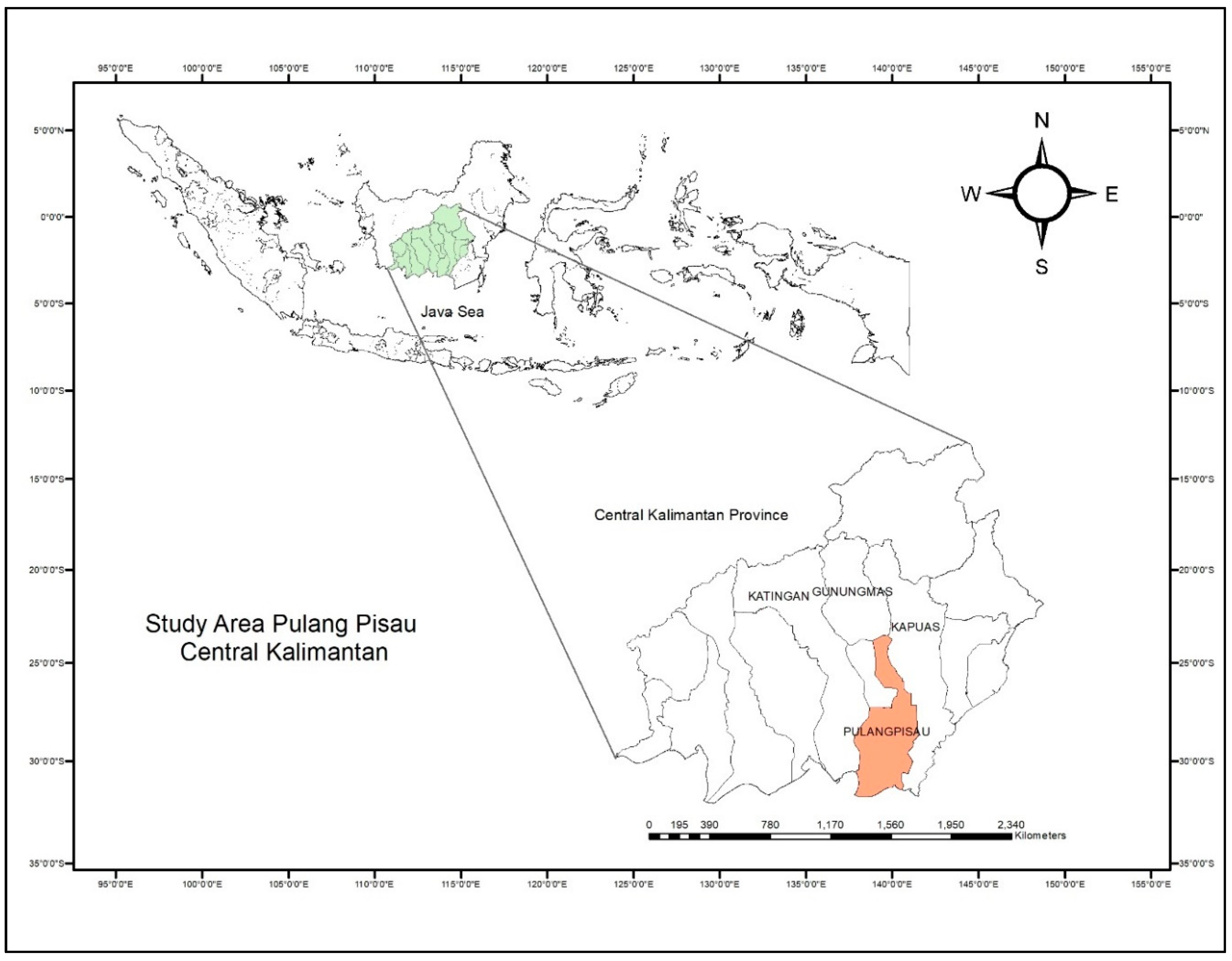
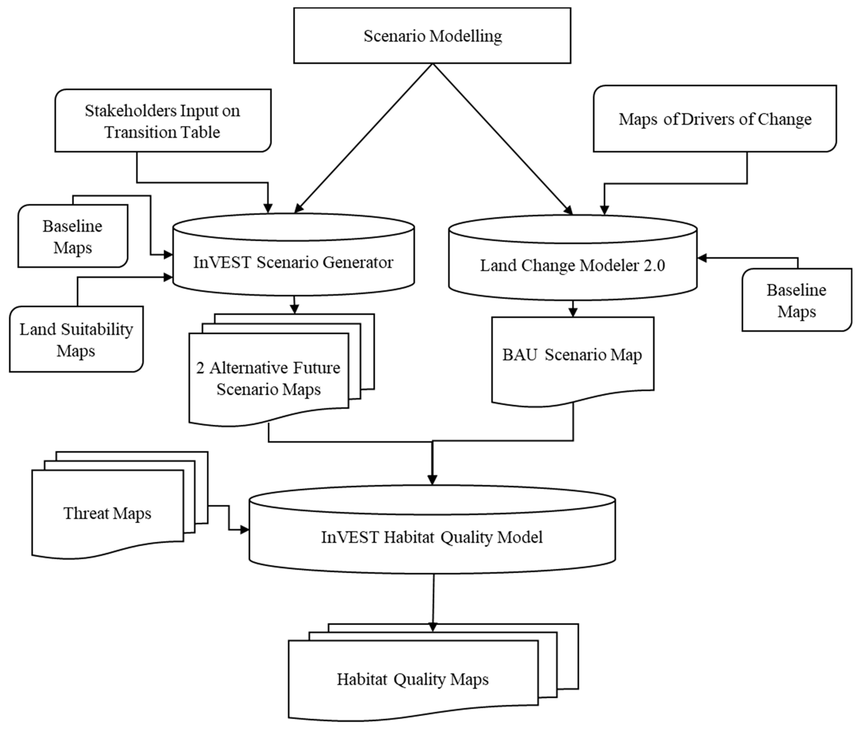
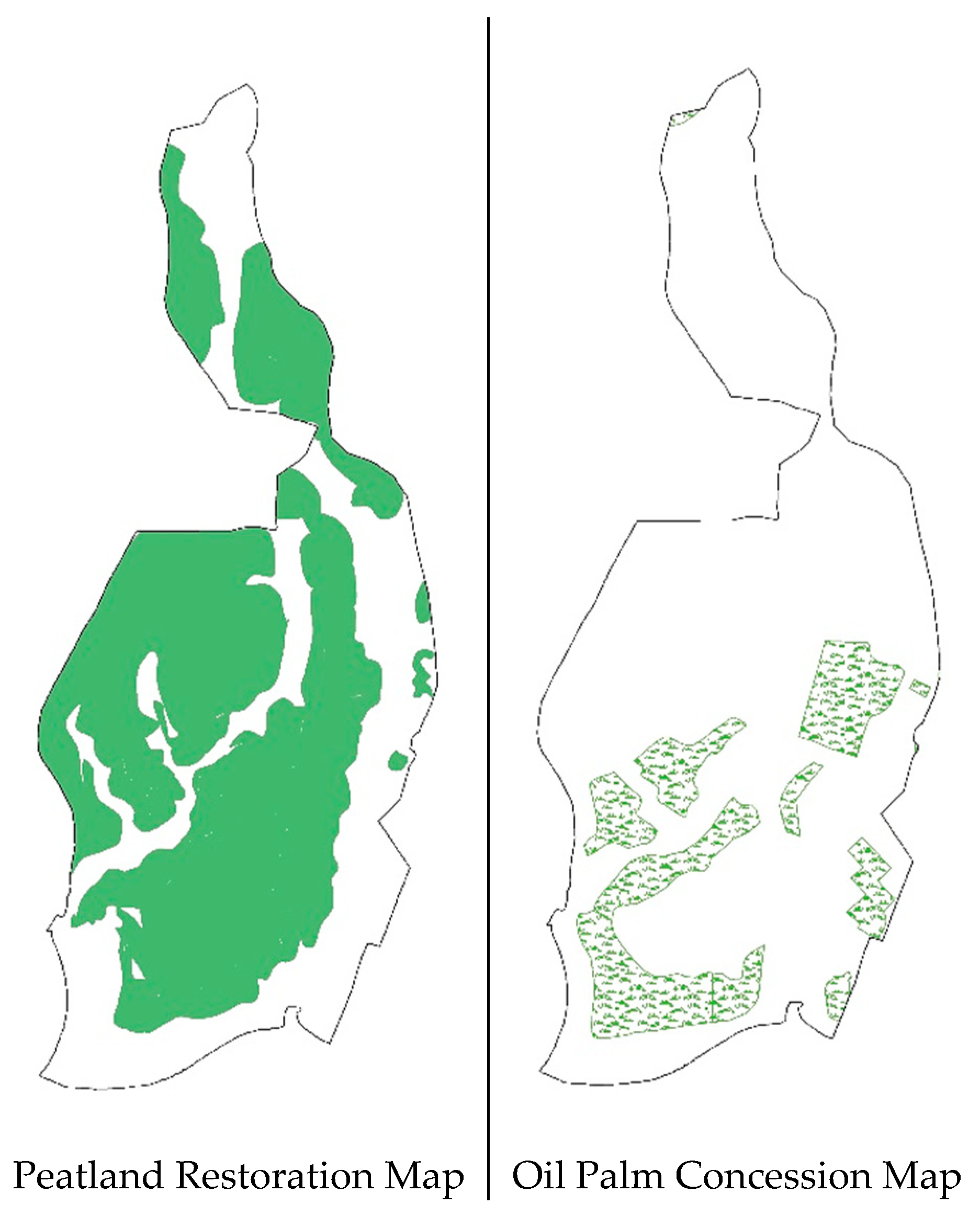
Many studies have modeled LULC changes and their effects on biodiversity. However, in developing countries like Indonesia, with usually limited data availability, modeling approaches are in their infancy. Moreover, no study has explicitly focused on LULC changes and biodiversity at both the local and landscape scales in Indonesia. This study is the first application of GIS-based integrated modeling tools in the assessment of biodiversity at a landscape scale in the district. In this paper, we use the Land Change Modeler (LCM) and InVEST (Integrated Valuation of Ecosystem Services and Tradeoffs) Scenario Generator to develop alternative LULC scenarios. Further, we used the InVEST Habitat Quality model to assess habitat quality under each of the scenarios. The specific aim was to develop three alternative LULC scenarios and assess the spatial distribution of biodiversity under each of them. The Pulang Pisau district of Central Kalimantan province in Indonesia was used as a case study. Central Kalimantan hosts a wide diversity of flora and fauna [27]. However, the rich biodiversity in the province of Kalimantan is declining at an unprecedented rate due to rapid LULC changes, mainly forest conversion caused by land-based economic development (mainly the establishment of oil palm plantations) [28]. Oil palm expansion and deforestation in Central Kalimantan is one of the highest in Indonesia [29] During the period of 1990–2005, at least 56% of oil palm expansion in Indonesia came from forest conversion [30]. The comparison of the land cover map of Pulang Pisau between 2006 and 2015 shows that about 15% of the converted forests during this time came from new oil palm plantations. In the future, further economic development poses an additional threat to the biodiversity in the district. The information on the impact of possible LULC changes on biodiversity will help policymakers formulate appropriate land use policy.

2. Methods

2.1.Study Area

The district of Pulang Pisau is in the southeast part of Central Kalimantan province, Indonesia. The district is bordered by Katingan district in the west, Kapuas district in the east, Gunung Mas district in the north, and the Java Sea in the south (Figure 1). The geographic position is between 113°30′00″–114°15′00″ East longitude and 1°32′00″–3°28′00″ South Latitude [31]. The district’s tropical climate is characterized by high relative humidity (75–87.4%) and a temperature range of 20 °C to 35.8 °C. The topography ranges from coastal and peat swamps in the south to highlands in the north. Almost 30% of the total land area is covered by peat swamp forests. The ecosystem’s carbon storage potential and rich biodiversity makes it the most important land cover type for conservation in the district. The typical land use pattern in the district is oil palm plantations and farmland, each covering almost 10% of the district area.

A significant amount of the district’s peatlands is degraded due to human activities such as drainage and land conversion [32]. However, the remaining pristine peat swamp forests sustain high biodiversity. The rich biodiversity of the district includes many indigenous species of trees along with 63 recorded mammal species (including nine primate species) [33]. Sebangau National Park protects almost a quarter of Pulang Pisau district. The park provides a natural habitat to a variety of endangered species, such as the orangutan (Pongo pygmaeus), clouded leopard (Neofelis diardi), probiscus monkey (Nasalis larvatus), gibbon (Hylobates spp.), malayan sun bear (Helarctos malayanus), hornbills (Rhinoplax vigil, Buceros spps) [27,34,35].

2.2. Models and Tools

We used three spatially explicit modeling softwares and ArcGIS 10.3 to prepare and process the geospatial data. Clark Lab’s Land Change Modeler for ArcGIS Software Extension (2.0) (LCM) and an open-source Integrated Valuation of Ecosystem Services and Tradeoffs (InVEST) The Rule-Based Scenario Generator version 3.4.0 (https://www.naturalcapitalproject.org/invest/) was used to develop LULC scenarios for the year 2030. LCM uses historical datasets and drivers of change variables in the form of maps. The InVEST Scenario Generator uses data on the land use transition patterns and land suitability factors to develop future maps. Finally, the InVEST Habitat Quality model was used to map habitat quality as a proxy for biodiversity. InVEST Habitat Quality uses different data parameters; impact and distance of threats and sensitivity and accessibility of habitats to threats. The conceptual framework of the study is shown in Figure 2.

2.2.1. Scenario Modeling

We defined three LULC scenarios and extrapolated them to the year 2030: business-as-usual (BAU), development, and conservation. In the BAU scenario, we assumed the continuation of past LULC transitions. We compared and analyzed LULC maps produced by the Ministry of Environment and Forestry of Indonesia in 2006 and 2015 (Appendix A). The maps were produced by digitation processes and visual interpretation using Landsat data with a spatial resolution of 30 m. LCM showed significant LULC change in the district. Forest cover decreased by almost 22% and was converted to open lands (60%), swampy bushes (35%), and oil palm plantations (15%). This suggests increasing levels of deforestation and forest degradation. We held consultation meetings with representatives from the main government and non-government conservation bodies and academic institutions in the district. This included experts from the Department of Forestry, Environmental Agency of Central Kalimantan, WWF—Indonesia, Forestry Department—Universitas Muhammadiyah, and the Institute for Land Use and Agricultural Research—University of Palangkaraya. We also held discussions with local farmers and staff from the Sebangau National Park. Our discussions with stakeholders revealed that increased demand and rising prices for agricultural products such as palm oil are key drivers of past land use change. Further, stakeholders suggested that the lack of efficient land use planning makes the BAU scenario highly plausible in the future. We defined the development scenario (DS) as a state in which the government seeks to maximize economic profit through the expansion of exploitative land uses, such as oil palm plantations. We used the oil palm license map as indicative of expansion zones. In this scenario, conservation is not an important land use goal and thus the environmental protection and regulation laws are reduced.

Finally, in the conservation scenario (CS), we assumed that the objective of land management is to protect, conserve, and restore forests. It reflects the interest of government and conservation agencies in preventing the further loss of forests and restoring the degraded forests and lands. A discussion was held with representatives from the Indonesian Ministry of Environment and Forestry, Environment Agency of Central Kalimantan and WWF Indonesia, which are the local conservation organizations in Central Kalimantan. We discussed past LULC transitions and the BAU scenario and asked what transitions would occur under a conservation-oriented policy. Additionally, we discussed the likelihood of forest restoration under the plan developed by the Peatland Restoration Agency (Badan Restorasi Gambut/BRG), a government agency established by the President of Indonesia in 2016 to restore 2.4 million hectares of degraded peatlands in the seven provinces of Indonesia.

Land Change Modeler (LCM)

We used the Land Change Modeler (LCM) to develop LULC maps for the BAU scenario. LCM projects LULC based on a synthesis of historical land change information (raster maps) and the researcher’s knowledge of the drivers of change [36]. A change analysis was performed by supplying LCM with the LULC raster maps from 2006 and 2015 as input. Based on the analysis, we selected five sub-model transitions to determine changes with a high transition potential—from forests to oil palm, forests to open land, forests to swampy bushes, swampy bushes to farmlands, and swampy bush to oil palm in the transition potential fields.

Furthermore, we added the potential change driver variables in the form of raster maps for primary roads, secondary roads, drainage canals, and settlements (Appendix A). We converted the vector datasets for these drivers to rasters using the Euclidean distance method. In the transition, sub-model structure fields we selected the role as static and the operation distance for each driver as variable. The transition sub-model was run with a multi-layer perceptron (MLP) neural network, which offers the strongest capabilities [37]. The change was predicted using the Markov Chain change demand modeling parameter with soft prediction.

InVEST Scenario Generator

We used the InVEST model to develop spatial maps for both the development and conservation scenarios. The model combines multi-criteria evaluation methods, overlay analysis, and expert knowledge to project alternative futures [37]. We combined the stakeholder input on the percentage change and transition likelihood of the LULC cover types and the land suitability factors to generate future LULC maps. Transition likelihood is the measure of the likelihood of a land parcel (pixels) to change from one LULC type to another. Based on the historical LULC change patterns, transition likelihoods were measured on the scale of 0 to 10 (0 meaning a very low likelihood and 10 meaning high likelihood). We collected the transition likelihood of LULC through expert consultations. The transition likelihood input for both the DS and CS is provided in Appendix B (

Table A2. Input data for the InVEST Scenario Generator.

ID	Name	Shrubland	Farmland	Forest	Angrove	Oil Palm	Open Land	Swampy Bush	Water Body	% Change	Proximity
CS Transition Table.
1	Shrubland	0	0	0	0	0	0	0	0	0
2	Farmland	0	0	0	0	0	0	3	0	0
3	Forest	0	0	0	0	0	0	0	0	20
4	Mangrove	0	0	0	0	0	0	0	0	0
5	Oil palm	0	0	10	0	0	0	6	0	0
6	Open land	4	0	8	0	0	0	5	0	0
7	Swampy bush	0	0	0	0	0	0	0	0	10
8	Water body	0	0	0	0	0	0	0	0	0
DS Transition Table
1	Shrubland	0	0	0	0	0	0	0	0	0
2	Farmland	0	0	0	0	0	0	0	0	10
3	Forest	0	0	0	0	10	0	0	0	0
4	Mangrove	0	0	0	0	0	0	0	0	0
5	Oil palm	0	0	0	0	0	0	0	0	30
6	Open land	0	0	0	0	0	0	0	0	0
7	Swampy bush	0	10	0	0	8	10	0	0	0
8	Water body	0	0	0	0	0	0	0	0	0

). We used the restoration map of the Peatland Restoration Agency as the land suitability factor for the CS, as it shows the government’s priority areas for forest restoration. For the DS, we took the map of the issued oil palm licenses from Global Forest Watch as the land suitability layer for oil palm expansion.

2.2.2. Habitat Quality Modeling

InVEST Habitat Quality Model

The InVEST Habitat Quality model uses habitat quality as a proxy for biodiversity and spatially estimates the extent of habitat quality within a landscape [38]. It assumes that LULC types with higher habitat quality indicate a richness of native species, while types with lower habitat quality indicate the opposite. It combines information on habitat suitability and threats to biodiversity to produce habitat quality maps. It considers habitat quality as the function of four factors: (i) the relative impact of each threat; (ii) the relative sensitivity of each habitat type to each threat; (iii) the distance between habitats and sources of threats; and (iv) the degree to which the land is legally protected. We used the maps of farmlands, oil palm, settlements, roads, and drainage canals in the district as threat layers for the model.

The impact of each threat on the habitat quality in a grid cell was determined using four factors. First, the relative impact of each threat on habitat quality was determined to capture the different damage potentials of each threat i.e., the threat’s weight (w_t) is the relative impact score to all threats. If the drainage canal has a weight of 1 and the secondary road has a weight of 0.5, then the drainage canal degrades habitat twice as much as the secondary road. Second, we determined the maximum effective distance of the threat to degrade habitat. For this, a threat-mitigating factor was assigned, which represents the distance between the habitat and the threat, and the impact of the threat.

Third, we determined the level of accessibility of each threat to the habitat (β_x), which assumes the impact of the threat on habitat decreases with less accessibility of the threat to habitat. If β_x ∈ [0,1] indicate the level of accessibility in the grid cell x, then 1 indicates complete accessibility and 0 indicates no accessibility. Fourth, we determined the sensitivity (S_jr) of each habitat to the threats. If S_jr ∈ [0,1] indicate the sensitivity of habitat type j to the threat r, the values closer to 1 indicate greater sensitivity to the threat. For example, a forest habitat may suffer more degradation from an adjacent oil palm plantation (higher sensitivity) than from disturbances caused by settlements (lower sensitivity). The input data for the InVEST Habitat Quality Model is provided in Appendix C.

3. Results

3.1. LULC Maps Under the Future Scenarios

The results from the LCM and InVEST Scenario Generator made it possible to compare and analyze the spatial changes in the LULC under the different scenarios. The LULC map for BAU shows two dominant LULC changes, namely the expansion of oil palm by up to 60% and of open lands by up to 75% (

Table 1. Area change according to land use and land cover (LULC) type.

LULC Type	Area in ha (Percentage Change)
	2015	2030
	Baseline	BAU	DS	CS
Farmland	93,019	94,028 (1.2)	102,322 (10.0)	91,019 (−2.2)
Forest	267,207	227,301 (−14.9)	265,486 (−0.6)	320,650 (20.0)
Oil palm	74,812	119,126 (59.2)	97,252 (28.9)	16,400 (−78.0)
Open land	147,430	258,450 (75.3)	138,135 (−6.3)	115,523 (−21.6)
Swampy bush	341,356	225,853 (−33.8)	320,626 (−6.2)	375,489 (10.0)

). These expansions come mainly at the expense of forests and swampy bushes, which spread as far as the border of the protected area (Figure 3). In the development scenario, in which a 30% expansion of oil palm is estimated within the permit zones (areas where oil palm licenses are issued), the loss of forests is prevented. However, some patches of swampy bushes are still lost to oil palm development. Finally, under the CS, in which forest cover increase is envisioned within the zones of the restoration plan, forest cover increases by 20% at the expense of oil palm plantations and open lands.

3.2. Biodiversity and Habitat Quality

The results of the InVEST Habitat Quality model show a relative habitat quality score in a range of zero to one, where zero implies low habitat quality and one high habitat quality. Habitat quality maps show a large spatial variability in habitat quality across the landscape due to the effect of LULC change in each scenario (Figure 4). The average value of the habitat quality of each cell across the landscape implies that the decline in biodiversity will be higher in BAU (23.4% lower habitat quality than baseline) than the DS (12.6% lower habitat quality than baseline). Alternately, biodiversity in the CS will increase as a result of habitat quality increase by up 12.7% from the baseline (

Table 2. Landscape habitat quality score (Low 0—High 1) and habitat quality percentage change from baseline (in brackets).

Baseline	BAU	DS	CS
0.66	0.51 (−23.4%)	0.58 (−12.6%)	0.75 (+12.7%)

).

Further, we calculated a more tangible change in habitat quality by categorizing the average relative value of habitat quality of the landscape into four quality classes: no habitat (0), low quality (0–0.5), moderate quality (0.5–0.8), and high quality (0.8–1).

Table 3. Habitat quality classes under the LULC scenarios.

Habitat Quality Classes	Percentage of Landscape
	Baseline	BAU	DS	CS
No habitat	15.74	26.45	14.84	12.66
Low quality	18.82	23.10	21.88	13.45
Moderate quality	6.75	6.72	6.81	6.84
High quality	58.72	43.73	56.55	67.17

shows the habitat quality classes under each of the LULC scenarios.

In addition, we observed the relative habitat quality distribution changes inside the protected area. Under the BAU scenario, habitat quality will degrade as much as 4%. In the CS, habitat quality inside the protected area improves by up to 0.85% (

Table 4. Percentage change in habitat quality in the protected area.

SNo.	Scenario	Percentage Change in Habitat Quality in the Protected Area
1	BAU	−4.09
2	DS	−0.04
3	CS	+0.85

).

The decrease in total habitat quality is due to the loss of habitats (e.g., forests and swampy bushes) and the increase in threats to habitats (i.e., increase in the proximity of threats to biodiversity). Comparing habitat quality scores indicates the areas with the highest biodiversity conservation potentials and those susceptible to biodiversity loss due to land use changes.

4. Discussion and Conclusions

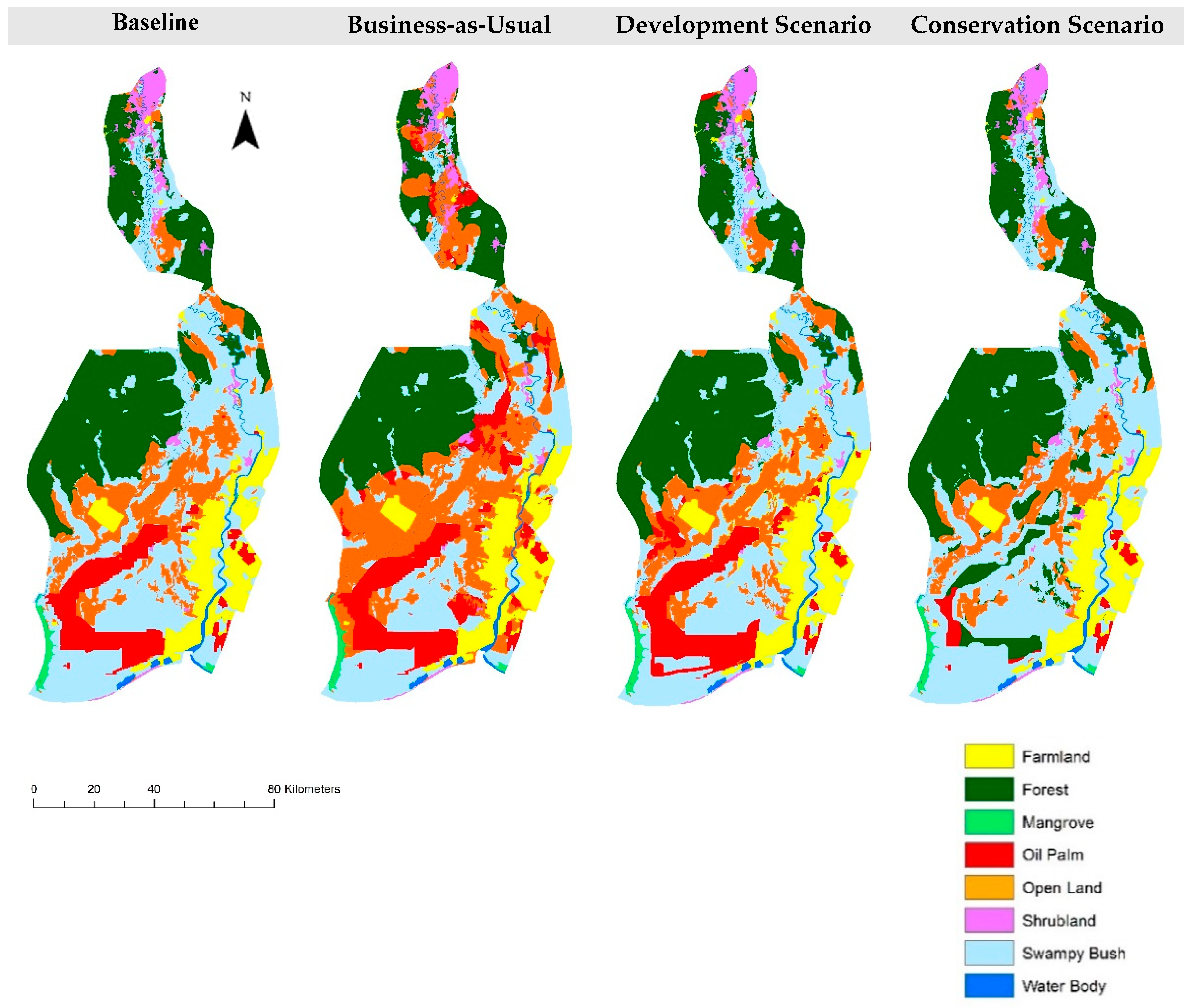
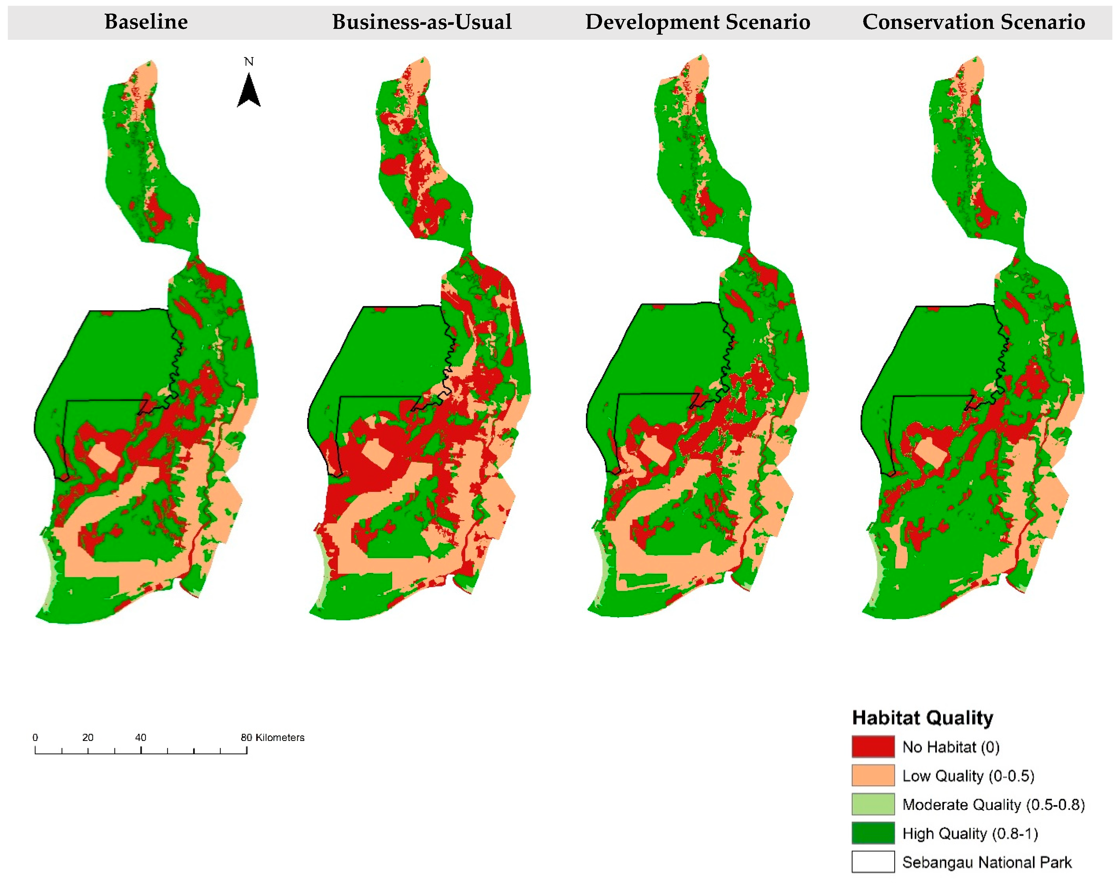
The authors modeled LULC changes and analyzed their effects on biodiversity under three different LULC scenarios. LCM and the InVEST Scenario Generator were used to model LULC, while the InVEST Habitat Quality tool was used to determine the effects on biodiversity. The study demonstrated that the trend of LULC change in the district will continue to be exacerbated in the BAU scenario, resulting in a higher loss of habitat quality for biodiversity. This loss is also well pronounced in the protected areas. Although agricultural expansion (development scenario) will result in lower habitat loss than the BAU scenario, there is a notable decrease in habitat quality due to external threats from surrounding anthropogenic land use practices. On the other hand, the LULC changes in the conservation scenario, which envision forest restoration, improve habitat quality for biodiversity. This shows that in terms of biodiversity, the regulated oil palm expansion in the DS is better off than BAU, where the oil palm expansion follows past trends. Also, if the government implements the restoration plan it will significantly improve habitat quality and biodiversity in the district. In summary, the continuing LULC changes will have a significant impact on the habitat quality and biodiversity in the district. This loss of biodiversity could be halted by implementing conservation measures such as the restoration of degraded lands.

The habitat quality modeling using scenarios in this study is comparable to other studies. [15,39,40,41]. Three scenarios were developed for a forested landscape in Iran, with business-as-usual, protection-based zoning, and collaborative zoning to map biodiversity changes to inform policymakers in the region [15]. The researchers held consultative meetings with conservation bodies in the region to develop scenarios that reflected changes in protected area boundaries in the landscape. Their results showed that excluding areas that are vulnerable to degradation from protection and establishing new protection in high quality forest cover resulted in an increase in high quality habitats in the landscape. In another study, the impact of land use change on biodiversity was assessed in five planned land reconfiguration futures, namely irrigated cropping, biodiversity and environmental planting, grazing, perennial horticulture, and agroforestry [41]. The investigators used the InVEST Habitat Quality model and demonstrated spatial approaches to classifying landscapes for habitat quality based on the size, density, and distribution of native vegetation in the landscape. A study in China modeled land use change and its effect on biodiversity conservation using two land use management scenarios [42]. The investigators developed scenarios based on the protection levels of the local government plans and projected biodiversity at local and regional scales.

We used an integrated modeling approach for scenario building, which is a distinguishable feature of this study. We modeled the LULC changes using statistical projection and vision-based scenario building processes. While the LCM used LULC from two points in time to project a future LULC based on the drivers of land cover change, the InVEST scenario generator simplified the process of modeling the future by using input from stakeholders and land suitability factors. However, there are several limitations to using the scenario-based approach for modeling biodiversity changes. First, although scenarios help to develop understanding of plausible future LULC, they are based on assumptions and do not represent an absolute future outcome. Second, the study considered LULC as a driving force of changes in biodiversity. However, many other important drivers influence biodiversity such as hunting, pollution and climate change, which are not captured in the model. In addition, other indirect factors, such as the market price of agricultural goods, which influence demand (and thus the need for an extension of plantations), were not incorporated in this study due to model limitations. As the models used in this study are not iterative and no validation was performed, there could be uncertainties regarding the results of this study. Therefore, where time and data are available, validation through field studies and more detailed finer resolution assessments would be suitable.

This study demonstrates a GIS-based integrated modeling approach to analyze the spatial pattern of LULC change under different scenarios and the resulting effects on habitat quality. Since the models can be used with readily available datasets, these methods could be used for rapid biodiversity assessments in data-poor regions like Indonesia. This study provides a real-world application of modeling to better inform land use planning and policies. The use of spatial tools to illustrate explicit LULC changes and their impact on habitat quality is useful in making land use management decisions. The conservation scenario in this study also provides a general guide to land managers and planners for the conservation of the pristine habitats in the district. Further, the approach of involving stakeholders contributes to sensitizing them to the impacts of LULC changes. During consultations, stakeholders were encouraged to develop appropriate land use management decisions for landscape-level conservation. The stakeholders also iterated that government persistence in biodiversity conservation and technical and financial support from the donor agencies is needed to implement the restoration plan. The findings of this study serve as a feasibility analysis based on a biophysical assessment of habitat quality. Further validation through review and in-depth field studies is recommended. Although biodiversity conservation results in improvements in many ESs there are several tradeoffs. Thus, it is essential to explore the synergies and tradeoffs between biodiversity and ecosystem services in landscape level planning. We recommend further studies on other important ecosystem services in the district to improve the findings of this study.

References

1. Butchart, S.H.; Walpole, M.; Collen, B.; Van Strien, A.; Scharlemann, J.P.; Almond, R.E.; Baillie, J.E.; Bomhard, B.; Brown, C.; Bruno, J. Global Biodiversity: Indicators of recent declines. Science 2010, 328, 1164–1168. [Google Scholar] [CrossRef] [PubMed]
2. MEA. Ecosystems and Human Well-Being: A Framework for Assessment; Island Press: Washington, DC, USA, 2005. [Google Scholar]
3. Tilman, D. Biodiversity: Population versus ecosystem stability. Ecology 1996, 77, 350–363. [Google Scholar] [CrossRef]
4. Chapin, F.S.; Zavaleta, E.S.; Eviner, V.T.; Naylor, R.L.; Vitousek, P.M.; Reynolds, H.L.; Hooper, D.U.; Lavorel, S.; Sala, O.E.; Hobbie, S.E. Consequences of changing biodiversity. Nature 2000, 405, 234–242. [Google Scholar] [CrossRef] [PubMed]
5. Díaz, S.; Fargione, J.; Chapin, F.S.; Tilman, D. Biodiversity loss threatens human well-being. PLoS Biol. 2006, 4, e277. [Google Scholar] [CrossRef] [PubMed]
6. Pimm, S.L.; Raven, P. Biodiversity: Extinction by numbers. Nature 2000, 403, 843–845. [Google Scholar] [CrossRef] [PubMed]
7. Newbold, T.; Hudson, L.N.; Hill, S.L.; Contu, S.; Lysenko, I.; Senior, R.A.; Börger, L.; Bennett, D.J.; Choimes, A.; Collen, B. Global effects of land use on local terrestrial biodiversity. Nature 2015, 520, 45–50. [Google Scholar] [CrossRef] [PubMed] [Green Version]
8. Sala, O.E.; Chapin, F.S.; Armesto, J.J.; Berlow, E.; Bloomfield, J.; Dirzo, R.; Huber-Sannwald, E.; Huenneke, L.F.; Jackson, R.B.; Kinzig, A. Global biodiversity scenarios for the year 2100. Science 2000, 287, 1770–1774. [Google Scholar] [CrossRef] [PubMed]
9. Schmitz, C.; van Meijl, H.; Kyle, P.; Nelson, G.C.; Fujimori, S.; Gurgel, A.; Havlik, P.; Heyhoe, E.; d’Croz, D.M.; Popp, A. Land-use change trajectories up to 2050: Insights from a global agro-economic model comparison. Agric. Econ. 2014, 45, 69–84. [Google Scholar] [CrossRef]
10. Iverson, L.; Echeverria, C.; Nahuelhual, L.; Luque, S. Ecosystem services in changing landscapes: An introduction. Landsc. Ecol. 2014, 29, 181–186. [Google Scholar] [CrossRef]
11. Secretariat of the Intergovernmental Science-Policy Platform on Biodiversity and Ecosystem Services (IPBES). The Methodological Assessment Report on Scenarios and Models of Biodiversity and Ecosystem Services; IPBES: Bonn, Germany, 2016; p. 348. [Google Scholar]
12. The Economics of Ecosystems and Biodiversity (TEEB). The Economics of Ecosystems and Biodiversity: Mainstreaming the Economics of Nature: A Synthesis of the Approach, Conclusions and Recommendations of TEEB; TEEB: Nagoya, Japan, 2010. [Google Scholar]
13. Polasky, S.; Carpenter, S.R.; Folke, C.; Keeler, B. Decision-making under great uncertainty: Environmental management in an era of global change. Trends Ecol. Evol. 2011, 26, 398–404. [Google Scholar] [CrossRef] [PubMed]
14. Baral, H.; Keenan, R.J.; Sharma, S.K.; Stork, N.E.; Kasel, S. Economic evaluation of ecosystem goods and services under different landscape management scenarios. Land Use Policy 2014, 39, 54–64. [Google Scholar] [CrossRef]
15. Zarandian, A.; Baral, H.; Stork, N.E.; Ling, M.A.; Yavari, A.R.; Jafari, H.R.; Amirnejad, H. Modeling of ecosystem services informs spatial planning in lands adjacent to the sarvelat and javaherdasht protected area in northern Iran. Land Use Policy 2017, 61, 487–500. [Google Scholar] [CrossRef]
16. Hamilton, C.M.; Martinuzzi, S.; Plantinga, A.J.; Radeloff, V.C.; Lewis, D.J.; Thogmartin, W.E.; Heglund, P.J.; Pidgeon, A.M. Current and future land use around a nationwide protected area network. PLoS ONE 2013, 8, e55737. [Google Scholar] [CrossRef] [PubMed] [Green Version]
17. Baral, H.; Keenan, R.J.; Stork, N.E.; Kasel, S. Measuring and managing ecosystem goods and services in changing landscapes: A south-east australian perspective. J. Environ. Plan. Manag. 2013, 57, 961–983. [Google Scholar] [CrossRef]
18. Baral, H.; Jaung, W.; Bhatta, L.D.; Phuntsho, S.; Sharma, S.; Paudyal, K.; Zarandian, A.; Sears, R.; Sharma, R.; Dorji, T. Approaches and Tools for Assessing Mountain Forest Ecosystem Services; CIFOR: Bogor, Indonesia, 2018; Volume 235. [Google Scholar]
19. Wilson, T.; Sleeter, B.; Sleeter, R.; Soulard, C. Land-use threats and protected areas: A scenario-based, landscape level approach. Land 2014, 3, 362–389. [Google Scholar] [CrossRef]
20. National Research Council. Advancing Land Change Modeling: Opportunities and Research Requirements; National Academies Press: Washington, DC, USA, 2014. [Google Scholar]
21. Atkinson, G.; Bateman, I.; Mourato, S. Recent advances in the valuation of ecosystem services and biodiversity. Oxford Rev. Econ. Policy 2012, 28, 22–47. [Google Scholar] [CrossRef]
22. Zlinszky, A.; Heilmeier, H.; Balzter, H.; Czúcz, B.; Pfeifer, N. Remote Sensing and GIS for Habitat Quality Monitoring: New Approaches and Future Research; Multidisciplinary Digital Publishing Institute: Basel, Switzerland, 2015.
23. Lengyel, S.; Déri, E.; Varga, Z.; Horváth, R.; Tóthmérész, B.; Henry, P.-Y.; Kobler, A.; Kutnar, L.; Babij, V.; Seliškar, A. Habitat monitoring in europe: A description of current practices. Biodivers. Conserv. 2008, 17, 3327–3339. [Google Scholar] [CrossRef]
24. Johnson, M.D.; Arcata, C. Habitat quality: A brief review for wildlife biologists. Trans. West. Sect. Wildl. Soc. 2005, 41, 31. [Google Scholar]
25. Olosutean, H. Methods for modeling ecosystem services: A review. Manag. Sustain. Dev. 2015, 7, 5–12. [Google Scholar] [CrossRef]
26. Johnson, M.D. Measuring habitat quality: A review. Condor 2007, 109, 489–504. [Google Scholar] [CrossRef]
27. Posa, M.R.C.; Wijedasa, L.S.; Corlett, R.T. Biodiversity and conservation of tropical peat swamp forests. BioScience 2011, 61, 49–57. [Google Scholar] [CrossRef]
28. Wilcove, D.S.; Koh, L.P. Addressing the threats to biodiversity from oil-palm agriculture. Biodivers. Conserv. 2010, 19, 999–1007. [Google Scholar] [CrossRef]
29. Broich, M.; Hansen, M.; Stolle, F.; Potapov, P.; Margono, B.A.; Adusei, B. Remotely sensed forest cover loss shows high spatial and temporal variation across Sumatra and Kalimantan, Indonesia 2000–2008. Environ. Res. Lett. 2011, 6, 014010. [Google Scholar] [CrossRef]
30. Koh, L.P.; Wilcove, D.S. Is oil palm agriculture really destroying tropical biodiversity? Conserv. Lett. 2008, 1, 60–64. [Google Scholar] [CrossRef]
31. BPS-Statistics of Pulang Pisau Regency. Kabupaten Pulang Pisau Dalam Angka (Pulang Pisau Regency in Figures); BPS-Statistics of Pulang Pisau Regency: Pulang Pisau, Indonesia, 2016.
32. Houterman, J.; Ritzema, H. Master Plan for the Rehabilitation and Revtalization of the Ex-Mega Rice Project Area in Central Kalimantan; Government of Indonesia and Royal Netherlands Embassy: Jakarta, Indonesia, 2009.
33. District Government of Pulang Pisau (DGPP). Green Growth Strategy: Pulang Pisau 2015; District Government of Pulang Pisau, Provincial Government of Central Kalimantan, Ministry of National Development Planning (BAPPENAS) and the Global Green Growth Institute (GGGI): Pulang Pisau, Indonesia, 2015.
34. Cheyne, S.M.; Thompson, C.J.; Phillips, A.C.; Hill, R.M.; Limin, S.H. Density and population estimate of gibbons (hylobates albibarbis) in the sabangau catchment, Central Kalimantan, Indonesia. Primates 2008, 49, 50–56. [Google Scholar] [CrossRef] [PubMed]
35. Morrogh-Bernard, H.; Husson, S.; Page, S.; Rieley, J. Population status of the bornean orang-utan (pongo pygmaeus) in the sebangau peat swamp forest, Central Kalimantan, Indonesia. Biol. Conserv. 2003, 110, 141–152. [Google Scholar] [CrossRef]
36. Eastman, J.; Van Fossen, M.; Solarzano, L. Transition potential modeling for land cover change. In GIS, Spatial Analysis and Modeling; ESRI Press: Redlands, CA, USA, 2005; pp. 357–386. [Google Scholar]
37. The Natural Capital Project. Invest User Guide: Scenario Generator. Available online: http://data.naturalcapitalproject.org/nightly-build/invest-users-guide/html/scenario_generator.html (accessed on 7 February 2018).
38. Sharp, R.; Tallis, H.T.; Ricketts, T.; Guerry, A.D.; Wood, S.A.; Chaplin-Kramer, R.; Nelson, E.; Ennaanay, D.; Wolny, S.; Olwero, N.; et al. Invest 3.4.0 User’s Guide; Stanford University, University of Minnesota, The Nature Conservancy, and World Wildlife Fund: Minneapolis, MN, USA, 2016. [Google Scholar]
39. Bhagabati, N.; Barano, T.; Conte, M.; Ennaanay, D.; Hadian, O.; McKenzie, E.; Olwero, N.; Rosenthal, A.; Suparmoko, S.A.; Shapiro, A. A Green Vision for Sumatra: Using Ecosystem Services Information to Make Recommendations for Sustainable Land Use Planning at the Province and District Level; The Natural Capital Project: Stanford, CA, USA, 2012. [Google Scholar]
40. Sharma, S.K.; Baral, H.; Pacheco, P.; Laumonier, Y. Assessing Impacts on Ecosystem Services under Various Plausible Oil Palm Expansion Scenarios in Central Kalimantan, Indonesia; Center for International Forestry Research (CIFOR): Bogor, Indonesia, 2017. [Google Scholar]
41. Baral, H.; Keenan, R.J.; Sharma, S.K.; Stork, N.E.; Kasel, S. Spatial assessment and mapping of biodiversity and conservation priorities in a heavily modified and fragmented production landscape in North-Central Victoria, Australia. Ecol. Indic. 2014, 36, 552–562. [Google Scholar] [CrossRef]
42. Liang, Y.; Liu, L. Simulating land-use change and its effect on biodiversity conservation in a watershed in Northwest China. Ecosyst. Health Sustain. 2017, 3, 1335933. [Google Scholar] [CrossRef]
43. Polasky, S.; Nelson, E.; Pennington, D.; Johnson, K.A. The impact of land-use change on ecosystem services, biodiversity and returns to landowners: A case study in the state of Minnesota. Environ. Resour. Econ. 2011, 48, 219–242. [Google Scholar] [CrossRef]
44. Kuhnert, P.M.; Martin, T.G.; Griffiths, S.P. A guide to eliciting and using expert knowledge in bayesian ecological models. Ecol. Lett. 2010, 13, 900–914. [Google Scholar] [CrossRef] [PubMed]
Figure 1. Map of the study area in Pulang Pisau district, in Central Kalimantan.
Land 07 00057 g001
Figure 2. Conceptual framework showing the overall process associated with this study.
Land 07 00057 g002
Figure 3. Land use and land cover (LULC) under different scenarios.
Land 07 00057 g003
Figure 4. Spatial distribution of habitat quality in Baseline, BAU, DS, and CS.
Land 07 00057 g004