Predicted Maps for Soil Organic Matter Evaluation: The Case of Abruzzo Region (Italy)


Council for Agricultural Research and Economics, Research Centre for Agriculture and Environment, Via della Navicella 2–4, 00184 Rome, Italy
*
Author to whom correspondence should be addressed.
Land 2020, 9(10), 349; https://0-doi-org.brum.beds.ac.uk/10.3390/land9100349
Submission received: 25 August 2020
/
Revised: 21 September 2020
/
Accepted: 22 September 2020
/
Published: 24 September 2020
(This article belongs to the Special Issue Soil Management for Sustainability)
Abstract
:Organic matter, an important component of healthy soils, may be used as an indicator in sustainability assessments. Managing soil carbon storage can foster agricultural productivity and environmental quality, reducing the severity and costs of natural phenomena. Thus, accurately estimating the spatial variability of soil organic matter (SOM) is crucial for sustainable soil management when planning agro-environmental measures at the regional level. SOM variability is very large in Italy, and soil organic carbon (SOC) surveys considering such variability are difficult and onerous. The study concerns the Abruzzo Region (about 10,800 km2), in Central Italy, where data from 1753 soil profiles were available, together with a Digital Elevation Model (DEM) and Landsat images. Some morphometric parameters and spectral indices with a significant degree of correlation with measured data were used as predictors for regression-kriging (RK) application. Estimated map of SOC stocks, and of SOM related to USDA (United States Department of Agriculture) texture—an additional indicator of soil quality—were produced with a satisfactory level of accuracy. Results showed that SOC stocks and SOM concentrations in relation to texture were lower in the hilly area along the shoreline, pointing out the need to improve soil management to guarantee agricultural land sustainability.
1. Introduction
One of the main challenges for the future is to maintain soil functions, but despite many efforts to promote more sustainable land management, soil degradation in the European Union (EU) is increasing [1], with a severe impact on food production and the supply of ecosystem services. Among the soil properties impacting soil quality, soil organic carbon (SOC)—and soil organic matter (SOM) derived from its determination—deserves special attention, representing a key indicator for evaluating soil quality [2], but also impacting the chemical and physical properties of the soil and its overall health. Properties affected by organic matter include soil structure, water holding capacity, diversity and activity of soil organisms, buffering capacity, and nutrient availability. SOM also regulates the efficiency of soil amendments, fertilizers, pesticides, and herbicides. According to the Food and Agriculture Organization of the United Nations (FAO) [3], one of the characteristics of sustainable soil management (SSM) is a stable or increasing storage of SOM, ideally close to the optimal level for the local environment, for all land uses. Thus, the most efficient way to improve soil quality is to stimulate better SOM management.
SOC is also an essential component of the global carbon cycle [4], representing one of the largest reservoirs of terrestrial carbon that may influence global warming [5,6]. The global carbon budget, and the CO2 emissions associated with its major components (i.e., atmosphere, ocean, fossil fuels, soil, and biosphere) is vital to support the environmental policy addressing climate change [7]. SOC sequestration, resulting from increased soil C inputs and/or reduced C losses [1,8,9], has been recognized as an important process to mitigate the rise of the atmospheric greenhouse gas (GHG) concentration. SSM measures such as increasing SOC stocks can thus mitigate the climate change, at least for several years after their adoption [10].
Soil carbon losses are related to changes in land use, soil management, and climate change issues. Across Europe, most soils have unbalanced SOC/SOM contents, resulting from non-conservative land management practices and land use. The consequence is an acceleration of SOM decomposition [11], and opposing this process is highly advisable to ensure sustainability in European arable soils [12].
The decrease of SOC/SOM is particularly relevant within the Mediterranean area, in consequence of the decreased soil fertility and the increased risk of soil erosion and desertification [13]. It was estimated that 74% of the territory in southern Europe has soils with less than 2% of organic carbon (i.e., 3.4% organic matter in the shallow layers) [14]). In Italy, SOC/SOM variability is very high due to the peculiar geological and geomorphological situation, and soil surveys taking into consideration a similar variability are difficult and onerous. In areas with Mediterranean climates, like central and southern Italy, SOC/SOM degradation is higher due to the coupled effect of high temperatures and low soil moisture, increasing the mineralization rate. Moreover, lower SOC/SOM accumulation often results from intensive and non-conservative agronomic practices (e.g., deep tillage), usually adopted in clayey soils of these areas to enhance soil structure, permeability, and aeration, and to assist crop growth, especially in hilly lands [15,16]. A similar soil management causes higher aeration, accelerating the SOC/SOM degradation rate, and the mixing with underlying horizons with lower SOC/SOM, diluting SOC/SOM in the arable layer. The soil is thus more exposed to wind and water erosion [17]. Therefore, ongoing interest in ensuring a sustainable use and management of European soil resources give rise to a priority need for reliable quantitative information on the present state of SOC/SOM.
SOC/SOM distribution is controlled by many factors (e.g., climate, hydrology, soil type, land use, etc. [18]), whose spatial variation is often wide and not linear. Thus, an accurate estimate of such spatial variability is crucial in soil quality evaluation and in assessing the carbon sequestration potential, providing an operative tool for land use planners and decision makers. Mapping SOM is a common task in site-specific crop management, whereas mapping SOC and its changes over time is an important issue in research and in quantifying and monitoring changes in soil carbon stocks. Both objectives can be achieved at minimum cost and high accuracy and precision [19].
Up-to-date and accurate information on SOC/SOM is essential for tailoring site-specific management, but traditional mapping is labor-intensive, time-consuming, and requires expensive sample collection. Point samples at the local scale are usually more easily available, but such soil information needs to be interpolated in space from a limited number of observations, estimating soil properties over the whole area of interest. Studies have revealed that there is a significant correlation among terrain variables and SOC/SOM [20,21], meaning that spatial estimates can be improved by using auxiliary data—exhaustive and spatially extensive—that can provide relevant information at unsampled locations. It has been largely demonstrated that spatial prediction methods based on ancillary information usually produce maps with higher accuracy, given that the primary and secondary variables are significantly correlated [22,23]. Digital soil mapping (DSM) techniques have gained more increasing appeal in recent years, providing rapid and cost-efficient tools for mapping soil properties across large areas. These methods integrate measured data and auxiliary information, usually available at finer spatial resolution than the point values of a primary target sampled variable [24]. Several authors have used DSM techniques for SOC/SOM mapping, for example, Adhikari et al. [25] adopted regression-kriging (RK) in Denmark, using 18 environmental variables as predictors for mapping the spatial distribution of SOC. Guo et al. [26] applied random forest plus residuals kriging in an area of China to estimate the spatial arrangement of SOM. Song et al. [27] combined estimation methods with local terrain features to enhance their SOC prediction performance. Wang et al. [28] tested three machine learning techniques for mapping SOC stocks in Australia, using several environmental covariates from remote sensing. Lamichhane et al. [29] reviewed the applications of different DSM techniques reported in the scientific literature from 2013 until 2019 for mapping SOC concentration and stocks.
Spatial interpolation by RK is a method that merges a regression of the primary dependent variable on secondary ancillary variables with simple kriging of the regression residuals [30,31,32,33]. Ancillary information is often derived from the digital elevation model (DEM), which provides topographic information that allows for the calculation of terrain parameters, and from satellite imagery, both easily available at relatively low cost. Since maintaining or increasing SOM is one of the main targets of SSM, our research question was whether such a technique, already tested in limited areas in Italy [15,34], could be suitable for SOM assessment at the regional level. We hypothesized that RK could yield accurate estimates for site-specific analyses without further sampling expenses. The Abruzzo region in central Italy was chosen as the study area due to the complexity of its territory, and for the availability of suitable data for RK application.
In this framework, the study aimed to provide a spatial evaluation—at a regional level—of SOC, soil USDA (United States Department of Agriculture) texture, and SOM levels based on the soil texture from point data, estimating values in non-sampled locations by applying RK. Then, by transferring them into a GIS software, we can produce a reliable estimate and a valid evaluation tool for a SSM.
2. Materials and Methods
2.1. Study Area
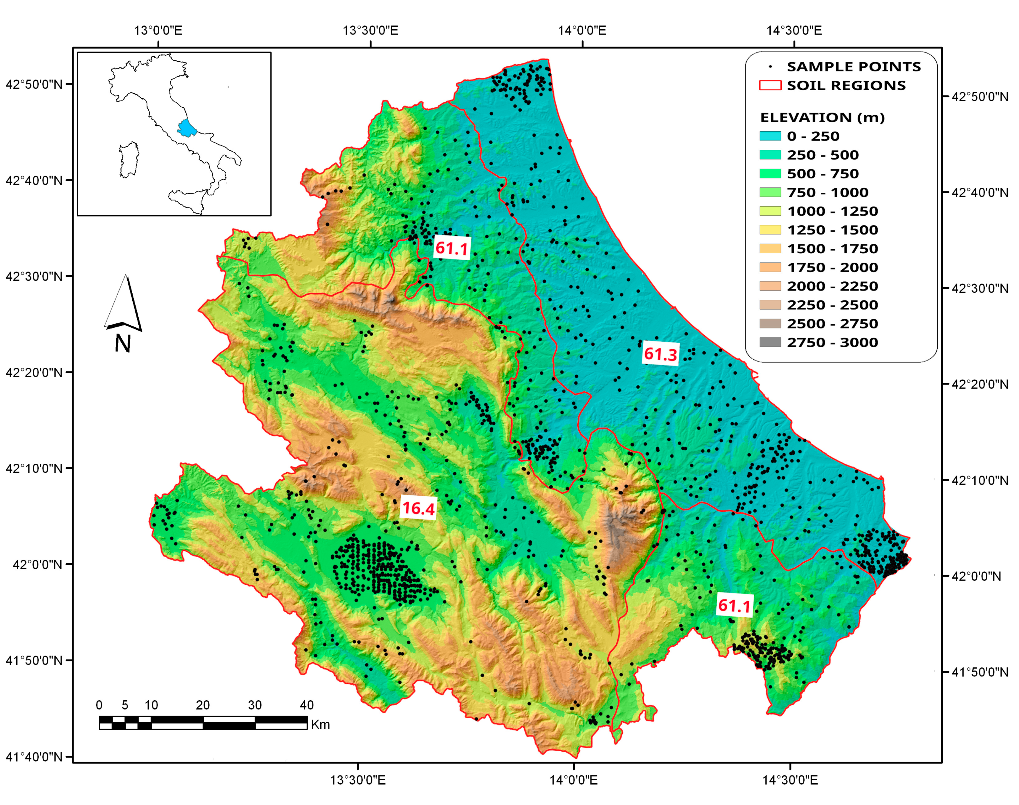
The study area, located in central Italy, consists of about 10,800 km2 corresponding to the territory of the Abruzzo region. Among the 20 administrative regions of Italy, Abruzzo is one of the most mountainous, located in the central peninsular part of the country. Bordered by the Adriatic Sea in the east and by the Apennines in the west, its territory is very complex and heterogeneous. Within a few kilometers, the environment changes from high mountains (Gran Sasso and Maiella) to the seashore, passing through all the intermediate landscapes: mountain grasslands and woods, hills, plains and river basins. While the mountain ranges lie along a NW–SE direction, the rivers cross them toward the sea along a SE–NW direction. About 40% of the total surface is represented by utilized agricultural area. Along the coastline, the climate is Mediterranean, warm and dry, gradually becoming continental moving inlands. Mean annual air temperature goes from 6 °C in the mountains to 15 °C near the sea. Mean annual rainfall ranges from 600–800 mm in the plains and in the river basins to 1000–1200 mm in the hills, reaching 1600 mm in the mountains. Summer is everywhere the dry season.
Soil regions (SR) are the largest units of soil description, depicting areas with similar soil-forming conditions. These are usually defined as typical associations of dominant soils, occurring in areas limited by a specific climate and/or a characteristic association of parent material. In our study area, soils belong to SRs 61.3, 61.1, and 16.4, as defined by the European Soil Bureau [35]:
- SR61.3: Hills of central and southern Italy on Pliocene and Pleistocene marine deposits and Holocene alluvial sediments along the Adriatic Sea;
- SR 61.1: Apennine and anti-Apennine relieves on sedimentary rocks (Tertiary arenaceous marly flysch) of central and southern Italy; and
- SR16.4: Apennine relieves on Mesozoic and Tertiary limestone, dolomite, and marl, and intra-mountain plains [36].
In Figure 1, the digital elevation model of the region is reported, together with the location of the sampling points and the boundaries of the SRs.
A land use map of the Abruzzo Region is reported as Supplementary Material (Figure S1).
2.2. Data Collection
The study dataset, provided by the Regional Agency for Agricultural Extension Services of Abruzzo Region (ARSSA), consists of 1753 georeferenced soil samples collected by an auger (0–25 and 25–50 cm) in accessible agricultural and forest land. The physical and chemical routine analyses included the measurement of particle size distribution according to the pipette method [37] and of SOC content according to the modified Walkley–Black method [38]. The SOC stock in kg m−2 for each soil profile was calculated as follows:
where soc is the organic carbon concentration in % for each soil horizon; bd is the bulk density of the soil horizon in g cm−3 estimated by suitable pedofunctions, different for each type of horizon [39]; th is the thickness of the horizon in cm; gr is the gravel content in %; and n is the number of horizons in the soil profile.
The SOM content was then evaluated from SOC [40] by means of the following formula:
SOM = SOC × 1.724
From an agronomic standpoint, the pedo-climatic context cannot be neglected in the evaluation of SOM, because in different soil types, the same amount of SOM can differently impact soil functions. Thus, the SOM content of the study area was classified into four different levels (i.e., very low, low, medium, and high) based on the USDA textural classes [41], as detailed in Table 1.
Land use, vegetation, climate, and terrain features are the main factors affecting soil properties at the landscape scale, particularly in hills, hence DEM-derived terrain attributes can be used for the prediction of the spatial distribution of soil features. Ancillary data for the area were derived from: (i) a 30 m degraded version of the 20 m DEM provided by the Land Information Service of the Abruzzo Region; (ii) from Landsat 7 TM imagery (three visible bands and four infrared bands), and (iii) the 1:250,000 Soil Subsystems Map of Abruzzo available from ARSSA [42].
From the DEM, the following morphometric attributes were derived:
- Elevation (ELEV);
- slope gradient (SLOPE);
- curvature plan and profile (PLANC and PROFC), obtained from the second derivative of the maximum slope direction and the perpendicular one respectively [43];
- solar radiation (SOLAR);
- Topographic Wetness Index (TWI);
- flow accumulation (FLOWACC), which represents the contributing area (i.e., the surface over which water from rainfall, snowfall, etc. can be aggregated) [44]; and
- Stream Power Index (SPI).
TWI is a parameter correlating topography and the water movement in slopes, used to display the spatial distribution of soil moisture and the shallow saturation degree:
where As is the specific catchment area and β is the slope [45].
TWI = ln(As/tanβ)
SPI is used to describe potential flow erosion and related landscape processes. When specific catchment area and slope steepness increase, both the amount of water contributed by upslope areas and the velocity of water flow also increase, hence stream power and potential erosion increase:
where As is the specific catchment area and β is the slope [46].
SPI = As × tanβ
From the Landsat 7 TM imagery (July 2016, cloud cover 0%), Clay Index (CI) and Normalized Difference Vegetation Index (NDVI) were calculated. CI is correlated with the clay content of the soil:
where MIR is Mid Infra Red (band 6) and MIR2 is Mid Infra Red (band 7) [47]. NDVI gives a quantitative and qualitative estimation of the vegetation:
where NIR is Near Infra Red (band 5) and R is Red (band 4) [48].
CI = MIR/MIR2
NDVI = (NIR − R)/(NIR + R)
From the 1:250,000 Soil Subsystems Map of Abruzzo Region by ARSSA [42], an additional variable—SST86—was derived, defined by 29 different soil systems and 87 soil subsystems. Converting the map into a raster, all these soil units were grouped in a single categorical variable.
Finally, a multivariate correlation analysis allowed us to consider as suitable covariates for prediction only those auxiliary data with a relatively stronger spatial correlation with the target soil variables.
2.3. Data Processing and Validation of Results
RK, a sort of BLUP (Best Linear Unbiased Prediction) method for spatial data, assumes that the local mean varies continuously into each neighborhood, and can be estimated by combining both directly measured data and correlated ancillary information [28,29]. The technique uses multiple regression to depict the relationship linking the field primary variable and the secondary data. Kriging is then applied to the regression residuals, and the results from both regression and kriging are joined to obtain the estimation [49,50].
The available measured dataset was randomly divided in a training dataset (75% of total samples), and a test dataset (25% of total samples), using only the training part for prediction and the test one to validate the results.
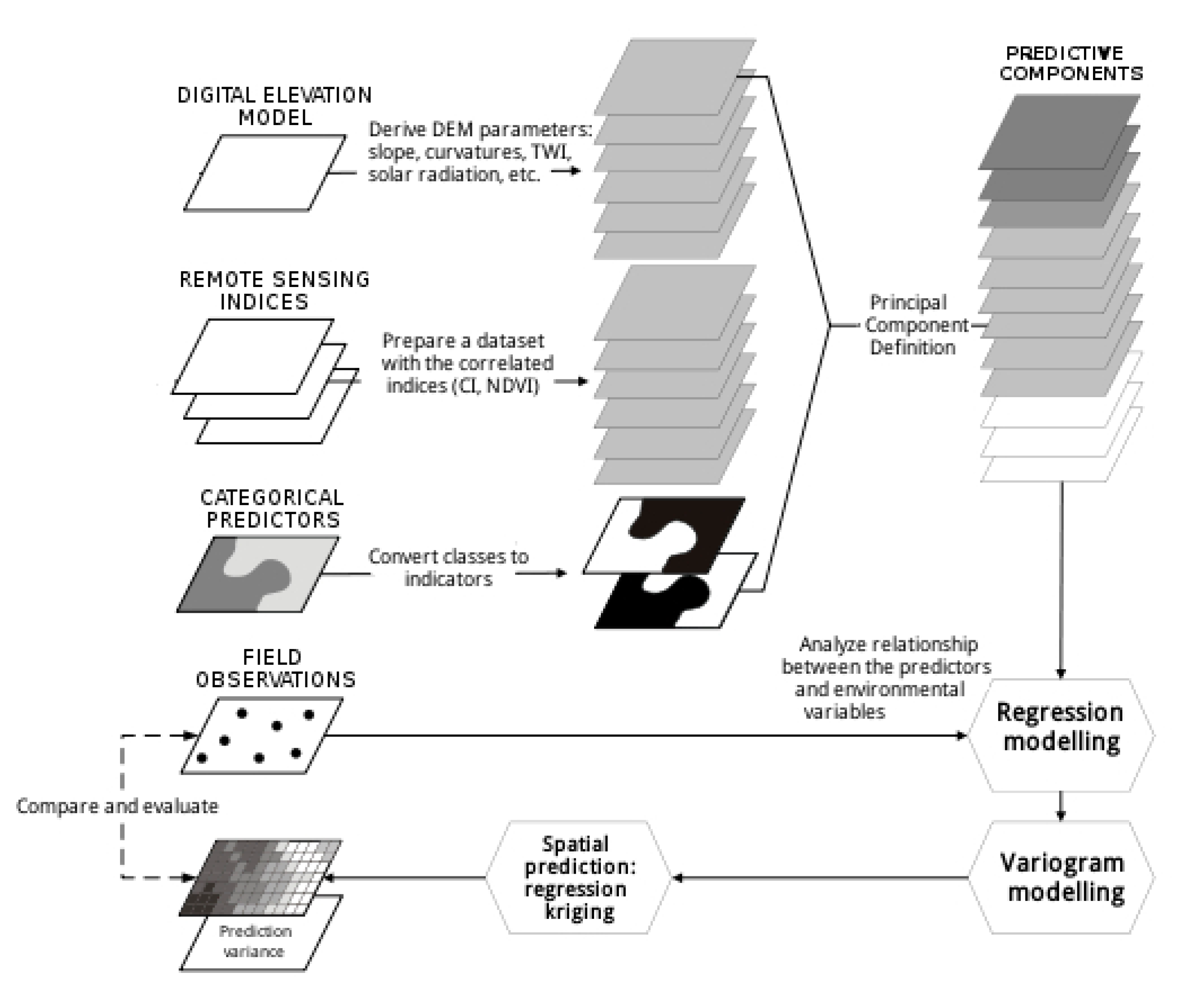
For estimating the target variables (SOC, sand and clay) by RK, the computational steps reported below were followed [34]:
- set up and import predictor data layers (land-surface parameters and soil subsystems map);
- match soil samples in the training dataset with land-surface parameters and build the regression matrix. Since using the calculated parameters and indices directly as predictors may cause multicollinearity and redundancy effects, the covariates were transformed in principal components (PCs) [51]. Eleven orthogonal and independent components were defined, and the choice of predictors for each variable was then performed by a stepwise regression, considering only the components significant at p < 0.001;
- linear regression analysis and derivation of the regression residuals, resolving the regression coefficients by means of a maximum likelihood algorithm [52];
- analysis of residuals for detecting spatial autocorrelation, and fitting of the theoretical variogram models;
- run the interpolation; and
- visualization and validation of the results using the test dataset.
A flowchart of the procedure is reported in Figure 2. The software SAGA 7.6.3 [53] and ILWIS 3.8.6 Open [54] were used for the derivation of parameters and indices, and for PCs definition. The statistical software R 3.6.3, with the packages sp and rgdal for spatial data preparation and gstat for geostatistical modeling and prediction, was used to perform the regression analysis [55]. The software ArcGIS 10.2® was used for drawing the estimated maps of SOC in kg m−2, soil texture (USDA classification), and SOM levels based on the USDA texture as specified in Table 1.
To assess the precision of prediction, estimated values from the training dataset were compared with the correspondent values from the test dataset and not used in the estimation procedure. Such validation allowed us to evaluate the accuracy of the prediction model by measuring the root mean square prediction error (RMSE):
where (xi) and Z(xi) are the estimated values and actual observations, respectively, and N is the number of validation points. The RMSE expresses the difference between the model estimations and the observed values, presented in the same unit of measurement. If the value of RMSE is close (lower) to the standard deviation of the data, then the model is a good fit [56]. The Geostatistical Analyst extension of the software ArcGIS 10.2® was used to validate the estimation results.
3. Results and Discussion
Pre-processing of data included basic statistics calculation and frequency distribution analysis. Two variables needed to be transformed to approach a normal distribution: sand (square root) and SOC (cube root). The 11 parameters and indices derived from ancillary data (ELEVATION, SLOPE, PROFC, PLANC, TWI, SOLAR, FLOWACC, SPI, CI, NDVI, SST86) were converted in PCs. Table 2 shows the matrix of transformation coefficients, calculated from the covariance matrix. The PC1 and PC2 components were the most significant ones for the prediction of all the target variables. The last component—PC11—was excluded a priori to avoid any rounding effect in the PCs computation with ILWIS [46].
The target variables were strongly correlated with the principal components, as can be seen from the R2 values from the linear regression. As explained in the previous section, the choice of the components to be used as predictors was performed by the stepwise regression, considering a significance level of 0.001. For SOC estimation, the sum of PC1—PC2—PC3—PC5—PC7 was used; for sand estimation, the predictor was the sum of PC1—PC2—PC5—PC6—PC10 components; for clay estimation, the sum of PC1—PC2—PC3—PC4—PC6—PC10 components was chosen. Notably, all the components selected as predictors were related to the soil type and position.
RK was applied to the SOC content of the training dataset as well as to the sand and clay data to estimate soil texture. The prediction accuracy was evaluated comparing the values estimated using the training dataset with the measured values from the test dataset that did not enter in the estimation. The calculated RMSE was 0.31 for SOC, 1.76 for sand, and 11.56 for clay, lower than the standard deviation of the measured data of 0.38, 2.09, and 15.02, respectively, and thus considered a very good result, notwithstanding the irregular distribution of the sampling points.
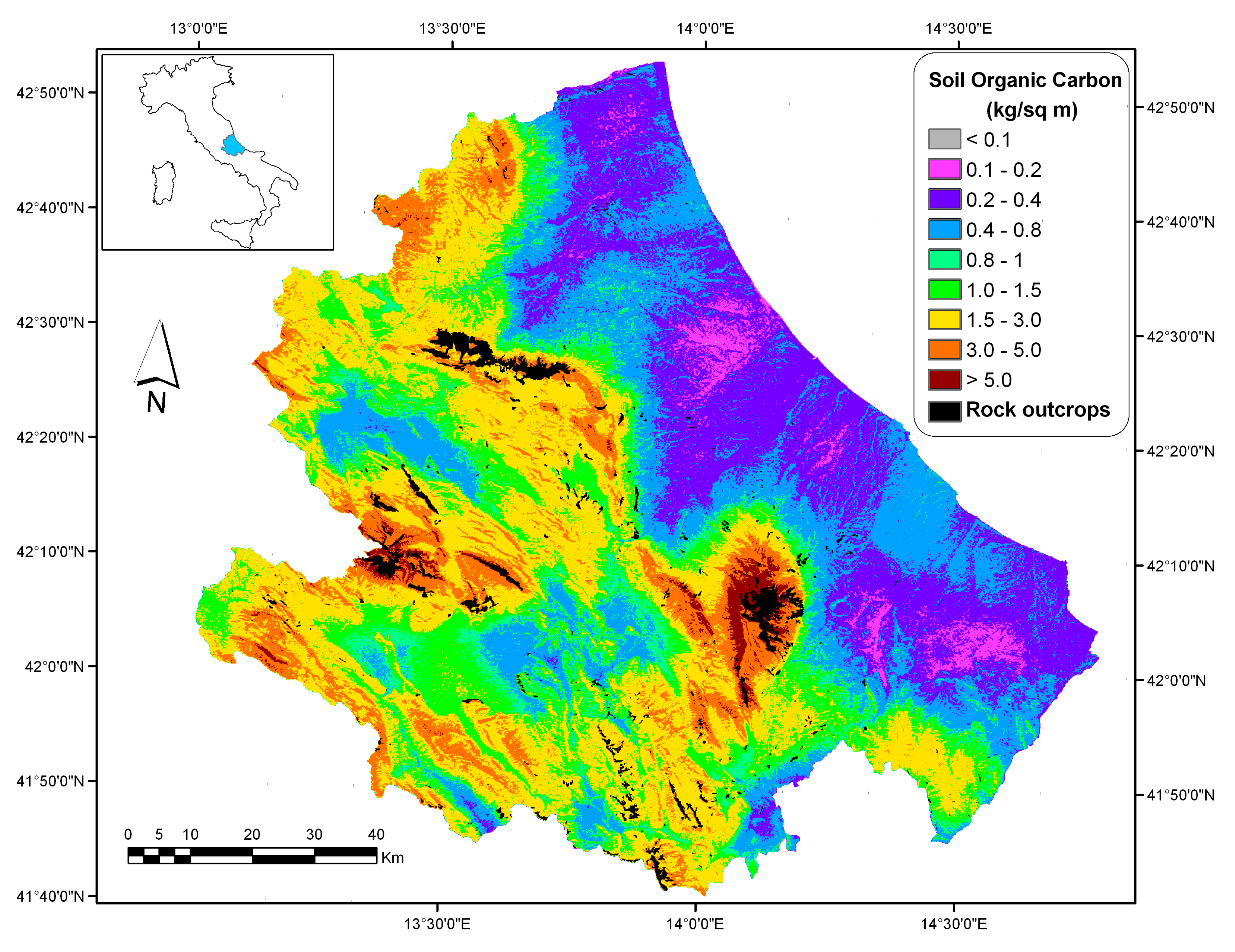
In Figure 3, the estimated map of SOC is reported, showing that about 88% of the area has a SOC content below 3.0 kg m−2.
In Figure 4, the map of USDA soil texture, estimated from sand and clay data using the training dataset, is reported, showing that the prevailing textures are loam and sandy loam.
Finally, SOM in g kg−1 was evaluated from SOC (Equation (2)), then SOM values were ranked in four classes (very low, low, medium, high) based on the estimated USDA texture (according to Table 1). The obtained map is reported in Figure 5.
The observed SOM levels were related to soil morphology: in the hilly belt along the coast, the map shows essentially a very low content, while in the interior, where soils are mainly under forest, the SOM content reached a high class in most of the territory (about 53%). In the coastal area, the SOM depletion can be considered both as a cause and effect of the active erosion on hills, usually exacerbated by intensive agricultural practices. This area is indeed intensely cropped, as can be seen from the land use map (Figure S1). Previous studies of the same type carried out in the northern part of the region, concerning a vineyard district, showed that an intervention to enhance SOM content is necessary [15,16,23,34]. Such a result is in line with the findings by Berhongaray et al. [57], who reported that cultivation caused a reduction of 16% in SOC content at 50 cm depth in the Argentine Pampas.
In Abruzzo, an improvement in agro-environmental planning is required to ensure an appropriate SOC/SOM content to soils, so that they can maintain their ecological and socio-economical functions, and crop yield sustainability in agricultural lands. Stimulating the adoption of SSM practices through the dissemination activity of agricultural extension services is fundamental to preserve soil resources. Such practices can enhance soil quality (water holding capacity, infiltration, soil structure, and soil fertility), improve the SOM cycle, and effectively contribute to climate change mitigation. A rational soil management can also help to reduce GHG emissions, especially carbon dioxide emissions, favoring a decrease in soil organic carbon losses, increasing the organic matter input, or combining both of them [15].
This study, defining the current SOC/SOM status in a region of central Italy, provides evidence that SOM management in its agricultural areas should be improved. The results of our study show that in Abruzzo, most arable lands are susceptible to soil degradation, sped-up by dry conditions and high temperatures causing a rapid mineralization of SOM. These areas need appropriate management to guarantee agricultural land sustainability. Adopting conservative practices such as conservation tillage or no-tillage (e.g., direct seeding), improving rotations with forage crops, returning crop residues to soil, growing green manure crops, and supplying the soil with proper exogenous organic matter could lead to an appropriate SOM restoration [16]. Permanent grasslands are effective for soil carbon accumulation in mineral soils and the adoption of agroforestry—the integration of trees and shrubs on agricultural land—and crop diversification might contribute to SSM [1].
An accurate state-of-the-art of SOC/SOM distribution would allow us to foresee future trends, and to evaluate the effectiveness of soil conservation practices stabilizing and increasing carbon stock in soils, which should be adopted for a more sustainable soil management. As in our case, mapping SOC over a large area in Bosnia and Herzegovina by classical geostatistical methods [58] showed that the spatial distribution of SOC concentration was strongly influenced by the intense farming practices. In this case, however, the environmental variables had a reduced capacity to explain the spatial variability of SOC. In Brazil, Bonfatti et al. [59] applied RK for mapping SOC, finding again a similar situation: soils under arable crops and vineyard showed the lowest concentration.
In the northern part of Abruzzo, similar mapping work was carried out comparing ordinary kriging and RK as spatial interpolators, and their performance resulted in being approximately the same [34], depending on the available auxiliary information. Mapping targeted soil parameters such as SOC/SOM applying RK, both in limited areas [15] and at the regional level, can represent a valid tool, providing useful and accurate information to assess soil degradation in a cost-effective and little time-consuming way. Such maps can also improve the process of carbon budgeting and reporting—in line with global initiatives of minimizing greenhouse gas emission—and thus the impacts of climate change [60]. Moreover, they can really help farmers in managing soils, can influence and support local land-use planners, and can also be easily updated whenever new data become available.
4. Conclusions
A spatial representation of SOM is essential to supply a useful and proper reference tool to decision makers, facilitating and optimizing the regional planning of agro-environmental measures for a SSM. Soil surveys taking into account the extremely large variability of the Italian territory are very difficult and onerous. However, most soil attributes are spatially correlated with ancillary variables derived from DEM, Landsat imagery. and existing soil subsystem maps.
In the Abruzzo region, analyzing the available data and estimating values in non-sampled locations by means of RK—integrating measured data and ancillary variables—allowed us to map soil texture, SOC, and SOM levels based on the USDA texture with an acceptable precision. These maps, obtained at relatively low costs, could also be less accurate than the traditional ones, but providing the associated estimation error may anyway bring added value. The observed SOC/SOM distribution appears to be linked to the soil morphology and to the land use: low or very low in intensively cropped hills near the shore, and high in mountains and forest land.
RK proved to be a rapid and cost-efficient tool for mapping soil properties across large areas, allowing us to easily monitor their changes over time. Maps can be updated every time new information and/or new data become available. In the next future, it is hoped that this technique will be successfully coupled and associated with traditional soil surveying and mapping procedures, and then applied at the national level.
Supplementary Materials
The following are available online at https://0-www-mdpi-com.brum.beds.ac.uk/2073-445X/9/10/349/s1, Figure S1: Land use map (from CORINE Land Cover, https://land.copernicus.eu/pan-european/corine-land-cover/clc2018).
Author Contributions
Conceptualization, C.P., R.F., and A.M.; Investigation, C.P., R.F., and A.M.; Methodology, C.P., R.F. and A.M.; Validation, C.P., R.F. and A.M.; Writing—original draft, C.P.; Writing—review & editing, R.F. and A.M. All authors have read and agreed to the published version of the manuscript.
Funding
This research received no external funding.
Acknowledgments
The authors wish to thank Sergio Santucci and Igino Chiuchiarelli from ARRSA—Agricultural Extension Service of Abruzzo Region—for providing the soil dataset.
Conflicts of Interest
The authors declare no conflict of interest.
References
- Hagemann, N.; Álvaro-Fuentes, J.; Siebielec, G.; Castañeda, C.; Bartke, S.; Dietze, V.; Maring, L.; Arrúe, J.L.; Playán, E.; Plaza-Bonilla, D.; et al. Review of Economic, Social and Environmental Impacts and Implementation Barriers for Soil Protection and Sustainable Management Measures for Arable Land across the EU; European Commission, DG Environment, Technical Report, 2019; Contract no. ENV.D.1/SER/2016/0041; European Commission: Luxembourg, 2016. [Google Scholar]
- Gregorich, E.G.; Carter, M.R.; Angers, D.A.; Monreal, C.M.; Ellert, B.H. Toward minimum data set to assess soil organic matter quality in agricultural soils. Can. J. Soil Sci. 1994, 74, 885–901. [Google Scholar] [CrossRef] [Green Version]
- Food and Agriculture Organization of the United Nations. FAO Voluntary Guidelines for Sustainable Soil Management; FAO: Rome, Italy, 2017; p. 16. Available online: http://www.fao.org/3/a-bl813e.pdf (accessed on 18 August 2020).
- Smith, P.; Fang, C.M.; Dawson, J.J.C.; Moncrieff, J.B. Impact of global warming on soil organic carbon. Adv. Agron. 2008, 97, 1–43. [Google Scholar]
- Lützow, M.V.; Kögel-Knabner, I.; Ekschmitt, K.; Matzner, E.; Guggenberger, G.; Marschner, B.; Flessa, H. Stabilization of soil organic matter in temperate soils: Mechanisms and their relevance under different soil conditions—A review. Eur. J. Soil Sci. 2006, 57, 426–445. [Google Scholar] [CrossRef]
- Batjes, N.H. Total carbon and nitrogen in the soils of the world. Eur. J. Soil Sci. 1996, 47, 151–163. [Google Scholar] [CrossRef]
- Friedlingstein, P.; Jones, M.W.; O’Sullivan, M.; Andrew, R.M.; Hauck, J.; Peters, G.P.; Peters, W.; Pongratz, J.; Sitch, S.; Le Quéré, C.; et al. Global Carbon Budget 2019. Earth Syst. Sci. Data 2019, 11, 1783–1838. [Google Scholar] [CrossRef] [Green Version]
- Freibauer, A.; Rounsevell, M.D.A.; Smith, P.; Verhagen, J. Carbon sequestration in the agricultural soils of Europe. Geoderma 2004, 122, 1–23. [Google Scholar] [CrossRef]
- Baker, J.M.; Ochsner, T.E.; Venterea, R.T.; Griffis, T.J. Tillage and soil carbon sequestration—What do we really know? Agric. Ecosyst. Environ. 2007, 118, 1–5. [Google Scholar] [CrossRef]
- Lal, R. Soil carbon sequestration to mitigate climate change. Geoderma 2004, 123, 1–22. [Google Scholar] [CrossRef]
- Smith, P.; Andren, O.; Karlsson, T.; Perala, P.; Regina, K.; Rounsevell, M.; Van Wesemael, B. Carbon sequestration potential in European croplands has been overestimated. Glob. Chang. Biol. 2005, 11, 2153–2163. [Google Scholar] [CrossRef]
- Lal, R. Challenges and opportunities in soil organic matter research. Eur. J. Soil Sci. 2009, 60, 158–169. [Google Scholar] [CrossRef]
- Francaviglia, R.; Renzi, G.; Rivieccio, R.; Marchetti, A.; Piccini, C. Spatial analysis and prediction of soil organic carbon in Friuli Venezia Giulia Region (Northern Italy). Geoinfor. Geostat. Overv. 2014, 2. [Google Scholar] [CrossRef]
- Zdruli, P.; Jones, R.J.A.; Montanarella, L. Organic Matter in the Soils of Southern Europe. European Soil Bureau Technical Report; EUR 21083 EN; Office for Official Publications of the European Communities: Luxembourg, 2004. [Google Scholar]
- Marchetti, A.; Piccini, C.; Francaviglia, R.; Santucci, S.; Chiuchiarelli, I. Estimating soil organic matter content by regression kriging. In Digital Soil Mapping: Bridging Research, Environmental Application, and Operation; Boettinger, J.L., Howell, D.W., Moore, A.C., Hartemink, A.E., Kienast Brown, S., Eds.; Springer: Dordrecht, The Netherlands, 2010; pp. 241–254. [Google Scholar]
- Marchetti, A.; Piccini, C.; Francaviglia, R.; Mabit, L. Spatial distribution of soil organic matter using geostatistics: A key indicator to assess soil degradation status in central Italy. Pedosphere 2012, 22, 230–242. [Google Scholar] [CrossRef]
- Bot, A.; Benites, J. The Importance of Soil Organic Matter. Key to Drought-Resistant Soil and Sustained Food Production; FAO Soil Bulletin: Rome, Italy, 2005; Available online: http://www.fao.org/docrep/009/a0100e/a0100e00.htm (accessed on 18 August 2020).
- Fang, X.; Xue, Z.; Li, B.; An, S. Soil organic carbon distribution in relation to land use and its storage in a small watershed of the Loess Plateau, China. Catena 2012, 88, 6–13. [Google Scholar] [CrossRef]
- Ping, J.L.; Dobermann, A. Variation in the precision of soil organic carbon maps due to different laboratory and spatial prediction methods. Soil Sci. 2006, 171, 374–387. [Google Scholar]
- Mueller, T.G.; Pierce, F.J. Soil carbon maps: Enhancing spatial estimates with simple terrain attributes at multiple scales. Soil Sci. Soc. Am. J. 2003, 67, 258–267. [Google Scholar] [CrossRef]
- Dobos, E.; Carré, F.; Hengl, T.; Reuter, H.I.; Tóth, G. Digital Soil Mapping As a Support to Production of Functional Maps; EUR 22123 EN; Office for Official Publications of the European Communities: Luxemburg, 2006. [Google Scholar]
- McBratney, A.B.; Mendonça Santos, M.L.; Minasny, B. On digital soil mapping. Geoderma 2003, 117, 3–52. [Google Scholar] [CrossRef]
- Marchetti, A.; Piccini, C.; Francaviglia, R.; Santucci, S.; Chiuchiarelli, I. Evaluation of soil organic matter content in Teramo province, Central Italy. Adv. GeoEcol. 2008, 39, 345–356. [Google Scholar]
- McBratney, A.; Odeh, I.; Bishop, T.; Dunbar, M.; Shatar, T. An overview of pedometric techniques for use in soil survey. Geoderma 2000, 97, 293–327. [Google Scholar] [CrossRef]
- Adhikari, K.; Hartemink, A.E.; Minasny, B.; Bou Kheir, R.; Greve, M.B.; Greve, M.H. Digital Mapping of Soil Organic Carbon Contents and Stocks in Denmark. PLoS ONE 2014, 9, e105519. [Google Scholar] [CrossRef]
- Guo, P.T.; Li, M.F.; Luo, W.; Tang, Q.F.; Liu, Z.W.; Lin, Z.M. Digital mapping of soil organic matter for rubber plantation at regional scale: An application of random forest plus residuals kriging approach. Geoderma 2015, 237–238, 49–59. [Google Scholar] [CrossRef]
- Song, X.; Liu, F.; Zhang, G.; Li, D.; Zhao, Y.; Yang, J. Mapping soil organic carbon using local terrain attributes: A comparison of different polynomial models. Pedosphere 2017, 27, 681–693. [Google Scholar] [CrossRef]
- Wang, B.; Waters, C.; Orgill, S.; Gray, J.; Cowie, A.; Clark, A.; Liu, D.L. High resolution mapping of soil organic carbon stocks using remote sensing variables in the semi-arid rangelands of eastern Australia. Sci. Total Environ. 2018, 630, 367–378. [Google Scholar] [CrossRef] [PubMed]
- Lamichhane, S.; Kumar, L.; Wilson, B. Digital soil mapping algorithms and covariates for soil organic carbon mapping and their implications: A review. Geoderma 2019, 352, 395–413. [Google Scholar] [CrossRef]
- Odeh, I.O.A.; McBratney, A.B.; Chittleborough, D.J. Spatial prediction of soil properties from landform attributes derived from a digital elevation model. Geoderma 1994, 63, 197–214. [Google Scholar] [CrossRef]
- Goovaerts, P. Geostatistics for Natural Resource Evaluation; Oxford University Press: New York, NY, USA, 1997. [Google Scholar]
- Hengl, T.; Heuvelink, G.B.M.; Rossiter, D.G. About regression kriging: From equations to case studies. Comput. Geosci. 2007, 33, 1301–1315. [Google Scholar] [CrossRef]
- Sun, W.; Minasny, B.; McBratney, A. Analysis and prediction of soil properties using local regression-kriging. Geoderma 2012, 171–172, 16–23. [Google Scholar] [CrossRef]
- Piccini, C.; Marchetti, A.; Francaviglia, R. Estimation of soil organic matter by geostatistical methods: Use of auxiliary information in agricultural and environmental assessment. Ecol. Indic. 2014, 36, 301–314. [Google Scholar] [CrossRef]
- European Communities. European Soil Bureau Georeferenced Soil Database for Europe: Manual of Procedures, Version 1.1; EUR 18092 EN; Office for Official Publications of the European Communities: Luxemburg, 2001; p. 178. [Google Scholar]
- Costantini, E.A.C.; Urbano, F.; L’Abate, G. Soil Regions of Italy. 2004. Available online: http://www.soilmaps.it (accessed on 18 August 2020).
- Gee, G.W.; Bauder, J.W. Particle-size analysis. In Methods of Soil Analysis: Part I. Physical and Mineralogical Methods, 2nd ed.; Soil Science Society of America Inc.: Madison, WI, USA, 1986; pp. 383–411. [Google Scholar]
- Nelson, D.W.; Sommer, L.E. Total carbon, organic carbon, and organic matter. In Methods of Soil Analysis, 2nd ed.; Page, A.L., Ed.; ASA Monograph 9(2) American Society of Agronomy: Madison, WI, USA, 1982; pp. 539–579. [Google Scholar]
- Hollis, J.M.; Hannam, J.; Bellamy, P.H. Empirically derived pedotransfer functions for predicting bulk density in European soils. Eur. J. Soil Sci. 2012, 63, 96–109. [Google Scholar] [CrossRef]
- Jackson, M.L. Soil Chemical Analysis; Prentice-Hall: Englewood Cliffs, NJ, USA, 1965. [Google Scholar]
- SILPA. Società Italiana dei Laboratori Pubblici di Agrochimica Dall’analisi del Terreno al Consiglio di Concimazione; ASSAM Regione Marche: Ancona, Italy, 1999. (In Italian) [Google Scholar]
- Chiuchiarelli, I.; Paolanti, M.; Rivieccio, R.; Santucci, S. Suoli e Paesaggi d’Abruzzo—Carta dei Suoli Della Regione Abruzzo; ARSSA Regione Abruzzo: L’Aquila, Italy, 2006. (In Italian) [Google Scholar]
- Olaya, V. Basic Land-Surface Parameters. In Geomorphometry: Concepts, Software, Applications; Hengl, T., Reuter, H.I., Eds.; Developments in Soil Science; Elsevier: Amsterdam, The Netherlands, 2009. [Google Scholar]
- Gruber, S.; Peckham, S. Land-Surface Parameters and Objects in Hydrology. In Geomorphometry: Concepts, Software, Applications; Hengl, T., Reuter, H.I., Eds.; Developments in Soil Science; Elsevier: Amsterdam, The Netherlands, 2009. [Google Scholar]
- Beven, K.; Kirkby, N. A physically based variable contributing area model of basin hydrology. Hydrol. Sci. Bull. 1979, 24, 43–69. [Google Scholar] [CrossRef] [Green Version]
- Moore, I.D.; Burch, G.J.; Mackenzie, D.H. Topographic effects on the distribution of surface soil water and the location of ephemeral gullies. Trans. ASAE 1988, 31, 1098–1107. [Google Scholar] [CrossRef]
- Hengl, T. A Practical Guide to Geostatistical Mapping, 2nd ed.; University of Amsterdam: Amsterdam, The Netherlands, 2009; Available online: http://spatial-analyst.net/book/system/files/Hengl_2009_GEOSTATe2c0w.pdf (accessed on 19 August 2020).
- Colwell, B.J. Vegetation canopy reflectance. Remote Sens. Environ. 1974, 3, 175–183. [Google Scholar] [CrossRef]
- Odeh, I.O.A.; McBratney, A.B.; Chittleborough, D.J. Further results on prediction of soil properties from terrain attributes: Heterotopic cokriging and regression-kriging. Geoderma 1995, 67, 215–226. [Google Scholar] [CrossRef]
- Hengl, T.; Heuvelink, G.B.M.; Stein, A. A generic framework for spatial prediction of soil variables based on regression kriging. Geoderma 2004, 120, 75–93. [Google Scholar] [CrossRef] [Green Version]
- Hengl, T.; MacMillan, R.A. Predictive Soil Mapping with R; OpenGeoHub Foundation: Wageningen, The Netherlands, 2019; Available online: www.soilmapper.org (accessed on 10 September 2020).
- Bailey, M.; Clements, T.; Lee, J.T.; Thompson, S. Modelling soil series data to facilitate targeted habitat restoration: A polytomous logistic regression approach. J. Environ. Manag. 2003, 67, 395–407. [Google Scholar] [CrossRef]
- SAGA User Group Association. SAGA 7.6.3 System for Automated Geoscientific Analyses. 2020. Available online: http://www.saga-gis.org (accessed on 19 March 2020).
- 52 North Initiative ILWIS 3.8.6 Open Integrated Land and Water Information System. 2020. Available online: http://52north.org (accessed on 11 March 2020).
- R Development Core Team. R: A Language and Environment for Statistical Computing; R Development Core Team: Vienna, Austria, 2020; ISBN 3-900051-07-0. Available online: http://www.R-project.org (accessed on 4 March 2020).
- Smith, J.; Smith, P. Introduction to Environmental Modelling; Oxford University Press: New York, NY, USA, 2007. [Google Scholar]
- Berhongaray, G.; Alvarez, R.; De Paepe, J.; Caride, C.; Cantet, R. Land use effects on soil carbon in the Argentine Pampas. Geoderma 2013, 192, 97–110. [Google Scholar] [CrossRef]
- Bogunovic, I.; Pereira, P.; Husnjak, S.; Coric, R.; Brevik, E.C. Spatial distribution of soil organic carbon and total nitrogen stocks in a karst polje located in Bosnia and Herzegovina. Environ. Earth Sci. 2017. [Google Scholar] [CrossRef]
- Bonfatti, B.R.; Hartemink, A.E.; Giasson, E.; Tornquist, C.G.; Adhikari, K. Digital mapping of soil carbon in a viticultural region of Southern Brazil. Geoderma 2016, 261, 204–221. [Google Scholar] [CrossRef]
- Vitharana, U.W.A.; Mishra, U.; Mapa, R.B. National soil organic carbon estimates can improve global estimates. Geoderma 2019, 337, 55–64. [Google Scholar] [CrossRef]
Figure 1.
Digital elevation model draped on a hillshade, with the location of the sampling points and boundaries of the soil regions.
Figure 1.
Digital elevation model draped on a hillshade, with the location of the sampling points and boundaries of the soil regions.

Figure 2.
Flowchart showing the computational procedure for Digital Soil Mapping (DSM) based on Regression Kriging (RK) [47].
Figure 2.
Flowchart showing the computational procedure for Digital Soil Mapping (DSM) based on Regression Kriging (RK) [47].

Figure 3.
Soil organic carbon content predicted by RK.

Figure 4.
Soil texture predicted by RK (USDA).

Figure 5.
SOM levels based on the USDA texture predicted by RK.


Table 1.
Levels defined for Soil Organic Matter (SOM) evaluation based on USDA (United States Department of Agriculture) textural classes [41].
Table 1.
Levels defined for Soil Organic Matter (SOM) evaluation based on USDA (United States Department of Agriculture) textural classes [41].
| USDA Texture Class | SOM Content | |||
|---|---|---|---|---|
| Very Low | Low | Medium | High | |
| % | ||||
| Sand, Loamy Sand, Sandy Loam | <0.8 | 0.8–1.4 | 1.5–2.0 | >2.0 |
| Loam, Sandy Clay, Sandy Clay Loam, Silty Loam, Silt | <1.0 | 1.0–1.8 | 1.9–2.5 | >2.5 |
| Clay, Clay Loam, Silty Clay, Silty Clay Loam | <1.2 | 1.2–2.2 | 2.3–3.0 | >3.0 |
Table 2.
Matrix of principal components coefficients and their significance for prediction.
| Elevation | Slope | Profc | Planc | Twi | Solar | Flowacc | SPI | CI | NDVI | SST86 | Sand | Clay | SOC | |
|---|---|---|---|---|---|---|---|---|---|---|---|---|---|---|
| PC1 | 0.277 | 0.236 | 0.334 | 0.334 | 0.256 | 0.419 | 0.026 | 0.055 | 0.358 | 0.404 | 0.330 | *** | *** | *** |
| PC2 | −0.344 | −0.514 | 0.108 | 0.146 | 0.522 | 0.417 | 0.103 | −0.051 | −0.257 | −0.238 | 0.036 | *** | *** | *** |
| PC3 | −0.371 | −0.104 | −0.022 | −0.010 | 0.148 | −0.040 | 0.042 | 0.026 | 0.433 | 0.443 | −0.664 | ** | *** | *** |
| PC4 | −0.065 | 0.223 | 0.424 | 0.422 | −0.398 | 0.258 | −0.183 | −0.224 | −0.228 | −0.206 | −0.429 | *** | ||
| PC5 | 0.474 | 0.305 | −0.184 | −0.099 | 0.370 | 0.193 | 0.157 | 0.366 | −0.228 | −0.174 | −0.474 | *** | ** | *** |
| PC6 | 0.326 | −0.331 | −0.175 | −0.441 | −0.293 | 0.570 | −0.168 | −0.295 | 0.098 | 0.117 | −0.097 | *** | *** | |
| PC7 | −0.574 | 0.525 | −0.154 | −0.326 | −0.084 | 0.422 | −0.065 | 0.212 | −0.011 | −0.052 | 0.166 | * | *** | |
| PC8 | 0.028 | 0.009 | −0.013 | −0.020 | 0.309 | −0.110 | −0.941 | 0.071 | −0.009 | −0.011 | −0.010 | * | * | |
| PC9 | 0.023 | 0.104 | 0.711 | −0.612 | 0.204 | −0.162 | 0.079 | −0.174 | −0.055 | −0.021 | −0.039 | * | ||
| PC10 | −0.013 | 0.361 | −0.320 | 0.056 | 0.336 | −0.056 | 0.063 | −0.801 | −0.045 | 0.013 | −0.009 | *** | *** | |
| PC11 | 0.040 | 0.013 | 0.018 | 0.007 | 0.041 | 0.020 | 0.011 | −0.035 | 0.707 | −0.703 | −0.026 | |||
| R2 | 0.72 | 0.81 | 0.93 | |||||||||||
Significance codes: *** = 0.001; ** = 0.01; * = 0.05.
© 2020 by the authors. Licensee MDPI, Basel, Switzerland. This article is an open access article distributed under the terms and conditions of the Creative Commons Attribution (CC BY) license (http://creativecommons.org/licenses/by/4.0/).
Share and Cite
MDPI and ACS Style
Piccini, C.; Francaviglia, R.; Marchetti, A. Predicted Maps for Soil Organic Matter Evaluation: The Case of Abruzzo Region (Italy). Land 2020, 9, 349. https://0-doi-org.brum.beds.ac.uk/10.3390/land9100349
AMA Style
Piccini C, Francaviglia R, Marchetti A. Predicted Maps for Soil Organic Matter Evaluation: The Case of Abruzzo Region (Italy). Land. 2020; 9(10):349. https://0-doi-org.brum.beds.ac.uk/10.3390/land9100349
Chicago/Turabian StylePiccini, Chiara, Rosa Francaviglia, and Alessandro Marchetti. 2020. "Predicted Maps for Soil Organic Matter Evaluation: The Case of Abruzzo Region (Italy)" Land 9, no. 10: 349. https://0-doi-org.brum.beds.ac.uk/10.3390/land9100349
Note that from the first issue of 2016, this journal uses article numbers instead of page numbers. See further details here.