A Novel Approach for Green Supplier Selection under a q-Rung Orthopair Fuzzy Environment

Abstract

With environmental issues becoming increasingly important worldwide, plenty of enterprises have applied the green supply chain management (GSCM) mode to achieve economic benefits while ensuring environmental sustainable development. As an important part of GSCM, green supplier selection has been researched in many literatures, which is regarded as a multiple criteria group decision making (MCGDM) problem. However, these existing approaches present several shortcomings, including determining the weights of decision makers subjectively, ignoring the consensus level of decision makers, and that the complexity and uncertainty of evaluation information cannot be adequately expressed. To overcome these drawbacks, a new method for green supplier selection based on the q-rung orthopair fuzzy set is proposed, in which the evaluation information of decision makers is represented by the q-rung orthopair fuzzy numbers. Combined with an iteration-based consensus model and the q-rung orthopair fuzzy power weighted average (q-ROFPWA) operator, an evaluation matrix that is accepted by decision makers or an enterprise is obtained. Then, a comprehensive weighting method can be developed to compute the weights of criteria, which is composed of the subjective weighting method and a deviation maximization model. Finally, the TODIM (TOmada de Decisao Interativa e Multicritevio) method, based on the prospect theory, can be extended into the q-rung orthopair fuzzy environment to obtain the ranking result. A numerical example of green supplier selection in an electric automobile company was implemented to illustrate the practicability and advantages of the proposed approach.

1. Introduction

During the past decades, environmental issues have been receiving more and more attention; certain enterprises, especially in the developing countries, have made great efforts in the fields of sustainable development and pollution prevention to face the environmental pressures [1]. These environmental pressures are rooted in two aspects, namely, through government or consumer [2]. The governments have promulgated a series of environmental laws and regulations to restrict the behavior of enterprises; consumers may take the environmental impact of different enterprises into account when making their choices. Therefore, more and more enterprises apply the novel environmental management mode of green supply chain management (GSCM) to reduce the pollution during the operation processes of supply chains [3,4,5,6]. GSCM involves many aspects of a supply chain, namely, product design, supplier selection, production, packaging, transportation, marketing, and recycling [7,8]. Among the different segments, green suppliers are the initial link of a supply chain and affect the efficiency and environmental performance of the supply chain; thus, the green supplier selection plays a key role in GSCM [9,10,11]. To solve the complex green supplier selection problems in practice, many scholars have proposed different green supplier selection approaches [11].

Essentially, green supplier selection can be regarded as a multiple criteria group decision making (MCGDM) problem where decision makers evaluate several potential green suppliers with respect to some criteria to determine the best alternative [8,12,13]. In practice, the evaluation information may be uncertain and incomplete. The fuzzy set (FS) and its generalized forms have been widely used in the current literature to solve this problem [14,15,16]. Q-rung orthopair fuzzy set (q-ROFS), which was developed by Yager [17], can express the membership, non-membership, and indeterminacy membership degrees of decision makers, simultaneously. Scholars have introduced the q-ROFS to many practical fields, such as investment, enterprise resource planning system selection, and so on [18,19,20]. Therefore, to deal with the increasing complexity of green supplier selection, decision makers can express a wider range of evaluation information by using the q-ROFS to evaluate the potential green suppliers.

During the process of green supplier selection, decision makers may differentiate from the research fields and practical experiences; thus, the evaluation information of different decision makers will vary widely. However, under the premise of cooperation between decision makers, the ranking result with a relatively high consensus level is desirable [21,22]. In real life, unanimity is difficult or impossible to achieve; the concept of soft consensus was proposed to solve these MCGDM problems. Furthermore, the consensus model has been applied in many practical areas [23,24,25]. To the best of our knowledge, little attention has been paid to the green supplier selection approaches that include the consensus-reaching process. Therefore, we developed an iteration-based consensus model under the q-rung orthopair fuzzy (q-ROF) environment, which can offer suggestions for decision makers on how to revise their non-consensus evaluation information in each iteration round. Consequently, the consensus model is used during the green supplier selection process to obtain a more accurate ranking result.

The individual acceptable consensus evaluation matrix of each decision maker can be obtained by the consensus model; thus, the next issue is how to aggregate this evaluation information to determine a collective evaluation matrix. Due to the different backgrounds of decision makers in practice, the weights of them will always be difficult to determine simply. Most existing green supplier selection approaches determine the weights of decision makers using the subjective weighting methods or assume that the decision makers are equivalent important, which is inconsistent with the actual situations and may lead to an inaccurate ranking result. To address this problem, Yager [26] proposed the power average (PA) operator, in which the weights of aggregated arguments are determined by the support degrees of them objectively. Since then, the PA operator has been investigated by many scholars to propose its generalized forms under different fuzzy environments; the decision maker weights can be determined by considering the subjective and objective factors, simultaneously. In this paper, the q-rung orthopair fuzzy power weighted average (q-ROFPWA) operator, which was proposed by Liu et al. [27], is utilized during green supplier selection to complete the information fusion effectively.

Since the collective evaluation matrix of potential green suppliers was determined, we needed to obtain the ranking index of each green supplier. Because the evaluation behavior of decision makers is bounded rational, the attitude towards gain and loss of decision makers should be considered while determining the final ranking of green suppliers [8]. Nevertheless, most existing green supplier selection approaches ignored this bounded rationality behavior of decision makers. Inspired by the literature [8], we introduced the TODIM (TOmada de Decisao Interativa e Multicritevio) method to deal with these situations. Gomes and Lima [28] developed this TODIM method, in which the bounded rationality is considered according to the prospect theory [29]. The utility function is introduced to compute the dominance degree of each alternative over all the alternatives; then, the global values of alternatives can be obtained to determine the best alternative. Therefore, in this paper, the q-rung orthopair fuzzy TODIM (q-ROF-TODIM) method was put forward to determine the ranking result of green suppliers.

According to the discussion above, this paper proposes an improved green supplier selection approach based on q-ROFS and TODIM method. The main contributions of this study are presented as in the following. (1) The q-ROFS was used to express the evaluation information of decision makers, which can deal with the uncertainty and complexity of evaluation information in practice effectively. (2) The non-consensus evaluation information could be improved by an efficient iteration-based consensus model to obtain a ranking result that was accepted by decision makers or enterprise. (3) Considering the objective and subjective factors of the decision maker weights, the q-ROFPWA operator was introduced to aggregate the individual evaluation information. (4) The TODIM method under q-ROF environment was constructed to obtain the ranking that reflects the bounded rationality of decision makers. To achieve this, the rest of this paper is presented as follows. The related literature is reviewed in Section 2. The definition, operations, comparison method, distance measure, and aggregation operator of q-ROFS are introduced in Section 3. Section 4 proposes a novel approach for green supplier selection. Section 5 applies a numerical example to show the feasibility and validity of the proposed approach. Some conclusions are summarized in Section 6.

2. Literature Review

2.1. Green Supplier Selection Approaches

As the MCGDM problems become more and more complicated, many novel approaches based on MCGDM methods or soft computing were investigated [30,31,32]. Similarly, due to the features of green supplier selection, many scholars have researched the green supplier selection method by regarding it as a complex MCGDM problem; thus, a series of MCGDM methods under fuzzy environments have been applied into the research of green supplier selection. For example, Lee et al. [33] developed a fuzzy analytic hierarchy process (AHP) approach for green supplier selection in a high-tech industry. Both Chen et al. [34] and Yazdani [35] constructed an integrated fuzzy multiple criteria decision making approach to obtain the best green supplier, which is composed of fuzzy AHP and technique for order performance by similarity to ideal solution (TOPSIS) methods. Combined with AHP and entropy, elimination and choice expressing the reality III (ELECTRE III) methods, Tsui and Wen [36] proposed an approach for selecting a green supplier, and several improvement suggestions were presented to raise the performance of suppliers. Kannan et al. [9] determined the best green supplier for an engineering plastic material manufacturer in Singapore by using a fuzzy axiomatic design method. Dobos and Vörösmarty [37] evaluated green suppliers with respect to composite indicators based on the data envelopment analysis (DEA) method. Hashemi et al. [38] determined the ranking of green suppliers in GSCM by a comprehensive method that consisted of the analytic network process (ANP) and grey relational analysis (GRA) methods. Kuo et al. [39] integrated the artificial neural network (ANN), ANP, and DEA methods to choose suppliers by considering the environmental regulations. Kuo et al. [40] utilized the decision-making trial and evaluation laboratory (DEMATEL)-based ANP method to investigate the relationships between the criteria and compute the weights of criteria, and then selected the green suppliers combined with the VIKOR (VlseKriterijumska Optimizacija I Kompromisno Resenje) method. To discuss the applications of fuzzy green supplier selection approaches, Banaeian et al. [14] evaluated the green suppliers in the agri-food industry by using the TOPSIS, VIKOR, and GRA methods, respectively. Both Qin et al. [8] and Sang and Liu [41] expressed the uncertainty of evaluation information using an interval type-2 fuzzy set, then utilized the TODIM method to obtain the ranking of green suppliers. Govindan et al. [42] put forward a green supplier selection method based on the revised Simos procedure and preference ranking organization method for enrichment evaluation (PROMETHEE) method. Quan et al. [43] investigated the green supplier selection with a large-scale group of decision makers and developed an integrated method combined with ant colony algorithms and multi-objective optimizations by ratio analysis plus the full multiplicative form (MULTIMOORA) method.

2.2. Q-ROFS

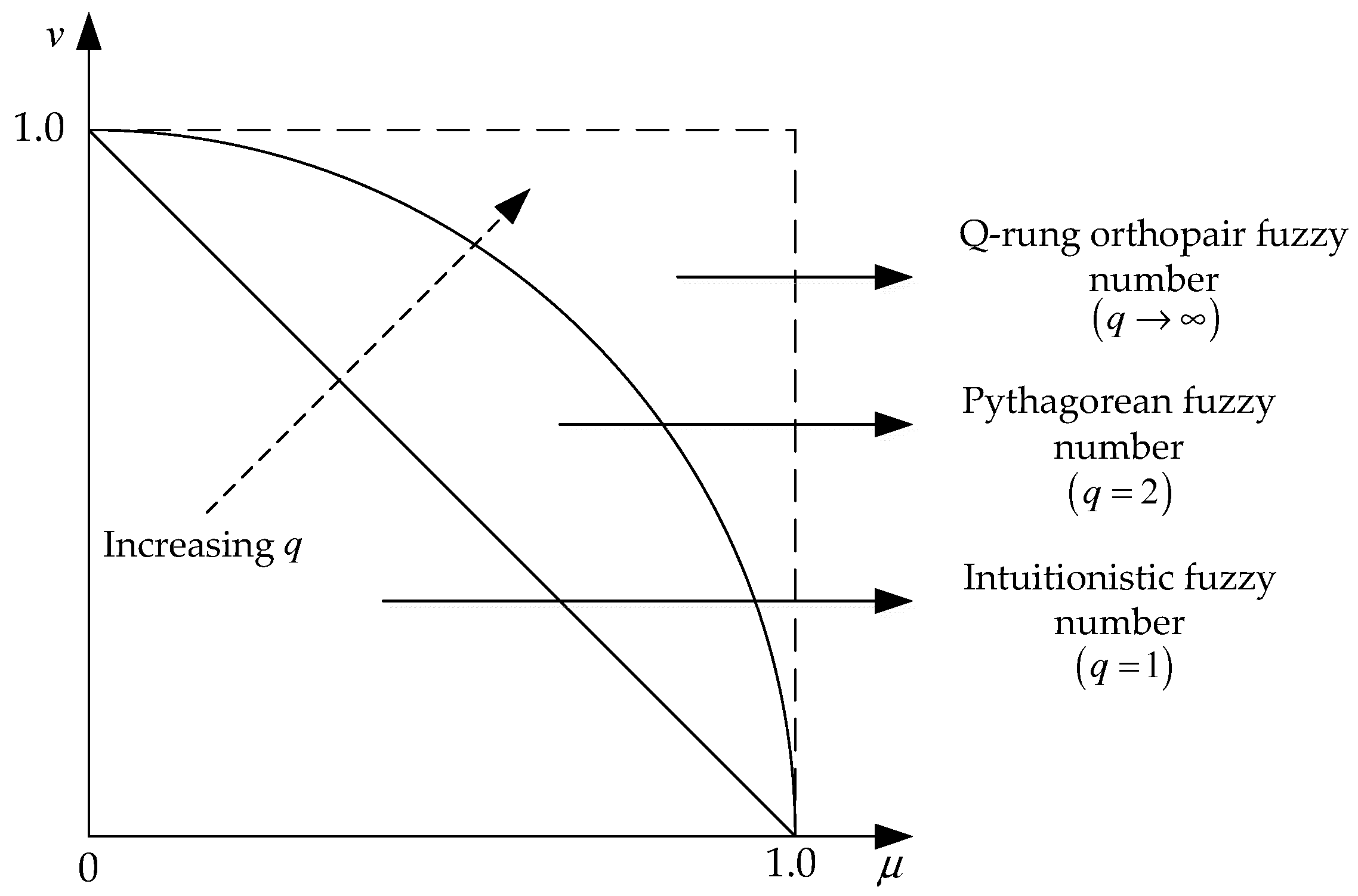
In practice, the related qualitative and quantitative data of green suppliers are always incomplete and complex; thus, crisp numbers cannot express the uncertainty of evaluation information given by decision makers. To solve this problem, Zadeh [44] developed the FS theory to represent the evaluation information; the generalized fuzzy numbers, including triangular fuzzy numbers and type-2 fuzzy numbers, were widely used in approaches for green supplier selection [8,14,33,41]. However, the FS ignores the non-membership degree of evaluation information. For instance, a business manager evaluates an investment before investing; they might think the probability of profit is 0.6, and the probability of loss is 0.3. Obviously, the FS cannot represent the aforementioned evaluation information. Therefore, Atanassov [45] applied the non-membership degree to improve the FS, and proposed the intuitionistic fuzzy set (IFS). Consequently, the evaluation information of the business manager can be expressed by an IFS, i.e., the membership and non-membership degrees are 0.6 and 0.3, respectively. Afterwards, IFS has been applied into green supplier selection [16,46]. Yager [47] proposed a generalized form of IFS called the Pythagorean fuzzy set (PFS), in which the sum of squares of membership and non-membership degrees is less than 1. Furthermore, to provide decision makers with a more relaxed evaluation environment, Yager [17] put forward the q-ROFS theory to express more potential evaluation information of decision makers. Then, the generalized form of q-ROFS, i.e., the q-rung picture linguistic set was proposed [48]. The q-ROFS theory can be regarded as a generalized form of IFS [45] and PFS [47], and the space of acceptable orthopairs increased with the increasing rung q as shown in Figure 1. Combined with the refusal membership degree, Cuong [49] developed the picture fuzzy set; subsequently, the similarity measures of the generalized picture fuzzy sets that including spherical fuzzy sets and T-spherical fuzzy sets were investigated [50]. However, picture fuzzy set is more applicable to model phenomena like voting.

2.3. Consensus Model

During the green supplier selection process, decision makers may come from different research fields of GSCM and have varying degrees of domain experience. Therefore, the non-consensus evaluation information, which is far from group opinions, will be inevitably revealed; however, a ranking result with a low consensus level may be obtained, which is not desirable. In recent years, the consensus model of MCGDM problems has been a hot topic. The existing consensus models can be divided into two categories; one is the iteration-based consensus model. For example, Herrera-Viedma et al. [51] defined the consensus and proximity measures of different preference structures to construct an iteration-based consensus support system. Herrera-Viedma et al. [52] investigated the consistency and consensus of incomplete fuzzy preference relations; a feedback mechanism was put forward to revise the consistency and consensus levels, simultaneously. With respect to intuitionistic fuzzy preference relations, Chu et al. [53] developed two iteration-based algorithms to improve the consistency and consensus levels, respectively. Wu et al. [54] put forward an iteration-based consensus model to revise the incomplete linguistic information, in which the trust degree was used to complete the decision matrices and adjust the weights of decision makers. Wu and Xu [55] developed a consensus measure of hesitant fuzzy linguistic information to complete the consensus-reaching process. Another kind of consensus model is the optimization-based consensus model. For instance, Dong et al. [56] constructed an optimization programming model for minimizing the number of adjusted simple terms to complete the consensus-reaching process under hesitant linguistic environment. Gong et al. [57] constructed two consensus models according to the minimum cost of consensus and maximum return to achieve a relatively high consensus level. Gong et al. [58] put forward a consensus model for optimizing the economic efficiency. Based on the multiplicative consistency, Xu et al. [59] and Zhang and Pedrycz [60] proposed goal programming models to improve the consistency and consensus levels of intuitionistic fuzzy preference and intuitionistic multiplicative preference relations, respectively. For green supplier selection issues, Zhu and Li [12] introduced a consensus model to put forward a novel green supplier selection approach; nevertheless, the consensus model can only provide suggestions to one of the decision makers for revising the non-consensus evaluation information in each iteration round, an thus, it can take a lot of time to achieve consensus in a complex environment.

2.4. The PA Operator

Based on the individual evaluation information, the collective information of each green supplier with respect to the criteria can be obtained by aggregation tools. Considering the relationships between the input information, Yager [26] developed the PA operator to aggregate the individual information. According to the PA operator and generalized weighted average operator, Zhou et al. [61] proposed the generalized power weighted average (GPWA) operator, in which the weight vectors were obtained by the subjective weight values and support degrees between different aggregated arguments. Xu [62] extended the PA operator into the intuitionistic fuzzy (IF) and interval-valued intuitionistic fuzzy environment; then, the generalized power weighted average operators were defined. Wan [63] put forward the MCGDM method by using a trapezoidal intuitionistic fuzzy power weighted average (TIFPWA) operator. Furthermore, Liu and Liu [64] investigated the generalized form of a TIFPWA operator. He et al. [65] discussed the properties of the interval-valued intuitionistic fuzzy power weighted average (IVIFPWA) operator and developed a novel MCGDM approach based on the IVIFPWA operator. According to the Frank operational laws, Zhang et al. [66] proposed a new form of PA operator. Wei and Lu [67] developed the Pythagorean fuzzy power weighted average (PFPWA) operator. To aggregate the q-rung orthopair fuzzy numbers (q-ROFNs), Liu et al. [27] extended the PA operator to the q-ROFPWA operator. Furthermore, the generalized PA operators have been applied to many practical areas to solve MCGDM problems [62,68,69,70,71].

3. Preliminaries

To make this paper as self-contained as possible, this section introduces the definition, operational laws, comparison method, Minkowski distance, and aggregation operator of q-ROFS, that will be utilized in the subsequent research.

3.1. q-ROFS

Based on the IFS and PFS, Yager [17] proposed a more general form, i.e., q-ROFS, and developed the operations of q-ROFS.

Definition 1 [17].

Let$\mathit{X}$be a non-empty and finite set, A q-ROFS$\mathit{Q}$on$\mathit{X}$ is defined by:

$$\mathit{Q}=\left\{\langle x,\left({\mu }_Q\left(x\right),v_Q\left(x\right)\right)\rangle |x\in \mathit{X}\right\},$$

(1)

where the functions ${\mu }_Q:\mathit{X}\to \left[0,1\right]$ and $v_Q:\mathit{X}\to \left[0,1\right]$ represent the membership and non-membership degrees of $x\in \mathit{X}$ to $\mathit{Q}$, respectively, and they satisfy the condition of ${\left({\mu }_Q\left(x\right)\right)}^q+{\left(v_Q\left(x\right)\right)}^q\le 1,q\ge 1$. Furthermore, function ${\pi }_Q\left(x\right)=\sqrt[q]{{\left({\mu }_Q\left(x\right)\right)}^q+{\left(v_Q\left(x\right)\right)}^q-{\left({\mu }_Q\left(x\right)\right)}^q{\left(v_Q\left(x\right)\right)}^q}$ indicates the indeterminacy membership degree. For convenience, we call $a=\left(\mu ,v\right)$ a q-ROFN.

Definition 2 [17].

Let$a=\left(\mu ,v\right)$,$a_1=\left({\mu }_1,v_1\right)$, and$a_2=\left({\mu }_2,v_2\right)$be three q-ROFNs,$\lambda >0$, and$a^c$is the complementary set of$a$, then:

$$a^c=\left(v,\mu \right);$$

(2)

$$a_1\oplus a_2=\left(\sqrt[q]{{\left({\mu }_1\right)}^q+{\left({\mu }_2\right)}^q-{\left({\mu }_1\right)}^q{\left({\mu }_2\right)}^q},v_1{v}_2\right);$$

(3)

$$a_1\otimes a_2=\left({\mu }_1{\mu }_2,\sqrt[q]{{\left(v_1\right)}^q+{\left(v_2\right)}^q-{\left(v_1\right)}^q{\left(v_2\right)}^q}\right);$$

(4)

$$\lambda a=\left(\sqrt[q]{1-{\left(1-{\mu }^q\right)}^{\lambda }},v^{\lambda }\right);$$

(5)

$$a^{\lambda }=\left({\mu }^{\lambda },\sqrt[q]{1-{\left(1-v^q\right)}^{\lambda }}\right).$$

(6)

Example 1.

Suppose that$a_1=\left(0.6500,0.8298\right)$and$a_2=\left(0.5000,0.7500\right)$are two q-ROFNs,$q=3$and$\lambda =2$, then:

(1) 

${\left(a_1\right)}^c=\left(0.8298,0.6500\right)$, ${\left(a_2\right)}^c=\left(0.7500,0.5000\right);$

(2) 

$a_1\oplus a_2=\left(0.7149,0.6224\right);$

(3) 

$a_1\otimes a_2=\left(0.3250,0.9094\right);$

(4) 

$\lambda a_1=\left(0.7796,0.6886\right)$, $\lambda a_2=\left(0.6166,0.5625\right);$

(5) 

${\left(a_1\right)}^{\lambda }=\left(0.4225,0.9346\right),{\left(a_2\right)}^{\lambda }=\left(0.2500,0.8732\right).$

Liu et al. [18] and Wei et al. [19] investigated the score and accuracy functions of q-ROFS, then, the comparison method of q-ROFNs was put forward.

Definition 3 [18,19].

Let$a=\left(\mu ,v\right)$be a q-ROFN, the score and accuracy functions of$a$are respectively given by:

$$s\left(a\right)=\left(1+{\mu }^q-v^q\right)/2;$$

(7)

$$h\left(a\right)={\mu }^q+v^q.$$

(8)

Definition 4 [19].

Let$a_1=\left({\mu }_1,v_1\right)$and$a_2=\left({\mu }_2,v_2\right)$be two q-ROFNs, then:

(1) 

If$s\left(a_1\right)<s\left(a_2\right)$, then$a_1<a_2$;

(2) 

If$s\left(a_1\right)=s\left(a_2\right)$, then

a.

$h\left(a_1\right)<h\left(a_2\right)$, then$a_1<a_2$;

b.

$h\left(a_1\right)=h\left(a_2\right)$, then$a_1=a_2$.

Later, Du [72] developed the Minkowski distance measure of q-ROFNs.

Definition 5 [72].

Let$a_1=\left({\mu }_1,v_1\right)$and$a_2=\left({\mu }_2,v_2\right)$be two q-ROFNs, then the Minkowski distance between them is defined by:

$$d\left(a_1,a_2\right)={\left(\frac{1}{2}{\left|{\mu }_1-{\mu }_2\right|}^p+\frac{1}{2}{\left|v_1-v_2\right|}^p\right)}^{1/p}.$$

(9)

Example 2.

Suppose that$a_1=\left(0.6500,0.8298\right)$and$a_2=\left(0.5000,0.7500\right)$are two q-ROFNs,$q=3$; according to Definition 3, we have$s\left(a_1\right)=s\left(a_2\right)=0.3516$,$h\left(a_1\right)=0.8460$, and$h\left(a_2\right)=0.5469$, then$a_1>a_2$. In addition, the Minkowski distance between them can be computed as$d\left(a_1,a_2\right)=0.1248$.

3.2. The q-ROFPWA Operator

Considering the relationship between the aggregated values, Yager [26] proposed the PA operator to fuse the information.

Definition 6 [26].

Let$a_i\left(i=1,2,\dots ,n\right)$be a collection of evaluation values, the PA operator is a mapping${\Omega }^n\to \Omega$as:

$$PA\left(a_1,a_2,\dots ,a_n\right)={\displaystyle \sum _{i=1}^n\frac{\left(1+T\left(a_i\right)\right)a_i}{{\displaystyle {\sum }_{j=1}^n\left(1+T\left(a_j\right)\right)}}}.$$

(10)

where$T\left(a_i\right)={\displaystyle {\sum }_{j=1,j\ne i}^{n}Sup\left(a_i,a_j\right)}$and$Sup\left(a_i,a_j\right)$is the support degree for$a_i$from$a_j$that satisfies the conditions as follows: (1)$Sup\left(a_i,a_j\right)\in \left[0,1\right];$(2)$Sup\left(a_i,a_j\right)=Sup\left(a_j,a_i\right);$(3) If$\left|a_i-a_j\right|>\left|a_s-a_t\right|$, then$Sup\left(a_i,a_j\right)\le Sup\left(a_s,a_t\right)$.

The PA operator can reflect the relationship between the aggregated values during the information fusion; however, it can only aggregate a crisp number. Therefore, Liu et al. [27] extended the PA operator into the q-ROF environment to propose the q-ROFPWA operator.

Definition 7 [27].

Let$a_i=\left({\mu }_i,v_i\right)\left(i=1,2,\dots ,n\right)$be a collection of q-ROFNs; the q-ROFPWA operator is a mapping${\Omega }^n\to \Omega$as:

$$q-ROFPWA\left(a_1,a_2,\dots ,a_n\right)=\underset{i=1}{\overset{n}{\oplus }}\frac{w_i\left(1+T\left(a_i\right)\right)a_i}{{\displaystyle {\sum }_{j=1}^n\left(w_j\left(1+T\left(a_j\right)\right)\right)}}.$$

(11)

where$\mathit{w}={\left(w_1,w_2,\dots ,w_n\right)}^T$is the weight vector of the q-ROFNs$a_i$,$T\left(a_i\right)={\displaystyle {\sum }_{j=1,j\ne i}^n\left(w_{j}Sup\left(a_i,a_j\right)\right)}$, and$Sup\left(a_i,a_j\right)=1-d\left(a_i,a_j\right)$is the support degree for$a_i$from$a_j$, in which$d\left(a_i,a_j\right)$is the Minkowski distance between$a_i$and$a_j$in this study.

Combined with the operations of q-ROFNs, we can obtain the following result.

Theorem 1 [27].

Let$a_i\left(i=1,2,\dots ,n\right)$be a collection of q-ROFNs; their aggregated value by using the q-ROFPWA operator is also a q-ROFN, and:

$$q-ROFPWA\left(a_1,a_2,\dots ,a_n\right)=\left(\sqrt[q]{1-{\displaystyle \prod _{i=1}^n{\left(1-{\mu }_i^q\right)}^{w_i\left(1+T\left(a_i\right)\right)/{\displaystyle {\sum }_{j=1}^n\left(w_j\left(1+T\left(a_j\right)\right)\right)}}}},{\displaystyle \prod _{i=1}^n{\left(v_i\right)}^{w_i\left(1+T\left(a_i\right)\right)/{\displaystyle {\sum }_{j=1}^n\left(w_j\left(1+T\left(a_j\right)\right)\right)}}}\right).$$

(12)

4. Green Supplier Selection Method under q-ROF Environment

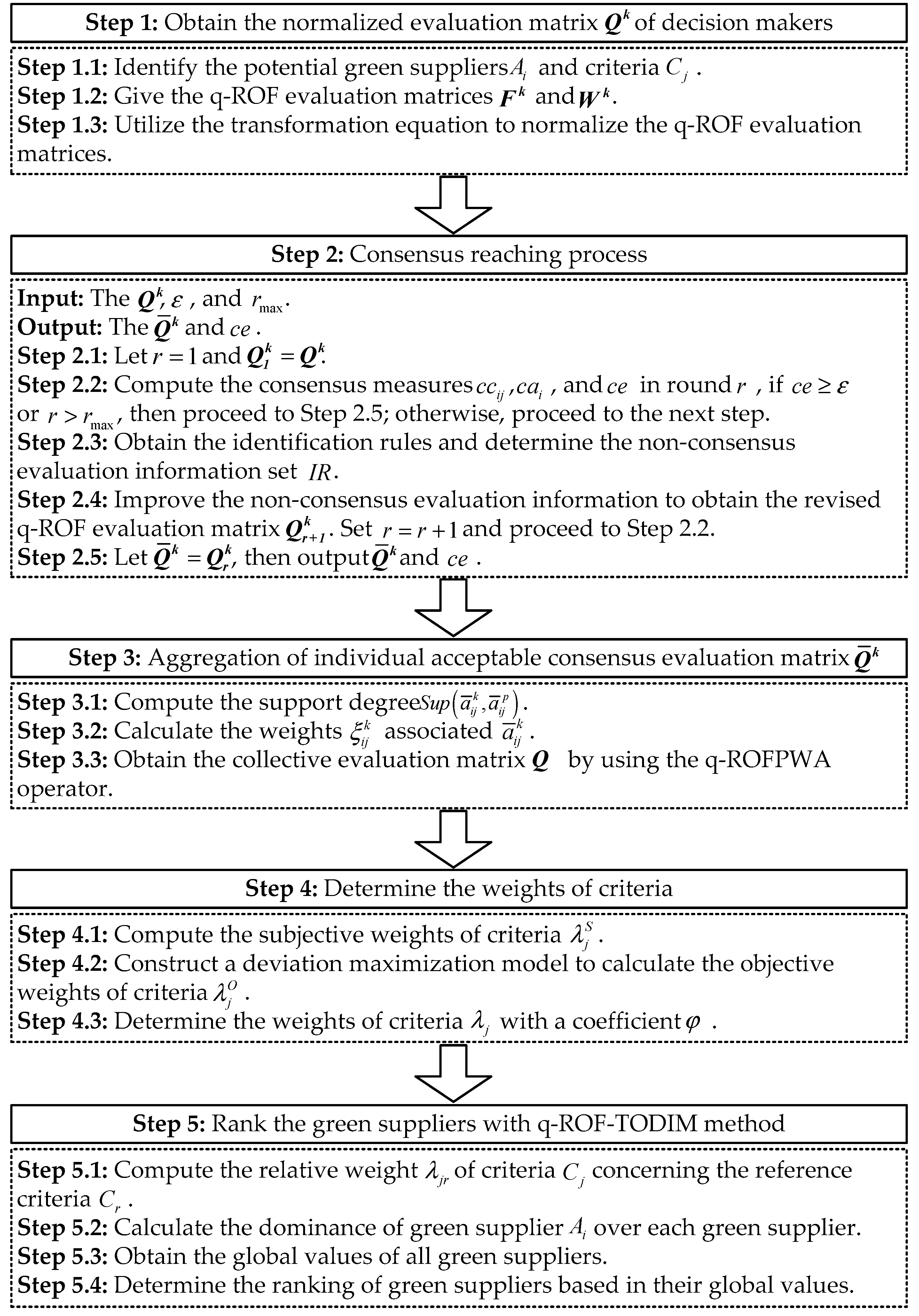
In this section, we defined the q-ROF consensus measures on three levels, namely, criteria, alternative, and evaluation matrix levels to construct the consensus model. Then, the q-ROFPWA operator was investigated to fuse the q-ROF evaluation information. Finally, combined with the comprehensive weighting method and q-ROF-TODIM method, a novel green supplier selection approach under q-ROF environment was developed. The flowchart of the proposed approach is presented in Figure 2.

4.1. Obtain the Normalized Evaluation Matrices of Decision Makers

For a green supplier selection problem, suppose that a group of decision makers $D_k\left(k=1,2,\dots ,l\right)$ is assembled to evaluate the green suppliers for an enterprise, in which decision makers may come from different backgrounds of GSCM. Then, the normalized q-ROF evaluation matrices of decision makers can be obtained by the steps as follows:

Step 1.1: After the primary evaluation of the green supplier selection problem, decision makers can identify the potential green supplier $A_i\left(i=1,2,\dots ,m\right)$ and a collection of criteria $C_j\left(j=1,2,\dots ,n\right)$.

Step 1.2: Combined with the q-ROFS, the evaluation information of green suppliers can be expressed by q-ROF evaluation matrix ${\mathit{F}}^{\mathit{k}}={\left({\tilde{a}}_{ij}^k\right)}_{m\times n}$, where ${\tilde{a}}_{ij}^k=\left({\tilde{\mu }}_{ij}^k,{\tilde{v}}_{ij}^k\right)$ indicates the q-ROF evaluation information of green supplier $A_i$ concerning criteria $C_j$ given by decision maker $D_k$. Moreover, decision makers also evaluate the weights of criteria using q-ROFNs; subsequently, the q-ROF evaluation matrix ${\mathit{W}}^{\mathit{k}}={\left(a_j^k\right)}_{1\times n}$ was obtained, where $a_j^k=\left({\mu }_j^k,v_j^k\right)$ represents the importance degree of criteria $C_j$ given by decision maker $D_k$.

Step 1.3: Generally, the criteria of green supplier selection can be divided into two types, namely, cost type and benefit type; thus, we should transform the information with respect to cost type criteria into the information with respect to benefit type criteria to determine the normalized q-ROF evaluation matrix ${\mathit{Q}}^{\mathit{k}}={\left(a_{ij}^k\right)}_{m\times n}$ as:

$$a_{ij}^k=\left({\mu }_{ij}^k,v_{ij}^k\right)=\{\begin{array}{ll}{\tilde{a}}_{ij}^k& \mathit{if}{C}_j\mathit{is}\mathit{the}\mathit{benefit}\mathit{type}\mathit{criteria};\\ {\left({\tilde{a}}_{ij}^k\right)}^c& \mathit{if}{C}_j\mathit{is}\mathit{the}\mathit{cost}\mathit{type}\mathit{criteria}.\end{array}$$

(13)

4.2. Consensus-Reaching Process

Most research focused on the consensus model with preference relations that were obtained by pairwise comparison; Wu and Xu [55] proposed an iteration-based consensus model to solve the MCGDM problems based on a hesitant fuzzy linguistic set. Motivated by the literature, we develop the similarity matrix between different q-ROF evaluation matrices.

Definition 8.

Suppose that decision maker$D_k\left(k=1,2,\dots ,l\right)$evaluated the alternative$A_i\left(i=1,2,\dots ,m\right)$concerning the criteria$C_j\left(j=1,2,\dots ,n\right)$using q-ROFNs. For each pair of decision makers,$\left(D_k,D_p\right)\left(k=1,2,\dots ,l-1;p=k+1,k+2,\dots ,l\right)$, the similarity matrix$\mathit{S}{\mathit{M}}^{\mathit{kp}}$between the q-ROF evaluation matrices${\mathit{Q}}^{\mathit{k}}={\left(a_{ij}^k\right)}_{m\times n}$and${\mathit{Q}}^{\mathit{p}}={\left(a_{ij}^p\right)}_{m\times n}$is defined by:

$$\mathit{S}{\mathit{M}}^{\mathit{kp}}={\left(s{m}_{ij}^{kp}\right)}_{m\times n}={\left(1-d\left(a_{ij}^k,a_{ij}^p\right)\right)}_{m\times n},$$

(14)

where$d\left(a_{ij}^k,a_{ij}^p\right)$is the Minkowski distance between the q-ROF evaluation information$a_{ij}^k$and$a_{ij}^p$. Furthermore, the consensus matrix$\mathit{CM}$is determined as:

$$\mathit{CM}={\left(c{m}_{ij}\right)}_{m\times n}={\left(\psi \left(s{m}_{ij}^{kp}\right)\right)}_{m\times n},$$

(15)

where$\psi$is the arithmetic average operator.

The three consensus measures on criteria, alternative, and evaluation matrix levels could then bedefined according to the consensus matrix $\mathit{CM}$, which will be used to complete the consensus-reaching process.

Definition 9.

Criteria level: the consensus measure$c{c}_{ij}$for alternative$A_i$with respect to criteria$C_j$can be represented by the element of consensus matrix$\mathit{CM}$as:

$$c{c}_{ij}=c{m}_{ij}.$$

(16)

Alternative level: the consensus measure$c{a}_i$on alternative$A_i$can be obtained by:

$$c{a}_i=\frac{{\displaystyle {\sum }_{j=1}^{n}c{c}_{ij}}}{n}.$$

(17)

Evaluation matrix level: the consensus measure$ce$on the evaluation matrix, i.e., the global consensus measure, can be defined by:

$$ce=\underset{i}{\min }\left\{c{a}_i\right\}.$$

(18)

Once the q-ROF consensus measures on three levels in Definition 9 were computed, we could check whether the consensus was achieved by comparing the consensus measure $ce$ with the predefined ideal consensus threshold $\epsilon \in \left(0,1\right]$. If $ce\ge \epsilon$, the consensus was reached; thus, the normalized q-ROF evaluation matrix ${\mathit{Q}}^{\mathit{k}}$ was the acceptable consensus evaluation matrix. Otherwise, several identification and direction rules could be obtained according to the aforementioned three consensus measures; identification rules were utilized to determine the non-consensus evaluation information set that contributed less to reach a high consensus level for each iteration round, and direction rules could guide decision makers to revise the non-consensus evaluation information in this round. An iteration-based consensus model under q-ROF environment was constructed to reach consensus as follows.

Input: The original individual evaluation matrix ${\mathit{Q}}^{\mathit{k}}$, the ideal consensus threshold $\epsilon$, and the maximum permission iterative number of times $r_{\max }$.

Output: The revised individual q-ROF evaluation matrix ${\overline{\mathit{Q}}}^{\mathit{k}}$ and the global consensus measure $ce$.

Step 2.1: Let the initial iterative number be $r=1$, and the individual evaluation matrix in the first round be ${\mathit{Q}}_{\mathbf{1}}^{\mathit{k}}={\left(a_{ij,1}^k\right)}_{m\times n}={\left(a_{ij}^k\right)}_{m\times n}$.

Step 2.2: Calculate the similarity matrix $\mathit{S}{\mathit{M}}^{\mathit{kp}}\left(k=1,2,\dots ,l-1;p=k+1,k+2,\dots ,l\right)$ and aggregate them to obtain the consensus matrix $\mathit{CM}$; thus, the consensus measures $c{c}_{ij}$, $c{a}_i$, and $ce$ in round $r$ are computed. If $ce\ge \epsilon$ or $r>r_{\max }$, then proceed to Step 1.5; otherwise, proceed to the next step.

Step 2.3: Obtain the identification rules as in the following:

(1) Identification rule 1. The non-consensus alternative set $IRA=\left\{A_i|c{a}_i<\epsilon ,i=1,2,\dots ,m\right\}$ identifies the rows of the evaluation matrices that should be revised.

(2) Identification rule 2. The non-consensus criteria set $IR{C}_i=\left\{C_j|A_i\in IRA\wedge c{c}_{ij}<\epsilon ,j=1,2,\dots ,n\right\}$ identifies the columns that should be revised for the rows distinguished in the non-consensus alternative set $IRA$.

(3) Identification rule 3. The non-consensus decision maker set $IR{D}_{ij}=\left\{D_p|A_i\in IRA\wedge C_j\in IR{C}_i\wedge d_{ij}^{\left(p\right)}=\underset{k}{\max }\left\{d_{ij}^{\left(k\right)}\right\}\right\}$ identifies the decision makers that should revise the evaluation information at the position $\left(i,j\right)$ in evaluation matrices, where $d_{ij}^{\left(p\right)}$ is the distance between the similarity measures of $D_p$ and other decision makers, i.e., $d_{ij}^{\left(p\right)}={\displaystyle {\sum }_{k=1,k\ne p}^l\left(1-s{m}_{ij}^{kp}\right)}$.

Subsequently, combined with the identification rules 1~3, the non-consensus evaluation information set $IR$ that should be revised in round $r$ can be determined as:

$$IR=\left\{\left(p,\left(i,j\right)\right)|D_p\in IR{D}_{ij}\wedge A_i\in IRA\wedge C_j\in IR{C}_i\right\}.$$

(19)

Step 2.4: Aggregate the individual evaluation matrix ${\mathit{Q}}_{\mathit{r}}^{\mathit{k}}$ using the q-ROFAA operator that is reduced by the q-ROFWA operator [18], then, the collective evaluation matrix ${\mathit{Q}}_{\mathit{r}}={\left(a_{ij,r}\right)}_{m\times n}$ can be obtained as:

$$a_{ij,r}=q-ROFAA\left(a_{ij,r}^1,a_{ij,r}^2,\dots ,a_{ij,r}^l\right)=\left(\sqrt[q]{1-{\displaystyle \prod _{k=1}^l{\left(1-{\left({\mu }_{ij,r}^k\right)}^q\right)}^{1/l}}},{\displaystyle \prod _{k=1}^l{\left(v_{ij,r}^k\right)}^{1/l}}\right).$$

(20)

Both the collective evaluation information $a_{ij,r}$ and the non-consensus evaluation information set $IR$ show that the direction rules, which suggest decision makers how to change their non-consensus evaluation information as in the following:

(1) If $a_{ij,r}>a_{ij,r}^k$, then the decision maker $D_k$ should decrease the evaluation on alternative $A_i$ concerning criteria $C_j$ when $C_j$ is the benefit type criteria, and the decision maker $D_k$ should increase the evaluation on alternative $A_i$ concerning criteria $C_j$ when $C_j$ is the cost type criteria.

(2) If $a_{ij,r}<a_{ij,r}^k$, the decision maker $D_k$ should increase the evaluation on alternative $A_i$ concerning criteria $C_j$ when $C_j$ is the benefit type criteria, and the decision maker $D_k$ should decrease the evaluation on alternative $A_i$ concerning criteria $C_j$ when $C_j$ is the cost type criteria.

Then, the revised individual q-ROF evaluation matrix ${\mathit{Q}}_{\mathit{r}\mathbf{+}\mathbf{1}}^{\mathit{k}}$ can be obtained. Set $r=r+1$ and proceed to Step 1.2.

Step 2.5: Let ${\overline{\mathit{Q}}}^{\mathit{k}}={\mathit{Q}}_{\mathit{r}}^{\mathit{k}}={\left({\overline{a}}_{ij}^k\right)}_{m\times n}={\left({\overline{\mu }}_{ij}^k,{\overline{v}}_{ij}^k\right)}_{m\times n}$. Output ${\overline{\mathit{Q}}}^{\mathit{k}}$ and $ce$ in this round.

4.3. Aggregation of Individual Acceptable Consensus Evaluation Matrices

According to the individual acceptable consensus evaluation matrices, we can use the q-ROFPWA operator to fuse them; then, the weights of decision makers can be determined by both the subjective weights and support degrees between individual evaluation information. Thus, the collective evaluation matrix $\mathit{Q}={\left(a_{ij}\right)}_{m\times n}$ is obtained by the steps as below.

Step 3.1: Compute the support degree:

$$Sup\left({\overline{a}}_{ij}^k,{\overline{a}}_{ij}^p\right)=1-d\left({\overline{a}}_{ij}^k,{\overline{a}}_{ij}^p\right),k,p=1,2,\dots ,l,$$

(21)

where $d\left({\overline{a}}_{ij}^k,{\overline{a}}_{ij}^p\right)$ is the Minkowski distance between the evaluation information ${\overline{a}}_{ij}^k$ and ${\overline{a}}_{ij}^p$.

Step 3.2: Combined with the subjective weight vector of decision makers $\mathit{w}={\left(w_1,w_2,\dots ,w_l\right)}^T$ that is provided by the enterprise, the weighted support degree of ${\overline{a}}_{ij}^k$ can be calculated as:

$$T\left({\overline{a}}_{ij}^k\right)={\displaystyle \sum _{p=1,p\ne k}^l{w}_{p}Sup\left({\overline{a}}_{ij}^k,{\overline{a}}_{ij}^p\right)},$$

(22)

Then, the weights associated with ${\overline{a}}_{ij}^k$ can be determined as:

$${\xi }_{ij}^k=\frac{w_k\left(1+T\left({\overline{a}}_{ij}^k\right)\right)}{{\displaystyle {\sum }_{k=1}^l\left(w_k\left(1+T\left({\overline{a}}_{ij}^k\right)\right)\right)}},{\xi }_{ij}^k\ge 0,{\displaystyle \sum _{k=1}^l{\xi }_{ij}^k=1.}$$

(23)

Step 3.3: Use the q-ROFPWA operator to fuse the evaluation matrix ${\overline{\mathit{Q}}}^{\mathit{k}}$ to obtain the collective evaluation matrix $\mathit{Q}$ as:

$$a_{ij}=q-ROFPWA\left({\overline{a}}_{ij}^1,{\overline{a}}_{ij}^2,\dots ,{\overline{a}}_{ij}^l\right)=\left(\sqrt[q]{1-{\displaystyle \prod _{k=1}^l{\left(1-{\left({\overline{\mu }}_{ij}^k\right)}^q\right)}^{{\xi }_{ij}^k}}},{\displaystyle \prod _{i=1}^n{\left({\overline{v}}_{ij}^k\right)}^{{\xi }_{ij}^k}}\right)=\left({\mu }_{ij},v_{ij}\right).$$

(24)

4.4. Determine the Weights of Criteria

In practice, it is sometimes unreasonable to determine the criteria weights only considering the views of decision makers. To investigate both the subjective and objective factors, we constructed a comprehensive weighting method that consists of a subjective weighting method and a deviation maximization model to calculate the weights of criteria as follows.

Step 4.1: Combined with the evaluation matrix ${\mathit{W}}^{\mathit{k}}$ and the similar steps in Section 4.3 and Section 4.4, we can obtain the collective evaluation matrix $\mathit{W}={\left(a_j\right)}_{1\times n}$. The larger the score value of $a_j$, which means the criteria $C_j$ is more important, the higher the weight of criteria $C_j$ and vice versa. Then, the subjective weight vector of criteria ${\mathit{\lambda }}^{\mathit{S}}={\left({\lambda }_1^S,{\lambda }_2^S,\dots ,{\lambda }_n^S\right)}^T$ can be determined as:

$${\lambda }_j^S=\frac{s\left(a_j\right)}{{\displaystyle {\sum }_{j=1}^{n}s\left(a_j\right)}}.$$

(25)

where $s\left(a_j\right)$ is the score value of $a_j$.

Step 4.2: Let ${\displaystyle {\sum }_{h=1,h\ne i}^{m}d\left(a_{ij},a_{hj}\right){\lambda }_j^O}$ be the deviation between the collective evaluation information on green supplier $A_i$ and other green suppliers concerning $C_j$, where $d\left(a_{ij},a_{hj}\right)$ is the Minkowski distance between $a_{ij}$ and $a_{hj}$; then, the total deviation is obtained as ${\displaystyle {\sum }_{j=1}^n{\displaystyle {\sum }_{i=1}^m{\displaystyle {\sum }_{h=1,h\ne i}^{m}d\left(a_{ij},a_{hj}\right){\lambda }_j^O}}}$. According to the information theory, if all green suppliers have similar evaluation information concerning one of criteria, a small weight value should be assigned to the criteria as it contributes less to differentiate green suppliers [73]. Subsequently, a deviation maximization model can be developed as:

$$\begin{array}{c}\max {\displaystyle {\sum }_{j=1}^n{\displaystyle {\sum }_{i=1}^m{\displaystyle {\sum }_{h=1,h\ne i}^{m}d\left(a_{ij},a_{hj}\right){\lambda }_j^O}}}\\ s.t.{\displaystyle {\sum }_{j=1}^n{\left({\lambda }_j^O\right)}^2=1,}{\lambda }_j^O\ge 0.\end{array}$$

(26)

Solve the model according to the Lagrange function:

$$L\left({\lambda }^O,\wp \right)={\displaystyle {\sum }_{j=1}^n{\displaystyle {\sum }_{i=1}^m{\displaystyle {\sum }_{h=1,h\ne i}^{m}d\left(a_{ij},a_{hj}\right){\lambda }_j^O}}}+\frac{\wp }{2}\left({\displaystyle {\sum }_{j=1}^n{\left({\lambda }_j^O\right)}^2-1}\right).$$

(27)

where $\wp$ is the Lagrange multiplier. Differentiate Equation (27) concerning ${\lambda }_j^O$ and $\wp$, and let these partial derivatives be equal to zero:

$$\{\begin{array}{l}\frac{\partial L\left({\lambda }^O,\wp \right)}{\partial {\lambda }_j^O}={\displaystyle {\sum }_{i=1}^m{\displaystyle {\sum }_{h=1,h\ne i}^{m}d\left(a_{ij},a_{hj}\right)}}+\wp {\lambda }_j^O=0;\\ \frac{\partial L\left({\lambda }^O,\wp \right)}{\partial \wp }={\displaystyle {\sum }_{j=1}^n{\left({\lambda }_j^O\right)}^2-1}=0.\end{array}$$

(28)

By solving Equation (28), the normalized weights of criteria, i.e., objective weight vector of criteria ${\mathit{\lambda }}^{\mathit{O}}={\left({\lambda }_1^O,{\lambda }_2^O,\dots ,{\lambda }_n^O\right)}^T$ can be obtained:

$${\lambda }_j^O=\frac{{\displaystyle {\sum }_{i=1}^m{\displaystyle {\sum }_{h=1,h\ne i}^{m}d\left(a_{ij},a_{hj}\right)}}}{{\displaystyle {\sum }_{j=1}^n{\displaystyle {\sum }_{i=1}^m{\displaystyle {\sum }_{h=1,h\ne i}^{m}d\left(a_{ij},a_{hj}\right)}}}}.$$

(29)

Step 4.3: Determine the comprehensive weight vector of criteria $\mathit{\lambda }={\left({\lambda }_1,{\lambda }_2,\dots ,{\lambda }_n\right)}^T$ as:

$${\lambda }_j=\phi {\lambda }_j^S+(1-\phi ){\lambda }_j^O.$$

(30)

where $\phi \in \left[0,1\right]$ is the importance coefficient of subjective weights, and $1-\phi$ is the importance coefficient of objective weights.

4.5. Rank the Green Suppliers Using the TODIM Method under q-ROF Environment

Based on the collective q-ROF evaluation matrix $\mathit{Q}$ and weight vector of criteria $\mathit{\lambda }$, we construct the q-ROF-TODIM method that can deal with the multiple criteria decision making problems with q-ROFS to obtain the ranking indices of green suppliers and determine the best green supplier.

Step 5.1: Compute the relative weight ${\lambda }_{jr}$ of criteria $C_j$ with respect to the reference criteria $C_r$ as:

$${\lambda }_{jr}={\lambda }_j/{\lambda }_r,$$

(31)

where ${\lambda }_j$ is the weight of criteria $C_j$ and ${\lambda }_r=\underset{j}{\max }\left\{{\lambda }_j\right\}$ is the weight of reference criteria $C_r$.

Step 5.2: Calculate the dominance degree of green supplier $A_i$ over each green supplier $A_h\left(h=1,2,\dots ,m\right)$ by the following equation:

$$\delta \left(A_i,A_h\right)={\displaystyle \sum _{j=1}^n{\varphi }_j\left(A_i,A_h\right)},$$

(32)

where:

$${\varphi }_j\left(A_i,A_h\right)=\{\begin{array}{ll}\sqrt{{\lambda }_{jr}d\left(a_{ij},a_{hj}\right)/{\displaystyle {\sum }_{j=1}^n{\lambda }_{jr}}}& if{a}_{ij}>a_{hj};\\ 0& if{a}_{ij}=a_{hj};\\ -\frac{1}{\theta }\sqrt{\left({\displaystyle {\sum }_{j=1}^n{\lambda }_{jr}}\right)d\left(a_{ij},a_{hj}\right)/{\lambda }_{jr}}& if{a}_{ij}<a_{hj}.\end{array}$$

(33)

The parameter $\theta$ $>$ $0$ indicates the attenuation factor of the losses, and $d\left(a_{ij},a_{hj}\right)$ is the Minkowski distance between $a_{ij}$ and $a_{hj}$.

Step 5.3: Compute the global value of green supplier $A_i$ by:

$$\Phi \left(A_i\right)=\frac{{\displaystyle {\sum }_{h=1}^m\delta \left(A_i,A_h\right)}-\underset{i}{\min }\left\{{\displaystyle {\sum }_{h=1}^m\delta \left(A_i,A_h\right)}\right\}}{\underset{i}{\max }\left\{{\displaystyle {\sum }_{h=1}^m\delta \left(A_i,A_h\right)}\right\}-\underset{i}{\min }\left\{{\displaystyle {\sum }_{h=1}^m\delta \left(A_i,A_h\right)}\right\}}.$$

(34)

Step 5.4: Determine the ranking of potential green suppliers based on their global values; the larger the global value $\Phi \left(A_i\right)$, the higher the ranking of green supplier $A_i$.

5. Numerical Example

In this section, a numerical example in the literature [16] was applied to show the feasibility and advantages of the proposed approach. An electric automobile enterprise plans to purchase a key component of a manufacturing procedure from the green suppliers market; the ranking of green suppliers can be determined by the following steps in the next subsection.

5.1. Implementation

Step 1: Obtain the normalized evaluation matrices of decision makers.

Step 1.1: After a preliminary evaluation, four potential green suppliers $A_i\left(i=1,2,3,4\right)$ are determined by a group of decision makers $D_k\left(k=1,2,3\right)$. Decision makers evaluate the four green suppliers concerning six criteria $C_j\left(j=1,2,3,4,5,6\right)$, namely, environmental costs ($C_1$), remanufacturing activity ($C_2$), energy assumption ($C_3$), reverse logistics program ($C_4$), hazardous waste management ($C_5$), and environmental certification ($C_6$), where $C_1$ and $C_3$ are the cost type criteria, and the others are the benefit type criteria.

Step 1.2: According to the relationships between the linguistic terms and interval-valued Pythagorean fuzzy numbers [74], we can construct the transformation between the linguistic terms and the corresponding q-ROFNs ($q=3$) as shown in

Table 1. Linguistic terms and the corresponding q-rung orthopair fuzzy numbers (q-ROFNs).

Linguistic Terms	Corresponding q-ROFNs
Extremely High (EH)	(0.95,0.15)
Very High (VH)	(0.85,0.25)
High (H)	(0.75,0.35)
Medium High (MH)	(0.65,0.45)
Medium (M)	(0.55,0.55)
Medium Low (ML)	(0.45,0.65)
Low (L)	(0.35,0.75)
Very Low (VL)	(0.25,0.85)
Extremely Low (EL)	(0.15,0.95)

. Then, decision makers use the linguistic terms to assess the green suppliers as shown in

Table 2. Evaluation information of decision makers.

Decision Makers	Alternatives	${\mathit{C}}_{\mathbf{1}}$	${\mathit{C}}_{\mathbf{2}}$	${\mathit{C}}_{\mathbf{3}}$	${\mathit{C}}_{\mathbf{4}}$	${\mathit{C}}_{\mathbf{5}}$	${\mathit{C}}_{\mathbf{6}}$
$D_1$	$A_1$	EH	H	L	EL	H	M
	$A_2$	MH	L	H	H	M	L
	$A_3$	L	H	M	L	EH	H
	$A_4$	L	EL	H	MH	MH	H
$D_2$	$A_1$	VH	VL	M	L	H	ML
	$A_2$	H	MH	MH	MH	M	ML
	$A_3$	L	VH	M	L	EL	H
	$A_4$	ML	H	H	MH	MH	H
$D_3$	$A_1$	ML	MH	ML	VL	VH	M
	$A_2$	VH	L	H	MH	MH	M
	$A_3$	ML	MH	MH	ML	EL	MH
	$A_4$	M	VH	EH	M	M	EL

; thus, the q-ROF evaluation matrix ${\mathit{F}}^{\mathit{k}}={\left({\tilde{a}}_{ij}^k\right)}_{4\times 6}$ is obtained. It is noteworthy that we adopt the subjective weights of criteria obtained in the literature [16], i.e., ${\mathit{\lambda }}^{\mathit{S}}={\left(0.180,0.090,0.130,0.130,0.310,0.160\right)}^T$.

Step 1.3: After the normalization step according to the different types of criteria, the normalized q-ROF evaluation matrix ${\mathit{Q}}^{\mathit{k}}={\left(a_{ij}^k\right)}_{4\times 6}$ can be obtained by using Equation (13).

Step 2: Consensus-reaching process ($\epsilon =0.85,r_{\max }=5$).

Step 2.1: Let the initial iterative number be $r=1$, and ${\mathit{Q}}_1^{\mathit{k}}={\left(a_{ij,1}^k\right)}_{4\times 6}={\left(a_{ij}^k\right)}_{4\times 6}$.

Step 2.2: Calculate the similarity matrix $\mathit{S}{\mathit{M}}^{\mathit{kp}}$ between the q-ROF evaluation matrices ${\mathit{Q}}_1^{\mathit{k}}$ and ${\mathit{Q}}_1^{\mathit{p}}$ as

$$\mathit{S}{\mathit{M}}^{12}=\left(\begin{array}{cccccc}0.9& 0.5& 0.8& 0.8& 1.0& 0.9\\ 0.9& 0.7& 0.9& 0.9& 1.0& 0.9\\ 1.0& 0.9& 1.0& 1.0& 0.2& 1.0\\ 0.9& 0.4& 1.0& 1.0& 1.0& 1.0\end{array}\right);\mathit{S}{\mathit{M}}^{13}=\left(\begin{array}{cccccc}0.5& 0.9& 0.9& 0.9& 0.9& 1.0\\ 0.8& 1.0& 1.0& 0.9& 0.9& 0.8\\ 0.9& 0.9& 0.9& 0.9& 0.2& 0.9\\ 0.8& 0.3& 0.8& 0.9& 0.9& 0.4\end{array}\right);\mathit{S}{\mathit{M}}^{23}=\left(\begin{array}{cccccc}0.6& 0.6& 0.9& 0.9& 0.9& 0.9\\ 0.9& 0.7& 0.9& 1.0& 0.9& 0.9\\ 0.9& 0.8& 0.9& 0.9& 1.0& 0.9\\ 0.9& 0.9& 0.8& 0.9& 0.9& 0.4\end{array}\right).$$

Then, aggregate them to obtain the consensus matrix $\mathit{CM}$ in round one:

$$\mathit{CM}=\left(\begin{array}{cccccc}0.6667& 0.6667& 0.8667& 0.8667& 0.9333& 0.9333\\ 0.8667& 0.8000& 0.9333& 0.9333& 0.9333& 0.8667\\ 0.9333& 0.8667& 0.9333& 0.9333& 0.4667& 0.9333\\ 0.8667& 0.5333& 0.8667& 0.9333& 0.9333& 0.6000\end{array}\right).$$

Thus, we can calculate the consensus measures $c{c}_{ij}$, $c{a}_i$, and $ce$ based on Equations (16)~(18); the global consensus measure in round one $ce=0.7889$. It can be seen that $ce<\epsilon$ after which we can proceed to the next step.

Step 2.3: Obtain the identification rules as in the following:

(1) Identification rule 1. The non-consensus alternative set: $IRA=\left\{A_i|c{a}_i<0.85\right\}=\left\{A_1,A_3,A_4\right\}.$

(2) Identification rule 2. The non-consensus criteria set:

$$IR{C}_1=\left\{C_j|A_1\in IRA\wedge c{c}_{1j}<0.85\right\}=\left\{C_1,C_2\right\};$$

$$IR{C}_3=\left\{C_j|A_3\in IRA\wedge c{c}_{3j}<0.85\right\}=\left\{C_5\right\};$$

$$IR{C}_4=\left\{C_j|A_4\in IRA\wedge c{c}_{4j}<0.85\right\}=\left\{C_2,C_6\right\}.$$

(3) Identification rule 3. Combined with the distances between the similarity measures of decision maker $D_p$ and the other decision makers at the positions $\left\{\left(1,1\right),\left(1,2\right),\left(3,5\right),\left(4,2\right),\left(4,6\right)\right\}$ in evaluation matrix ${\mathit{Q}}_1^{\mathit{k}}$, we can obtain the non-consensus decision maker set:

$$IR{D}_{11}=\left\{D_p|A_1\in IRA\wedge C_1\in IR{C}_1\wedge d_{11}^{\left(p\right)}=\underset{k}{\max }\left\{d_{11}^{\left(k\right)}\right\}\right\}=\left\{D_3\right\};$$

$$IR{D}_{12}=\left\{D_p|A_1\in IRA\wedge C_2\in IR{C}_1\wedge d_{12}^{\left(p\right)}=\underset{k}{\max }\left\{d_{12}^{\left(k\right)}\right\}\right\}=\left\{D_2\right\};$$

$$IR{D}_{35}=\left\{D_p|A_3\in IRA\wedge C_5\in IR{C}_3\wedge d_{35}^{\left(p\right)}=\underset{k}{\max }\left\{d_{35}^{\left(k\right)}\right\}\right\}=\left\{D_1\right\};$$

$$IR{D}_{42}=\left\{D_p|A_4\in IRA\wedge C_2\in IR{C}_4\wedge d_{42}^{\left(p\right)}=\underset{k}{\max }\left\{d_{42}^{\left(k\right)}\right\}\right\}=\left\{D_1\right\};$$

$$IR{D}_{46}=\left\{D_p|A_4\in IRA\wedge C_6\in IR{C}_4\wedge d_{46}^{\left(p\right)}=\underset{k}{\max }\left\{d_{46}^{\left(k\right)}\right\}\right\}=\left\{D_3\right\}.$$

Finally, based on the identification rules 1~3, the non-consensus evaluation information set $IR$ that should be revised in round one can be determined as:

$$IR=\left\{\left(p,\left(i,j\right)\right)|D_p\in IR{D}_{ij}\wedge A_i\in IRA\wedge C_j\in IR{C}_i\right\}=\left\{\left(3,\left(1,1\right)\right),\left(2,\left(1,2\right)\right),\left(1,\left(3,5\right)\right),\left(1,\left(4,2\right)\right),\left(3,\left(4,6\right)\right)\right\}.$$

Step 2.4: Aggregate the individual evaluation matrix ${\mathit{Q}}_1^{\mathit{k}}$ in round one using the q-ROFAA operator to obtain collective evaluation matrix ${\mathit{Q}}_1={\left(a_{ij,1}\right)}_{4\times 6}$; then, the direction rules can be put forward to revise the non-consensus evaluation information in set $IR$ as shown in

Table 3. Direction rules in round one.

$\mathit{I}\mathit{R}$	Individual Evaluation Information	Collective Evaluation Information	Direction Rules
(3,(1,1))	ML, (0.45,0.65)	(0.4750,0.7136)	ML→M
(2,(1,2))	VL, (0.25,0.85)	(0.6345,0.5116)	VL→L
(1,(3,5))	EH, (0.95,0.15)	(0.7823,0.5135)	EH→VH
(1,(4,2))	EL, (0.15,0.95)	(0.7332,0.4364)	EL→VL
(3,(4,6))	EL, (0.15,0.95)	(0.6745,0.4882)	EL→VL

. Set $r=2$ and proceed to Step 1.2.

Then, combined with the similar Steps 2.2~2.4, we can obtain the global consensus measure in round four $ce=0.8556>\epsilon$, which means that a high consensus level between decision makers has been achieved; the individual acceptable consensus q-ROF evaluation matrix ${\overline{\mathit{Q}}}^{\mathit{k}}$ are determined as shown in

Table 4. Individual acceptable consensus q-rung orthopair fuzzy (q-ROF) evaluation matrices.

Decision Makers	Alternatives	${\mathit{C}}_{\mathbf{1}}$	${\mathit{C}}_{\mathbf{2}}$	${\mathit{C}}_{\mathbf{3}}$	${\mathit{C}}_{\mathbf{4}}$	${\mathit{C}}_{\mathbf{5}}$	${\mathit{C}}_{\mathbf{6}}$
$D_1$	$A_1$	(0.15,0.95)	(0.75,0.35)	(0.75,0.35)	(0.15,0.95)	(0.75,0.35)	(0.55,0.55)
	$A_2$	(0.45,0.65)	(0.35,0.75)	(0.35,0.75)	(0.75,0.35)	(0.55,0.55)	(0.35,0.75)
	$A_3$	(0.75,0.35)	(0.75,0.35)	(0.55,0.55)	(0.35,0.75)	(0.85,0.25)	(0.75,0.35)
	$A_4$	(0.75,0.35)	(0.45,0.65)	(0.35,0.75)	(0.65,0.45)	(0.65,0.45)	(0.75,0.35)
$D_2$	$A_1$	(0.25,0.85)	(0.45,0.65)	(0.55,0.55)	(0.35,0.75)	(0.75,0.35)	(0.45,0.65)
	$A_2$	(0.35,0.75)	(0.65,0.45)	(0.45,0.65)	(0.65,0.45)	(0.55,0.55)	(0.45,0.65)
	$A_3$	(0.75,0.35)	(0.85,0.25)	(0.55,0.55)	(0.35,0.75)	(0.15,0.95)	(0.75,0.35)
	$A_4$	(0.65,0.45)	(0.75,0.35)	(0.35,0.75)	(0.65,0.45)	(0.65,0.45)	(0.75,0.35)
$D_3$	$A_1$	(0.45,0.65)	(0.65,0.45)	(0.65,0.45)	(0.25,0.85)	(0.85,0.25)	(0.55,0.55)
	$A_2$	(0.25,0.85)	(0.35,0.75)	(0.35,0.75)	(0.65,0.45)	(0.65,0.45)	(0.55,0.55)
	$A_3$	(0.65,0.45)	(0.65,0.45)	(0.45,0.65)	(0.45,0.65)	(0.15,0.95)	(0.65,0.45)
	$A_4$	(0.55,0.55)	(0.85,0.25)	(0.15,0.95)	(0.55,0.55)	(0.55,0.55)	(0.45,0.65)

.

Step 3: Aggregation of individual acceptable consensus evaluation matrices.

Steps 3.1~3.2: Suppose that the subjective weight values of decision makers are equal, i.e., $\mathit{w}={\left(1/3,1/3,1/3\right)}^T$; we can use Equations (21)~(23) to calculate the weighted support degree of ${\overline{a}}_{ij}^k$ as:

$${\mathit{T}}^1=\left(\begin{array}{cccccc}0.5333& 0.5333& 0.5667& 0.5667& 0.6333& 0.6333\\ 0.5667& 0.5667& 0.6333& 0.6000& 0.6333& 0.5667\\ 0.6333& 0.6000& 0.6333& 0.6333& 0.2000& 0.6333\\ 0.5667& 0.4333& 0.6000& 0.6333& 0.6333& 0.5667\end{array}\right);$$

$${\mathit{T}}^2=\left(\begin{array}{cccccc}0.5667& 0.5000& 0.5667& 0.5667& 0.6333& 0.6000\\ 0.6000& 0.4667& 0.6000& 0.6333& 0.6333& 0.6000\\ 0.6333& 0.5667& 0.6333& 0.6333& 0.4333& 0.6333\\ 0.6000& 0.5333& 0.6000& 0.6333& 0.6333& 0.5667\end{array}\right);$$

$${\mathit{T}}^3=\left(\begin{array}{cccccc}0.5000& 0.5667& 0.6000& 0.6000& 0.6000& 0.6333\\ 0.5667& 0.5667& 0.6333& 0.6333& 0.6000& 0.5667\\ 0.6000& 0.5667& 0.6000& 0.6000& 0.4333& 0.6000\\ 0.5667& 0.5000& 0.5333& 0.6000& 0.6000& 0.4667\end{array}\right).$$

Then, the weights associated with ${\overline{a}}_{ij}^k$ can be determined as:

$${\mathit{\xi }}^1=\left(\begin{array}{cccccc}0.3333& 0.3333& 0.3310& 0.3310& 0.3356& 0.3356\\ 0.3310& 0.3406& 0.3356& 0.3288& 0.3356& 0.3310\\ 0.3356& 0.3380& 0.3356& 0.3356& 0.2951& 0.3356\\ 0.3310& 0.3209& 0.3380& 0.3356& 0.3356& 0.3406\end{array}\right);$$

$${\mathit{\xi }}^2=\left(\begin{array}{cccccc}0.3406& 0.3261& 0.3310& 0.3310& 0.3356& 0.3288\\ 0.3380& 0.3188& 0.3288& 0.3356& 0.3356& 0.3380\\ 0.3356& 0.3310& 0.3356& 0.3356& 0.3308& 0.3356\\ 0.3380& 0.3333& 0.3380& 0.3356& 0.3356& 0.3406\end{array}\right);$$

$${\mathit{\xi }}^3=\left(\begin{array}{cccccc}0.3261& 0.3406& 0.3380& 0.3380& 0.3288& 0.3356\\ 0.3310& 0.3406& 0.3356& 0.3356& 0.3288& 0.3310\\ 0.3288& 0.3310& 0.3288& 0.3288& 0.3308& 0.3288\\ 0.3310& 0.3261& 0.3239& 0.3288& 0.3288& 0.3188\end{array}\right).$$

Step 3.3: Use the q-ROFPWA operator to fuse the evaluation matrix ${\overline{\mathit{Q}}}^{\mathit{k}}$ to obtain the collective evaluation matrix $\mathit{Q}$ as shown in

Table 5. Collective evaluation matrix.

Alternatives	${\mathit{C}}_{\mathbf{1}}$	${\mathit{C}}_{\mathbf{2}}$	${\mathit{C}}_{\mathbf{3}}$	${\mathit{C}}_{\mathbf{4}}$	${\mathit{C}}_{\mathbf{5}}$	${\mathit{C}}_{\mathbf{6}}$
$A_1$	(0.3331,0.8082)	(0.6512,0.4677)	(0.6660,0.4425)	(0.2747,0.8461)	(0.7904,0.3133)	(0.5221,0.5811)
$A_2$	(0.3692,0.7456)	(0.4985,0.6341)	(0.3893,0.7155)	(0.6888,0.4143)	(0.5883,0.5149)	(0.4665,0.6449)
$A_3$	(0.7225,0.3801)	(0.7690,0.3396)	(0.5221,0.5811)	(0.3893,0.7155)	(0.6271,0.6421)	(0.7225,0.3801)
$A_4$	(0.6660,0.4425)	(0.7415,0.3869)	(0.3116,0.8097)	(0.6220,0.4807)	(0.6220,0.4807)	(0.6926,0.4264)

.

Step 4: Determine the weights of the criteria.

Step 4.1: Because the subjective weights of criteria were determined in the literature [16], we adopt the subjective weight vector of criteria as ${\mathit{\lambda }}^{\mathit{S}}={\left(0.180,0.090,0.130,0.130,0.310,0.160\right)}^T$.

Step 4.2: Based on the collective evaluation matrix $\mathit{Q}$, we can construct the programming model, i.e., Equation (26); then, the objective weight vector of criteria can be determined as ${\mathit{\lambda }}^{\mathit{O}}={\left(0.201,0.160,0.150,0.182,0.151,0.156\right)}^T$.

Step 4.3: Set the importance coefficient of subjective weights to $\phi =0.5$; we can obtain the comprehensive weights of criteria as $\mathit{\lambda }={\left(0.191,0.125,0.140,0.156,0.230,0.158\right)}^T$.

Step 5: Rank the green suppliers using the TODIM method under a q-ROF environment ($\theta =1$).

Step 5.1: Utilize Equation (31) to compute the relative weight ${\lambda }_{jr}$ of criteria $C_j$ concerning the reference criteria $C_r$ as:

$${\lambda }_{1r}=0.8304,{\lambda }_{2r}=0.5435,{\lambda }_{3r}=0.6087,{\lambda }_{4r}=0.6783,{\lambda }_{5r}=1.0000,{\lambda }_{6r}=0.6870.$$

Step 5.2: Compute the dominance degree of green supplier $A_i$ over each green supplier:

$$\mathit{\delta }=\left(\begin{array}{cccc}0& -1.5220& -4.0821& -4.2886\\ -3.7277& 0& -4.7679& -4.0119\\ -1.3699& -1.2635& 0& -1.5385\\ -0.6062& -0.7501& -2.5158& 0\end{array}\right).$$

Step 5.3: Compute the global value of green supplier $A_i$ by Equation (34):

$$\Phi \left(A_1\right)=0.3028,\Phi \left(A_2\right)=0,\Phi \left(A_3\right)=0.9653,\Phi \left(A_4\right)=1.$$

Step 5.4: Based on the global values of green suppliers, the ranking of potential green suppliers can be determined as $A_4>A_3>A_1>A_2$. The green supplier $A_4$ is the best choice for the electric automobile company.

5.2. Comparison and Sensitivity Analysis

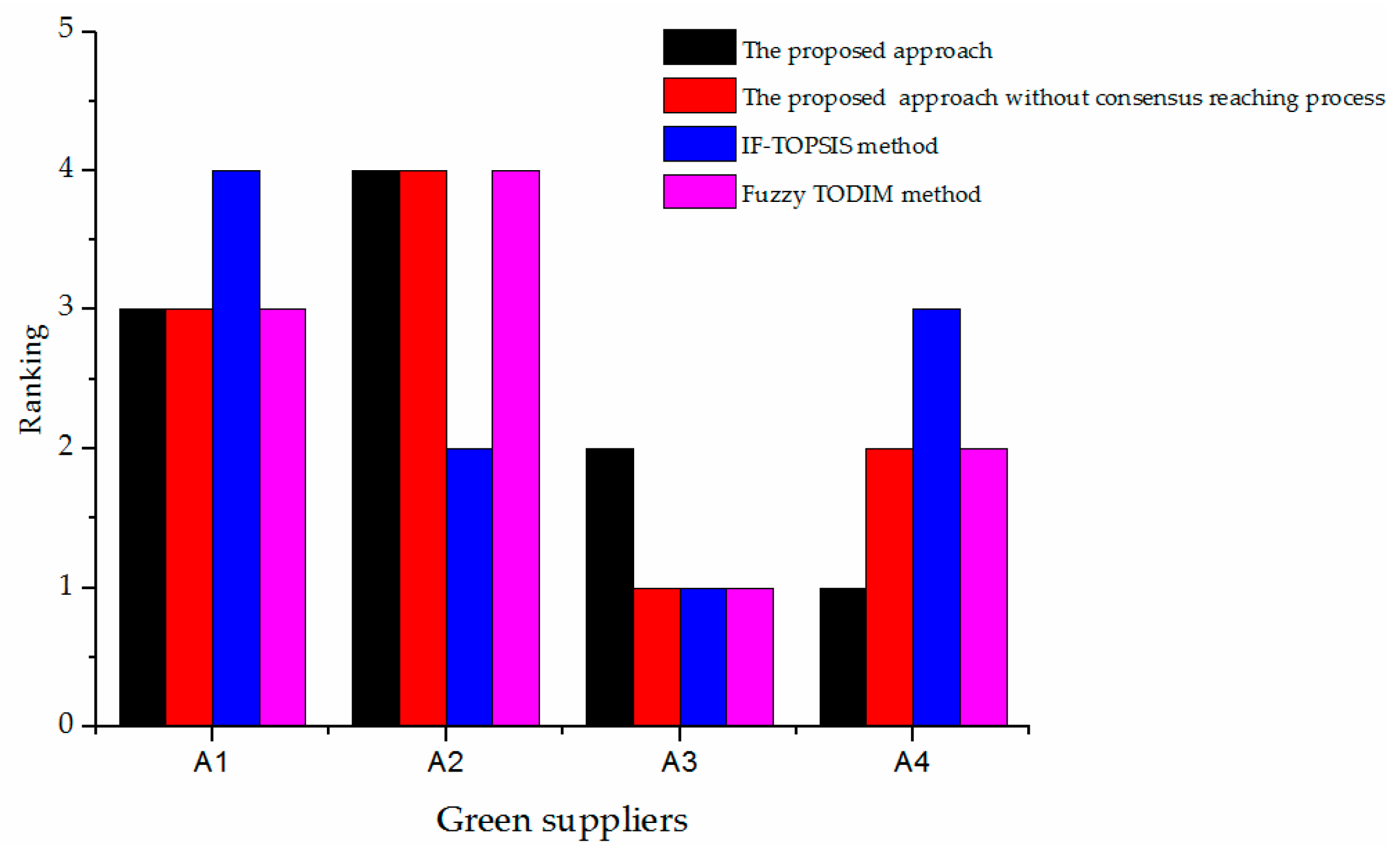
To investigate the influence of the consensus-reaching process on the ranking result and further verify the effectiveness of the proposed approach, we compared the ranking result of the green suppliers in Section 5.1 with the results that were obtained by the proposed approach without the consensus-reaching process, the green supplier selection approach based on the intuitionistic fuzzy TOPSIS (IF-TOPSIS) method [16], and the green supplier selection approach based on the fuzzy TODIM method [75]. The ranking results of the three green supplier selection approaches are shown in Figure 3; the detailed computation procedures of the proposed approach without consensus-reaching process, IF-TOPSIS method, and fuzzy TODIM method are presented in Appendix A, Appendix B and Appendix C, respectively.

The inconsistent ranking results between the proposed approach and the proposed approach without consensus-reaching process, i.e., the different ranking orders of green suppliers $A_3$ and $A_4$, can be explained by ignoring the consensus level of q-ROF evaluation information of decision makers. For instance, the linguistic term of decision maker $D_1$ for green supplier $A_3$ with respect to criteria $C_5$ was extremely low (EL); by contrast, the linguistic evaluation information of decision makers $D_2$ and $D_3$ for green supplier $A_3$ with respect to criteria $C_5$ were both extremely high (EH). Similarly, the linguistic terms of decision makers $D_1$ and $D_2$ for green supplier $A_4$ concerning criteria $C_6$ were both high (H); however, the linguistic evaluation information of decision maker $D_3$ for green supplier $A_4$ concerning criteria $C_6$ was EL. The aforementioned non-consensus evaluation information led to a change in the ranking orders of green suppliers $A_3$ and $A_4$ without a consensus-reaching process. In the procedures of the proposed approach, an iteration-based consensus model under a q-ROF environment was utilized to revise this non-consensus evaluation information until an acceptable consensus level between decision makers was achieved. Thus, we can obtain the ranking of green suppliers that was accepted by decision makers or enterprise; furthermore, the possible extreme evaluation information of individual decision maker was also revised to avoid affecting the accuracy of ranking result.

A notable difference existed between the rankings of the proposed method and IF-TOPSIS method. With the exception of ignoring the consensus problem between decision makers, the inconsistent result was caused by several other reasons. First, the evaluation information was represented by the q-ROFS in the proposed method, which is a generalized form of IFS that is used in the IF-TOPSIS method. Different basic data of green suppliers will lead to different result by aggregation tools. Second, combined with the q-ROFPWA operator, the decision maker weights were obtained by the subjective weights and support degrees between the evaluation information in the proposed approach; nevertheless, the determination of decision maker weights was omitted in the IF-TOPSIS method. Third, instead of the TOPSIS method, we utilized the q-ROF-TODIM method to determine the ranking of green suppliers. The q-ROF-TODIM method can consider the bounded rationality behavior of decision makers, which cannot be achieved by the TOPSIS method; consequently, the ranking result of green suppliers may differ.

From Figure 3, we can see that the ranking orders of green suppliers $A_3$ and $A_4$ were different between the rankings obtained by the proposed approach and fuzzy TODIM method. The main reason for this result is that the consensus-reaching process was omitted in the fuzzy TODIM method; the non-consensus evaluation information of decision makers made green supplier $A_3$ rank first in the ranking results determined by the proposed approach without a consensus-reaching process, IF-TOPSIS method, and fuzzy TODIM method. Moreover, the fuzzy TODIM method utilizes the triangular fuzzy numbers to express the evaluation information of decision makers, in which the non-membership and indeterminacy membership levels were ignored. The weights of decision makers in fuzzy TODIM method were assumed to be equal, which was inconsistent with the actual situation.

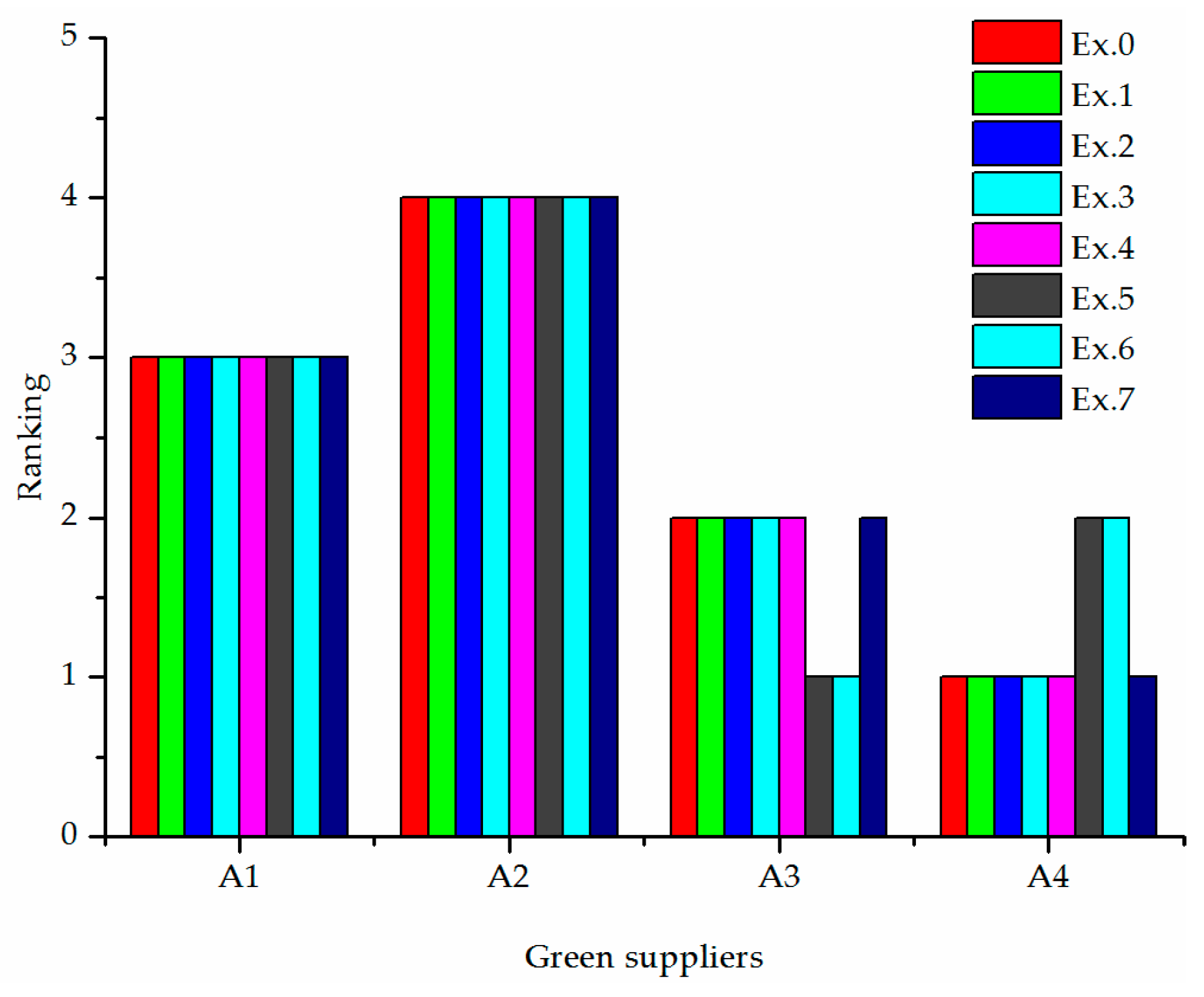
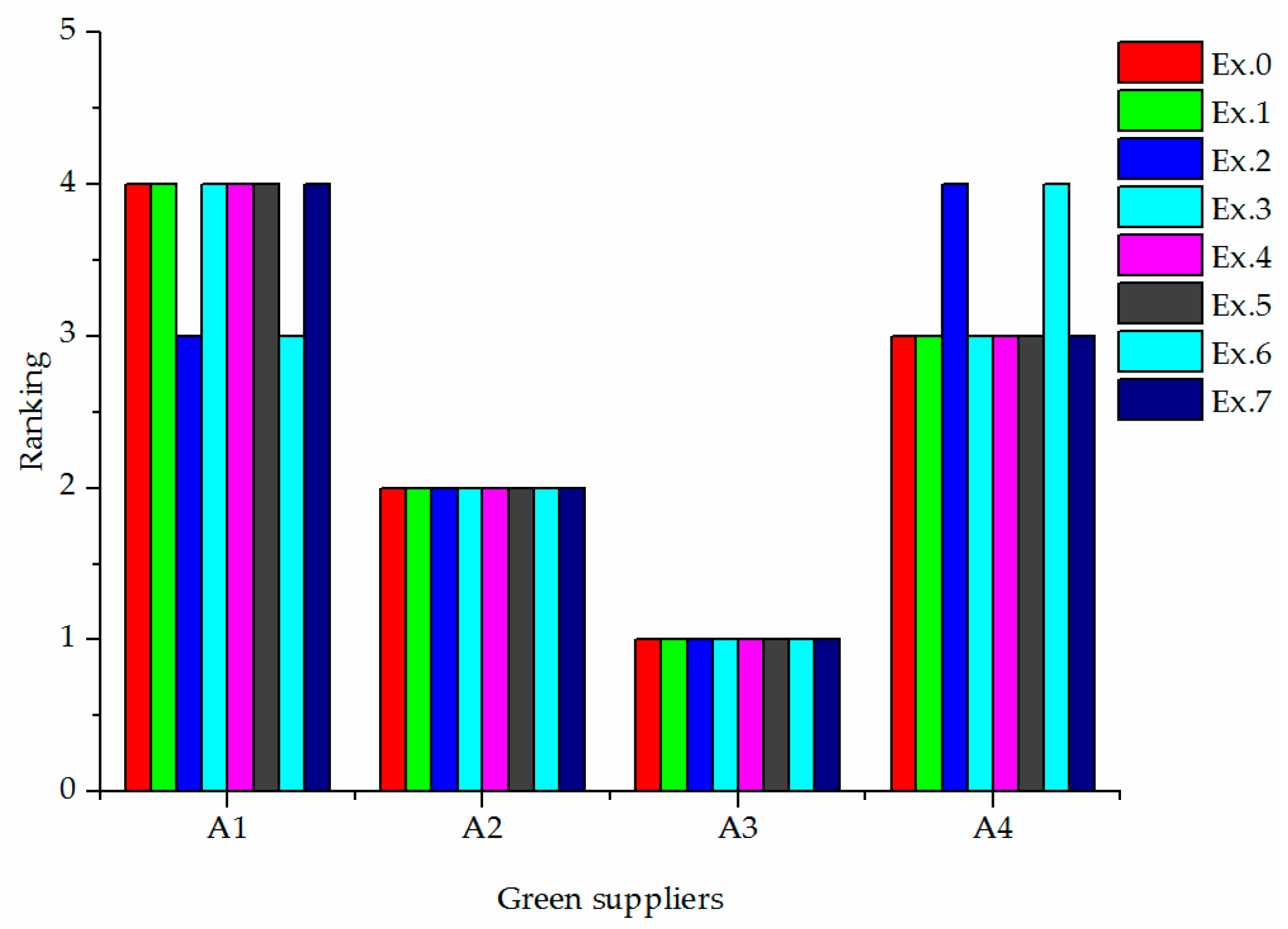
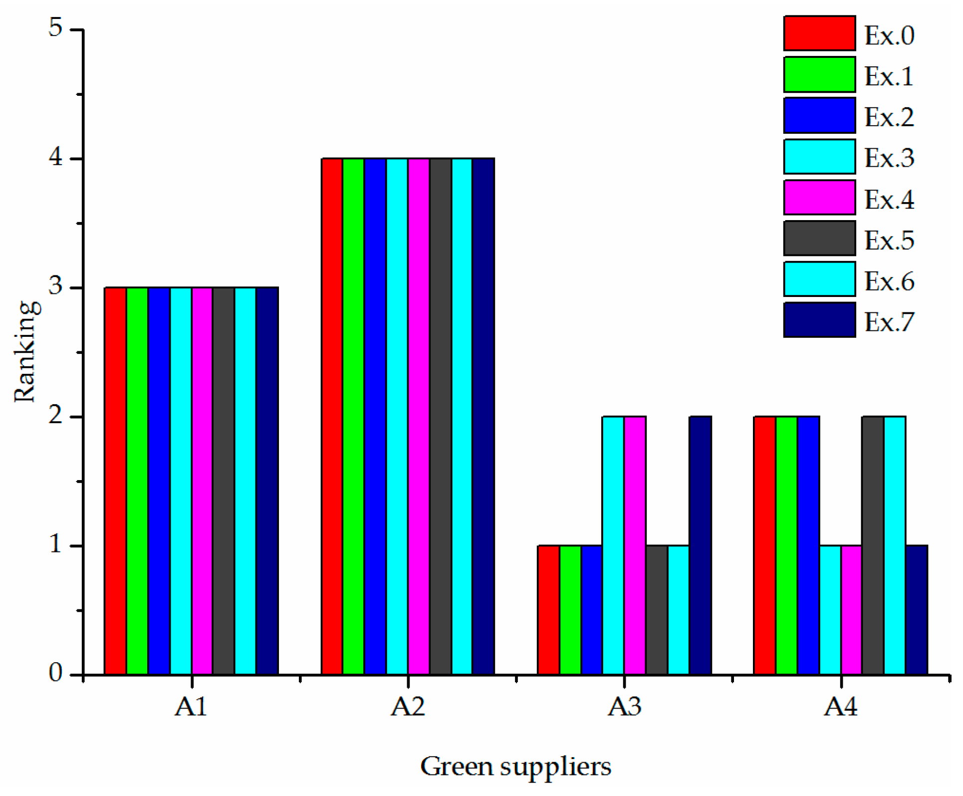
Furthermore, a sensitivity analysis was implemented by changing the weights of criteria as shown in

Table 6. Different weights of criteria in the sensitivity analysis.

Examples	${\mathit{C}}_{\mathbf{1}}$	${\mathit{C}}_{\mathbf{2}}$	${\mathit{C}}_{\mathbf{3}}$	${\mathit{C}}_{\mathbf{4}}$	${\mathit{C}}_{\mathbf{5}}$	${\mathit{C}}_{\mathbf{6}}$
Example 0	0.191	0.125	0.140	0.156	0.230	0.158
Example 1	1/6	1/6	1/6	1/6	1/6	1/6
Example 2	0.750	0.050	0.050	0.050	0.050	0.050
Example 3	0.050	0.750	0.050	0.050	0.050	0.050
Example 4	0.050	0.050	0.750	0.050	0.050	0.050
Example 5	0.050	0.050	0.050	0.750	0.050	0.050
Example 6	0.050	0.050	0.050	0.050	0.750	0.050
Example 7	0.050	0.050	0.050	0.050	0.050	0.750

. The rankings under different situations of the proposed approach, IF-TOPSIS method, and fuzzy TODIM method are illustrated in Figure 4, Figure 5 and Figure 6, respectively. Example 0 showed the weights of criteria that were determined by the proposed method, and Examples 1~7 showed the other possible weight values. From Table 6 and Figure 4, we can see that when the weight values of criteria $C_4$ and $C_5$ were relatively large, the best green supplier changed from $A_4$ to $A_3$, which means that the criteria weights play a crucial role in determining the ranking of green suppliers. Therefore, we should select the appropriate weighting method in practice. The comprehensive weighting approach in the proposed method considered the subjective and objective factors to obtain the more accurate weights of criteria. Once decision makers were confident for the evaluation information of criteria weights, the coefficient $\phi$ could be assigned a large value; otherwise, the coefficient $\phi$ could be assigned a small value. On the other hand, in addition to Examples 5 and 6, the rankings remain the same as $A_4>A_3>A_1>A_2$ under other situations; the proposed method is proven to be relatively insensitive to the weights of criteria.

The Spearman’s rank correlation coefficient is a powerful tool for measuring the similarity between rankings obtained by MCGDM methods [76]. To investigate the robustness of different green supplier selection approaches, combined with the rankings in Figure 4, Figure 5 and Figure 6, we can calculate the Spearman’s rank correlation coefficients between the ranking of Example 0 and the rankings of other possible weights of criteria, respectively. Thus, the average of these Spearman’s rank correlation coefficients can be utilized to measure the robustness of each green supplier selection approach, which are presented in

Table 7. Average of Spearman’s rank correlation coefficients of different approaches.

Methods	Average of Spearman’s Rank Correlation Coefficients
The proposed approach	0.9429
IF-TOPSIS method	0.9429
Fuzzy TODIM method	0.9143

. The larger the average of Spearman’s rank correlation coefficients, which means that the smaller the rankings change with different criteria weights, the stronger the robustness of this green supplier selection approach and vice versa. From Table 7, we can see that the robustness levels of all three green supplier selection approaches were relatively high, and the robustness of the proposed method and IF-TOPSIS was is slightly stronger than that of fuzzy TODIM method.

Based on the analysis above, the advantages of determining the best green supplier by using the proposed approach can be summarized as follows.

(1)

The q-ROFS is utilized to represent the evaluation information of decision makers, which can express the membership, non-membership, and indeterminacy membership degrees, simultaneously. Furthermore, with the increasing rung q, the space of acceptable orthopairs of q-ROFS is larger than IFS and PFS; as a generalized form of IFS and PFS, the proposed approach can also be transformed into other green supplier selection approaches under an IF and PF environment if necessary.

(2)

In practice, decision makers always differentiate from research fields and domain experiences; the non-consensus evaluation information of green suppliers will inevitably be given. Combined with an iteration-based consensus model under q-ROF environment, the non-consensus evaluation information of all the decision makers can be revised in each round. Therefore, a ranking of green suppliers accepted by decision makers or enterprises can be obtained using the proposed approach, and the efficiency of the consensus-reaching process is relatively high.

(3)

The q-ROFPWA operator is introduced to fuse the individual evaluation matrices; the weight vectors of decision makers can be determined by two aspects, namely, the subjective aspect and the objective aspect. Consequently, we can obtain a ranking of green suppliers that is closer to reality. Additionally, the determination of weights of decision makers is solved, which has been ignored by most existing approaches.

(4)

The weights of criteria are determined by a comprehensive weighting approach, which is composed of the subjective evaluation method and a deviation maximization model. Through changing the valve of coefficient $\phi$, the weights of the criteria can be determined; whether they are closer to subjective weights or objective weights depends on the choice of the decision makers or enterprises. Thus, the proposed approach is more able to cope with different scenarios.

(5)

During the green supplier evaluation process, the bounded rationality behavior of decision makers cannot be avoided. The TODIM method is a powerful tool to solve these MCGDM problems; in the proposed approach, the TODIM method is extended to the q-ROF environment to compute the ranking of green suppliers, which makes the evaluation result more realistic and accurate. In addition, the robustness of the proposed method is relatively strong.

The proposed approach also presents several limitations. With respect to the complicated green supplier selection issues, in which the number of evaluation criteria is relatively large; the interactions or dependencies between the criteria will inevitably exist. These situations cannot be solved combined with the proposed green supplier selection approach. Furthermore, decision makers may have difficulty determining the accurate value of a membership degree or linguistic term in real life. The proposed approach cannot deal with the issue of allowing decision makers to provide several possible values of different membership degrees or linguistic terms, which will be the focus of future research.

6. Conclusions

To deal with the complexity of green supplier selection problems in practice, this paper proposed a novel approach for green supplier selection under q-ROF environment. The q-ROFNs were utilized to express the evaluation information of decision makers; the uncertainty and incompleteness of the evaluation information were effectively addressed. Combined with the consensus measures on three levels, a q-ROF consensus model was developed to revise the non-consensus evaluation information of decision makers to improve the accuracy of the ranking results. To aggregate the q-ROF evaluation information of decision makers, the q-ROFPWA operator that considers both subjective and objective factors of decision maker weights was applied. Furthermore, a comprehensive weighting method was constructed to determine the weights of criteria, which consisted of the subjective weighting method and a deviation maximization model. Finally, the TODIM method under an q-ROF environment was proposed to obtain a ranking of potential green suppliers. An example of a green supplier selection problem in an electric automobile company was used to demonstrate the feasibility of the proposed method; subsequently, the effectiveness of the proposed method was illustrated by the sensitivity analysis and comparative analysis. In the case of increasingly complex green supplier selection issues, the proposed approach can deal with several aspects effectively, such as providing a relaxed evaluation environment for decision makers, promoting a relatively high consensus level between decision makers, and determining the weights of decision makers comprehensively. Thus, this paper provides a more reasonable and effective approach for enterprises to choose green suppliers in practice.

In future research, we will introduce the Choquet integral or Bonferroni mean operator to aggregate the evaluation information, which takes into account the relationships between the criteria. Furthermore, we can extend the proposed method into the q-rung orthopair hesitant fuzzy environment, in which decision makers have difficulty in determining the accurate membership and non-membership degrees.

References

- Sahu, N.K.; Datta, S.; Mahapatra, S.S. Establishing green supplier appraisement platform using grey concepts. Grey Syst. 2012, 2, 395–418. [Google Scholar] [CrossRef]
- Rostamzadeh, R.; Govindan, K.; Esmaeili, A.; Sabaghi, M. Application of fuzzy VIKOR for evaluation of green supply chain management practices. Ecol. Indic. 2015, 49, 188–203. [Google Scholar] [CrossRef]
- Vachon, S. Green supply chain practices and the selection of environmental technologies. Int. J. Prod. Res. 2007, 45, 4357–4379. [Google Scholar] [CrossRef]
- Cabral, I.; Grilo, A.; Cruz-Machado, V. A decision-making model for lean, agile, resilient and green supply chain management. Int. J. Prod. Res. 2012, 50, 4830–4845. [Google Scholar] [CrossRef]
- Beamon, B.M. Designing the green supply chain. Logist. Inf. Manag. 2013, 12, 332–342. [Google Scholar] [CrossRef]
- Bai, C.; Sarkis, J. Green supplier development: Analytical evaluation using rough set theory. J. Clean. Prod. 2010, 18, 1200–1210. [Google Scholar] [CrossRef]
- Wang, K.Q.; Liu, H.C.; Liu, L.; Huang, J. Green supplier evaluation and selection using cloud model theory and the QUALIFLEX method. Sustainability 2017, 9, 688. [Google Scholar] [CrossRef]
- Qin, J.D.; Liu, X.W.; Pedrycz, W. An extended TODIM multi-criteria group decision making method for green supplier selection in interval type-2 fuzzy environment. Eur. J. Oper. Res. 2017, 258, 626–638. [Google Scholar] [CrossRef]
- Kannan, D.; Govindan, K.; Rajendran, S. Fuzzy axiomatic design approach based green supplier selection: Acase study from singapore. J. Clean. Prod. 2015, 96, 194–208. [Google Scholar] [CrossRef]
- Blome, C.; Hollos, D.; Paulraj, A. Green procurement and green supplier development: Antecedents and effects on supplier performance. Int. J. Prod. Res. 2014, 52, 32–49. [Google Scholar] [CrossRef]
- Govindan, K.; Rajendran, S.; Sarkis, J.; Murugesan, P. Multi criteria decision making approaches for green supplier evaluation and selection: A literature review. J. Clean. Prod. 2015, 98, 66–83. [Google Scholar] [CrossRef]
- Zhu, J.H.; Li, Y.L. Green supplier selection based on consensus process and integrating prioritized operator and Choquet integral. Sustainability 2018, 10, 2744. [Google Scholar] [CrossRef]
- Wang, J.; Wei, G.W.; Wei, Y. Models for green supplier selection with some 2-tuple linguistic neutrosophic number Bonferroni mean operators. Symmetry 2018, 10, 131. [Google Scholar] [CrossRef]
- Banaeian, N.; Mobli, H.; Fahimnia, B.; Nielsen, I.E.; Omid, M. Green supplier selection using fuzzy group decision making methods: A case study from the agri-food industry. Comput. Oper. Res. 2017, 89, 337–347. [Google Scholar] [CrossRef]
- Ghorabaee, M.K.; Zavadskas, E.K.; Amiri, M.; Esmaeili, A. Multi-criteria evaluation of green suppliers using an extended WASPAS method with interval type-2 fuzzy sets. J. Clean. Prod. 2016, 137, 213–229. [Google Scholar] [CrossRef]
- Cao, Q.W.; Wu, J.; Liang, C.Y. An intuitionsitic fuzzy judgement matrix and TOPSIS integrated multi-criteria decision making method for green supplier selection. J. Intell. Fuzzy Syst. 2015, 28, 117–126. [Google Scholar] [CrossRef]
- Yager, R.R. Generalized orthopair fuzzy sets. IEEE Trans. Fuzzy Syst. 2017, 25, 1222–1230. [Google Scholar] [CrossRef]
- Liu, P.D.; Wang, P. Some q-rung orthopair fuzzy aggregation operators and their applications to multiple-attribute decision making. Int. J. Intell. Syst. 2018, 33, 259–280. [Google Scholar] [CrossRef]
- Wei, G.W.; Gao, H.; Wei, Y. Some q-rung orthopair fuzzy Heronian mean operators in multiple attribute decision making. Int. J. Intell. Syst. 2018, 33, 1426–1458. [Google Scholar] [CrossRef]
- Liu, P.D.; Liu, J.L. Some q-rung orthopair fuzzy Bonferroni mean operators and their application to multi-attribute group decision making. Int. J. Intell. Syst. 2018, 33, 315–347. [Google Scholar] [CrossRef]
- Alonso, S. A web based consensus support system for group decision making problems and incomplete preferences. Inf. Sci. 2010, 180, 4477–4495. [Google Scholar] [CrossRef]
- Chiclana, F.; Mata, F.; Martinez, L.; Herrera-Viedma, E.; Alonso, S. Integration of a consistency control module within a consensus model. Int. J. Uncertain. Fuzz. Knowl.-Based Syst. 2008, 16, 35–53. [Google Scholar] [CrossRef]
- Herrera-Viedma, E.; Cabrerizo, F.J.; Kacprzyk, J.; Pedrycz, W. A review of soft consensus models in a fuzzy environment. Inf. Fusion 2014, 17, 4–13. [Google Scholar] [CrossRef]
- Alcantud, J.C.R.; Calle, R.D.A.; Cascón, J.M. On measures of cohesiveness under dichotomous opinions: Some characterizations of approval consensus measures. Inf. Sci. 2013, 240, 45–55. [Google Scholar] [CrossRef]
- Alcantud, J.C.R.; Calle, R.D.A.; Cascón, J.M. A unifying model to measure consensus solutions in a society. Math. Comput. Model. 2013, 57, 1876–1883. [Google Scholar] [CrossRef]
- Yager, R.R. The power average operator. IEEE Trans. Syst. Man Cybern Part A Syst. Hum. 2001, 31, 724–731. [Google Scholar] [CrossRef]
- Liu, P.; Chen, S.M.; Wang, P. Multiple-attribute group decision-making based on q-rung orthopair fuzzy power maclaurin symmetric mean operators. IEEE Trans. Syst. Man Cybern. Syst. 2018, 1–16. [Google Scholar] [CrossRef]
- Gomes, L.F.A.M.; Lima, M.M.P.P. TODIM: Basic and application to multicriteria ranking of projects with environmental impacts. Found. Comput. Decis. Sci. 1991, 16, 113–127. [Google Scholar]
- Kahneman, D.; Tversky, A. Prospect theory: An analysis of decision under risk. Econometrica 1979, 47, 263–291. [Google Scholar] [CrossRef]
- Morente-Molinera, J.A.; Kou, G.; Crespo, R.G.; Corchado, J.M.; Herrera-Viedma, E. Solving multi-criteria group decision making problems under environments with a high number of alternatives using fuzzy ontologies and multi-granular linguistic modelling methods. Knowl.-Based Syst. 2017, 137, 54–64. [Google Scholar] [CrossRef]
- García-Díaz, V.; Espada, J.P.; Crespo, R.G.; G-Bustelo, B.C.P.; Lovelle, J.M.C. An approach to improve the accuracy of probabilistic classifiers fordecision support systems in sentiment analysis. Appl. Soft Comput. 2018, 67, 822–833. [Google Scholar] [CrossRef]
- Taibi, A.; Atmani, B. Combining fuzzy AHP with GIS and decision rules for industrial site selection. Int. J. Interact. Multimedia Artif. Intell. 2017, 4, 60–69. [Google Scholar] [CrossRef]
- Lee, A.H.I.; Kang, H.Y.; Hsu, C.F.; Hung, H.C. A green supplier selection model for high-tech industry. Expert Syst. Appl. 2009, 36, 7917–7927. [Google Scholar] [CrossRef]
- Chen, H.M.W.; Chou, S.Y.; Luu, Q.D.; Yu, H.K. A fuzzy MCDM approach for green supplier selection from the economic and environmental aspects. Math. Probl. Eng. 2016. [Google Scholar] [CrossRef]
- Yazdani, M. An integrated MCDM approach to green supplier selection. Int. J. Ind. Eng. Comput. 2014, 5, 443–458. [Google Scholar] [CrossRef]
- Tsui, C.W.; Wen, U.P. A hybrid multiple criteria group decision-making approach for green supplier selection in the TFT-LCD industry. Math. Probl. Eng. 2014. [Google Scholar] [CrossRef]
- Dobos, I.; Vörösmarty, G. Green supplier selection and evaluation using DEA-type composite indicators. Int. J. Prod. Econ. 2014, 157, 273–278. [Google Scholar] [CrossRef]
- Hashemi, S.H.; Karimi, A.; Tavana, M. An integrated green supplier selection approach with analytic network process and improved grey relational analysis. Int. J. Prod. Econ. 2015, 159, 178–191. [Google Scholar] [CrossRef]
- Kuo, R.J.; Wang, Y.C.; Tien, F.C. Integration of artificial neural network and MADA methods for green supplier selection. J. Clean. Prod. 2010, 18, 1161–1170. [Google Scholar] [CrossRef]
- Kuo, T.C.; Hsu, C.W.; Li, J.Y. Developing a green supplier selection model by using the DANP with VIKOR. Sustainability 2015, 7, 1661–1689. [Google Scholar] [CrossRef]
- Sang, X.Z.; Liu, X.W. An interval type-2 fuzzy sets-based TODIM method and its application to green supplier selection. J. Oper. Res. Soc. 2016, 67, 722–734. [Google Scholar] [CrossRef]
- Govindan, K.; Kadziński, M.; Sivakumar, R. Application of a novel PROMETHEE-based method for construction of a group compromise ranking to prioritization of green suppliers in food supply chain. Omega 2016, 71, 129–145. [Google Scholar] [CrossRef]
- Quan, M.Y.; Wang, Z.L.; Liu, H.C.; Shi, H. A hybrid MCDM approach for large group green supplier selection with uncertain linguistic information. IEEE Access 2018, 6, 50372–50383. [Google Scholar] [CrossRef]
- Zadeh, L.A. Fuzzy sets. Inf. Control 1965, 8, 338–353. [Google Scholar] [CrossRef] [Green Version]
- Atanassov, K.T. Intuitionistic fuzzy sets. Fuzzy Sets Syst. 1986, 20, 87–96. [Google Scholar] [CrossRef]
- Bali, O.; Kose, E.; Gumus, S. Green supplier selection based on IFS and GRA. Grey Syst. 2013, 3, 158–176. [Google Scholar] [CrossRef]
- Yager, R.R. Pythagorean membership grades in multicriteria decision making. IEEE Trans. Fuzzy Syst. 2014, 22, 958–965. [Google Scholar] [CrossRef]
- Li, L.; Zhang, R.T.; Wang, J.; Shang, X.P.; Bai, K.Y. A novel approach to multi-attribute group decision-making with q-rung picture linguistic information. Symmetry 2018, 10, 172. [Google Scholar] [CrossRef]
- Cường, B.C. Picture fuzzy sets. J. Comput. Sci. Cybern. 2014, 30, 409. [Google Scholar] [CrossRef]
- Ullah, K.; Mahmood, T.; Jan, N. Similarity measures for T-spherical fuzzy sets with applications in pattern recognition. Symmetry 2018, 10, 193. [Google Scholar] [CrossRef]
- Herrera-Viedma, E.; Herrera, F.; Chiclana, F. A consensus model for multiperson decision making with different preference structures. IEEE Trans. Syst. Man Cybern. Part A Syst. Hum. 2002, 32, 394–402. [Google Scholar] [CrossRef] [Green Version]
- Herrera-Viedma, E.; Alonso, S.; Chiclana, F.; Herrera, F. A consensus model for group decision making with incomplete fuzzy preference relations. IEEE Trans. Fuzzy Syst. 2007, 15, 863–877. [Google Scholar] [CrossRef]
- Chu, J.F.; Liu, X.W.; Wang, Y.M.; Chin, K.S. A group decision making model considering both the additive consistency and group consensus of intuitionistic fuzzy preference relations. Comput. Ind. Eng. 2016, 101, 227–242. [Google Scholar] [CrossRef]
- Wu, J.; Chiclana, F.; Herrera-Viedma, E. Trust based consensus model for social network in an incomplete linguistic information context. Appl. Soft Comput. 2015, 35, 827–839. [Google Scholar] [CrossRef] [Green Version]
- Wu, Z.B.; Xu, J.P. Possibility distribution-based approach for MAGDM with hesitant fuzzy linguistic information. IEEE Trans. Cybern. 2016, 46, 694–705. [Google Scholar] [CrossRef] [PubMed]
- Dong, Y.C.; Chen, X.; Herrera, F. Minimizing adjusted simple terms in the consensus reaching process with hesitant linguistic assessments in group decision making. Inf. Sci. 2015, 297, 95–117. [Google Scholar] [CrossRef]
- Gong, Z.W.; Zhang, H.H.; Forrest, J.; Li, L.S.; Xu, X.X. Two consensus models based on the minimum cost and maximum return regarding either all individuals or one individual. Eur. J. Oper. Res. 2015, 240, 183–192. [Google Scholar] [CrossRef]
- Gong, Z.W.; Xu, X.X.; Li, L.S.; Xu, C. Consensus modeling with nonlinear utility and cost constraints: A case study. Knowl.-Based Syst. 2015, 88, 210–222. [Google Scholar] [CrossRef]
- Xu, G.L.; Wan, S.P.; Wang, F.; Dong, J.Y.; Zeng, Y.F. Mathematical programming methods for consistency and consensus in group decision making with intuitionistic fuzzy preference relations. Knowl.-Based Syst. 2016, 98, 30–43. [Google Scholar] [CrossRef]
- Zhang, Z.M.; Pedrycz, W. Goal programming approaches to managing consistency and consensus for intuitionistic multiplicative preference relations in group decision-making. IEEE Trans. Fuzzy Syst. 2018. In press. [Google Scholar] [CrossRef]
- Zhou, L.G.; Chen, H.Y.; Liu, J.P. Generalized power aggregation operators and their applications in group decision making. Comput. Ind. Eng. 2012, 62, 989–999. [Google Scholar] [CrossRef]
- Xu, Z.S. Approaches to multiple attribute group decision making based on intuitionistic fuzzy power aggregation operators. Knowl.-Based Syst. 2011, 24, 749–760. [Google Scholar] [CrossRef]
- Wan, S.P. Power average operators of trapezoidal intuitionistic fuzzy numbers and application to multi-attribute group decision making. Appl. Math. Model. 2013, 37, 4112–4126. [Google Scholar] [CrossRef]
- Liu, P.D.; Liu, Y. An approach to multiple attribute group decision making based on intuitionistic trapezoidal fuzzy power generalized aggregation operator. Int. J. Comput. Intell. Syst. 2014, 7, 291–304. [Google Scholar] [CrossRef]
- He, Y.D.; Chen, H.Y.; Zhou, L.G.; Liu, J.P.; Tao, Z.F. Generalized interval-valued Atanassov’s intuitionistic fuzzy power operators and their application to group decision making. Int. J. Fuzzy Syst. 2013, 15, 401–411. [Google Scholar]
- Zhang, X.; Liu, P.D.; Wang, Y.M. Multiple attribute group decision making methods based on intuitionistic fuzzy Frank power aggregation operators. J. Intell. Fuzzy Syst. 2015, 29, 2235–2246. [Google Scholar] [CrossRef]
- Wei, G.W.; Lu, M. Pythagorean fuzzy power aggregation operators in multiple attribute decision making. Int. J. Intell. Syst. 2018, 33, 169–186. [Google Scholar] [CrossRef]
- Song, M.X.; Jiang, W.; Xie, C.H.; Zhou, D.Y. A new interval numbers power average operator in multiple attribute decision making. Int. J. Intell. Syst. 2017, 32, 631–644. [Google Scholar] [CrossRef]
- Liu, P.D.; Shi, L.L. The generalized hybrid weighted average operator based on interval neutrosophic hesitant set and its application to multiple attribute decision making. Neural Comput. Appl. 2015, 26, 457–471. [Google Scholar] [CrossRef]
- Xu, Y.J.; Merigó, J.M.; Wang, H.M. Linguistic power aggregation operators and their application to multiple attribute group decision making. Appl. Math. Model. 2012, 36, 5427–5444. [Google Scholar] [CrossRef]
- Wu, X.H.; Qian, J.; Peng, J.J.; Xue, C.C. A multi-criteria group decision-making method with possibility degree and power aggregation operators of single trapezoidal neutrosophic numbers. Symmetry 2018, 10, 590. [Google Scholar] [CrossRef]
- Du, W.S. Minkowski-type distance measures for generalized orthopair fuzzy sets. Int. J. Intell. Syst. 2018, 33, 802–817. [Google Scholar] [CrossRef]
- Xu, Z.S. A deviation-based approach to intuitionistic fuzzy multiple attribute group decision making. Group Decis. Negot. 2010, 19, 57–76. [Google Scholar] [CrossRef]
- Karaşan, A.; Ilbahar, E.; Cebi, S.; Kahraman, C. A new risk assessment approach: Safety and critical effect analysis (SCEA) and its extension with Pythagorean fuzzy sets. Saf. Sci. 2018, 108, 173–187. [Google Scholar] [CrossRef]
- Tosun, Ö.; Akyüz, G. A fuzzy TODIM approach for the supplier selection problem. Int. J. Comput. Intell. Syst. 2015, 8, 317–329. [Google Scholar] [CrossRef]
- Kou, G.; Lu, Y.Q.; Peng, Y.; Shi, Y. Evaluation of classification algorithms using MCDM and rank correlation. Int. J. Inf. Technol. Decis. Mak. 2012, 11, 197–225. [Google Scholar] [CrossRef]
- Xu, Z.S. Intuitionistic fuzzy aggregation operators. IEEE Trans. Fuzzy Syst. 2013, 14, 108–116. [Google Scholar] [CrossRef]
Figure 1.
Geometric space range of the intuitionistic fuzzy set (IFS), Pythagorean fuzzy set (PFS), and q-rung orthopair fuzzy set (q-ROFS).
Figure 2.
The flowchart of the proposed approach. Q-ROF: q-rung orthopair fuzzy. Q-ROFPWA: q-rung orthopair fuzzy power weighted average. Q-ROF-TODIM: q-rung orthopair fuzzy TOmada de Decisao Interativa e Multicritevio
Figure 3.
Ranking results of different approaches.
Figure 4.
Ranking results of the proposed approach with different weights of criteria.
Figure 5.
Ranking results of intuitionistic fuzzy (IF)-technique for order performance by similarity to ideal solution (TOPSIS) method with different weights of criteria.
Figure 6.
Ranking results of fuzzy TOmada de Decisao Interativa e Multicritevio (TODIM) method with different weights of criteria.