Random Untargeted Adversarial Example on Deep Neural Network †


1
School of Computing, Korea Advanced Institute of Science and Technology, Daejeon 34141, Korea
2
Department of Electrical Engineering, Korea Military Academy, Seoul 01805, Korea
3
Department of Medical Information, Kongju National University, Gongju-si 32588, Korea
*
Author to whom correspondence should be addressed.
†
Current address: KAIST, 291 Daehak-ro, Yuseong-gu, Daejeon 305-701, Korea.
†
This paper is an extended version of our paper published in MILCOM 2018.
Symmetry 2018, 10(12), 738; https://0-doi-org.brum.beds.ac.uk/10.3390/sym10120738
Submission received: 19 November 2018
/
Revised: 5 December 2018
/
Accepted: 9 December 2018
/
Published: 10 December 2018
Abstract
:Deep neural networks (DNNs) have demonstrated remarkable performance in machine learning areas such as image recognition, speech recognition, intrusion detection, and pattern analysis. However, it has been revealed that DNNs have weaknesses in the face of adversarial examples, which are created by adding a little noise to an original sample to cause misclassification by the DNN. Such adversarial examples can lead to fatal accidents in applications such as autonomous vehicles and disease diagnostics. Thus, the generation of adversarial examples has attracted extensive research attention recently. An adversarial example is categorized as targeted or untargeted. In this paper, we focus on the untargeted adversarial example scenario because it has a faster learning time and less distortion compared with the targeted adversarial example. However, there is a pattern vulnerability with untargeted adversarial examples: Because of the similarity between the original class and certain specific classes, it may be possible for the defending system to determine the original class by analyzing the output classes of the untargeted adversarial examples. To overcome this problem, we propose a new method for generating untargeted adversarial examples, one that uses an arbitrary class in the generation process. Moreover, we show that our proposed scheme can be applied to steganography. Through experiments, we show that our proposed scheme can achieve a 100% attack success rate with minimum distortion (1.99 and 42.32 using the MNIST and CIFAR10 datasets, respectively) and without the pattern vulnerability. Using a steganography test, we show that our proposed scheme can be used to fool humans, as demonstrated by the probability of their detecting hidden classes being equal to that of random selection.
1. Introduction
Command and control (C2) systems are being transformed into unmanned artificial intelligence systems with the development of informational operating paradigms for unmanned aerial vehicles, scientific monitoring systems, and surveillance systems. Artificial intelligence technology plays an important role in networks for enhancing such unmanned scientific monitoring systems. In particular, deep neural networks (DNNs) [1] provide superior performance for services such as image recognition, speech recognition, intrusion detection, and pattern analysis.
However, Szegedy et al. [2] introduced the concept of an adversarial example in image recognition: An image that is transformed slightly so it will be incorrectly classified by a DNN even when the changes are too small to be easily recognized by humans. Such adversarial examples are a serious threat to DNNs. For example, if an adversarial example is applied to a right-turn sign image so that it will be misclassified by a DNN as a U-turn sign image, an autonomous vehicle with a DNN may incorrectly classify the modified right-turn sign as a U-turn sign, whereas a human would correctly classify the modified sign as a right-turn sign.
Adversarial examples are divided into two categories according to the purpose of their generation: Targeted adversarial examples and untargeted adversarial examples. The purpose of generating a targeted adversarial example is to cause the target model to classify the adversarial example as a specific class chosen by the attacker, whereas the purpose of generating an untargeted adversarial example is to cause the target model to classify the adversarial example as any wrong class. Because the untargeted adversarial example has faster learning time and less distortion than the targeted adversarial example, our study focuses on the untargeted adversarial example. However, there is a disadvantage associated with the untargeted adversarial example, called pattern vulnerability. This is because certain classes will have higher similarity to the original sample; for example, in MNIST [3], the original sample “7” is similar to the “9” image, so an untargeted adversarial example based on the original sample “7” is more likely to be misclassified as the “9” class. This pattern vulnerability allows the original class used in generating the untargeted adversarial example to be accurately detected by analyzing the similarity between the original class and the specific classes.
To overcome the pattern vulnerability problem, we propose a random untargeted adversarial example in this paper. The proposed scheme uses a random class other than the original class when generating an untargeted adversarial example. This paper is an extended version of our previous work [4] presented at the Military Communications (MILCOM) 2018 conference. For MILCOM 2018, we focused on methods for generating a random untargeted adversarial example. The contributions of this paper are as follows.
- We systematically organize the framework of the proposed scheme. We present the random untargeted adversarial example and use it to verify the usefulness of a steganography [5] scheme and evaluate its security.
- We analyze the confusion matrix of the untargeted adversarial example and the proposed scheme in order to analyze recognition classes by each original class. We also analyze the recognition and detection rates of the proposed technique, using human subjects to test the method’s application to steganography.
- Through an experiment using the MNIST and CIFAR10 [6] datasets, we show the effectiveness of our proposed method. In addition, we point out the possibility of applying the proposed method to steganography without the pattern vulnerability.
The remainder of this paper is structured as follows. In Section 2, we review the related work and background: Section 2.1 describes neural networks, Section 2.2 describes the principle of generating adversarial examples, Section 2.3, Section 2.4, Section 2.5 and Section 2.6 describe the four ways adversarial example attacks are categorized (by target model information, recognition target for the adversarial example, distance measure, and generation method), and Section 2.7 describes the latest methods used by different models to recognize different classes. The problem definition is addressed in Section 3, and our proposed scheme is presented in Section 4. Section 5 describes the experiments and provides evaluations, and a steganography evaluation is presented in Section 6. Section 7 discusses the proposed method. Finally, conclusions are presented in Section 8.
2. Background and Related Work
Several issues have been discussed by Barreno et al. [7] regarding security in machine learning. They classified machine learning attacks into causative attacks [8] and exploratory attacks [2]. Causative attacks affect the training process of the machine by adding malicious training data to attack the machine. Exploratory attacks, on the other hand, cause misclassification by the machine, but they do not affect the training process of the machine. In terms of assumptions, an exploratory attack is more realistic than a causative attack because gaining access to training data is not easy. As a well-known type of exploratory attack, the adversarial example [2] threatens the security of the neural network. The first research on adversarial examples was performed by Szegedy et al. [2]. The purpose of the adversarial example is to cause a misclassification by the DNN; a human, however, will be unable to tell the difference between the adversarial example and the original sample.
2.1. Neural Networks
A neural network [1] is a combination of synapses that form a network; a neuron changes the synaptic bond strength through learning.
Such a structure is typically used when estimating and approximating functions obscured by many input and activation functions, as shown in Figure 1. It is usually represented as an interconnection of neural systems suitable for calculating values from inputs and performing machine learning such as for pattern recognition. For example, a neural network for image recognition is defined as having a set of input neurons that are activated by the pixels of the input image. After the variants and weights of the function are applied, activation of the neurons is transferred to other neurons. This process is repeated until the last output neuron is activated. The output is determined when the image is read.
2.2. Adversarial Example Generation
To generate an adversarial example, the transformer element needs a target model, an original sample x, and the original class y. First, the transformer accepts the original sample x and the original class y as input data. The transformer then generates a transformed example by adding a little noise w to the original sample x. The transformer provides the generated example to the target model and receives the class probability results for that as feedback. According to this feedback, the transformer modifies by adjusting w. To optimally minimize distortion distances between and x, the transformer repeats the above process while optimally adjusting the minimum noise value w until the other class probability is higher than the original class probability.
2.3. Categorization by Target Model Information
Adversarial examples fall into one of two categories, white-box [2,9,10] or black-box [2,11,12] attacks, depending on the amount of information available about the target model. It is considered a white-box attack when the attacker possesses detailed information about the target model’s parameters, architecture, and output class probabilities. Therefore, white-box attacks have almost 100% attack success. Some recent articles [13] have shown that it is very difficult to defend DNNs against white-box attacks [14,15].
On the other hand, it is considered a black-box attack when the attacker can only know the output value of the target model against the input value and does not possess the target model information. There are two representative types of black-box attack: the transfer attack [2,12] and the substitute network attack [11]. The first type, the transfer attack [2], is based on the fact that an adversarial example generated by an arbitrary local model can attack other models as well. A variety of studies [16,17] have been conducted using the transferability concept. In order to improve the transferability, researchers [18] have recently proposed an ensemble method that uses several models to attack other models. The second representative type, the substitute method, repeats the query process to create a substitute network similar to the target model. Once an alternative network is created, a white-box attack is possible using this new network.
2.4. Categorization by Recognition Target for Adversarial Example
Adversarial examples fall into two categories, targeted adversarial examples and untargeted adversarial examples, according to the recognition target for the adversarial example. A targeted adversarial example is designed to induce the target model to recognize the adversarial image as the target class chosen by the attacker. The targeted adversarial example is mathematically expressed as follows: Given original sample , target class , and a target model, we solve the optimization problem to determine a targeted adversarial example :
where means the distance between transformed example and original sample x, is the target class, is the x value that minimizes the function , and class results for the input values is provided by an operation function .
On the other hand, an untargeted adversarial example allows the target model to recognize the adversarial image as any wrong class, that is, any class other than the original class. The untargeted adversarial example is mathematically expressed as follows: Given original sample , original class y, and a target model, we solve the optimization problem to determine an untargeted adversarial example :
The targeted adversarial example is a sophisticated attack that allows an attacker to control the perception of the class to the attacker’s choice. However, the untargeted adversarial example has the advantage of shorter learning time and less distortion compared to the targeted adversarial example.
2.5. Categorization by Distance Measure
There are three formulas for measuring the distance between the original sample and the adversarial example [9,13]: , , and . The first, , represents the sum of all changed pixels:
where is the pixel of the adversarial example and is the pixel of the original sample. The second, , is the Euclidean standard, meaning the sum of the square roots of the squared differences between each pair of corresponding pixels, as follows:
The third, , means the maximum distance between and among all pixels.
Because it depends on the case, it is difficult to make a general statement about which of the three methods is superior. However, the smaller the values of the three distance measures, the greater the similarity between the original sample and the adversarial example.
2.6. Methods of Adversarial Example Attack
There are four representative methods of creating adversarial examples: The fast-gradient sign method (FGSM) [19], iterative FGSM (I-FGSM) [20], the Deepfool method [10], and the Carlini & Wagner (CW) method [9]. The first, FGSM, uses the distance measure to generate adversarial example . This method is simple and effective.
where t is a target class, F is an operation function, and is the loss function based on t and F. The gradient of the loss function must be calculated because the loss function is minimized when the gradient of the loss function is minimized. At each iteration of the FGSM, the gradient is optimally minimized by updating from the original x, and is retrieved by optimization.
The second, I-FGSM, is an updated version of FGSM. At every step, the value of in FGSM is further refined, so a smaller amount called is updated, and this value is eventually clipped by the same .
where performs per-pixel clipping of the input; it is a function that subdivides the clipped area in order to prevent a large change. I-FGSM has improved performance over FGSM.
The third, the Deepfool method, uses the distance measure to generate an untargeted adversarial example. It generates an adversarial example by constructing a neural network and using a linear approximation. This method generates an adversarial example that is as close as possible to the original image and was created as a way to generate an adversarial example more efficiently than the FGSM. However, this method requires considerable repetition compared to FGSM in order to create an adversarial example because the neural network is not completely linear.
The fourth, the CW method, is a state-of-the-art method that provides better performance than FGSM and I-FGSM. Of note, this method has a 100% success rate against the latest defense method [21]. The idea behind the method is to use a different objective function:
The method searches for the appropriate binary c value by modifying the existing objective function to achieve 100% attack success and minimum distortion. As shown in the following equation, this method also increases the attack success rate against the latest defense methods, even if the distortion is increased by adjusting the confidence value:
where i indicates the class, k is the confidence value, t is the target class, and is the pre-softmax classification result vector.
The model described in this paper is constructed by applying the CW attack rather than FGSM, I-FGSM, or Deepfool because CW is the state-of-the-art method. The proposed method uses as the distance measure.
2.7. Recognition as Different Classes in Multiple Models
Recently, as applications of the adversarial example, two methods for achieving recognition as different classes in different models using one image modulation have been introduced. The first method, designed for use in a military environment where enemy and friendly forces are mixed together, is a friend-safe adversarial example [22] for protecting friendly models and deceiving enemy models. This method can generate a friend-safe adversarial example with 100% attack success and minimal distortion by using feedback from the enemy model and the friendly model. In addition, this method has applicability as a covert channel by switching the roles of the enemy model and the friendly model. The second method generates a multi-targeted adversarial example [23] that incorrectly recognizes different classes for multiple models as an extension of the friend-safe adversarial example. This method has a high attack success rate because of its use of feedback from multiple models, and at the same time it minimizes distortion. In this study, the attack success and the distortion according to the number of models are analyzed.
3. Problem Definition
An untargeted adversarial example will be misclassified as any class other than the original class; it could be expressed as follows. Given a target model, original sample , and original class , the following is an optimization problem for generating an untargeted adversarial example :
where is the original class. Because the condition is , an untargeted adversarial example is quickly generated that satisfies the misclassification as some class other than the original class.
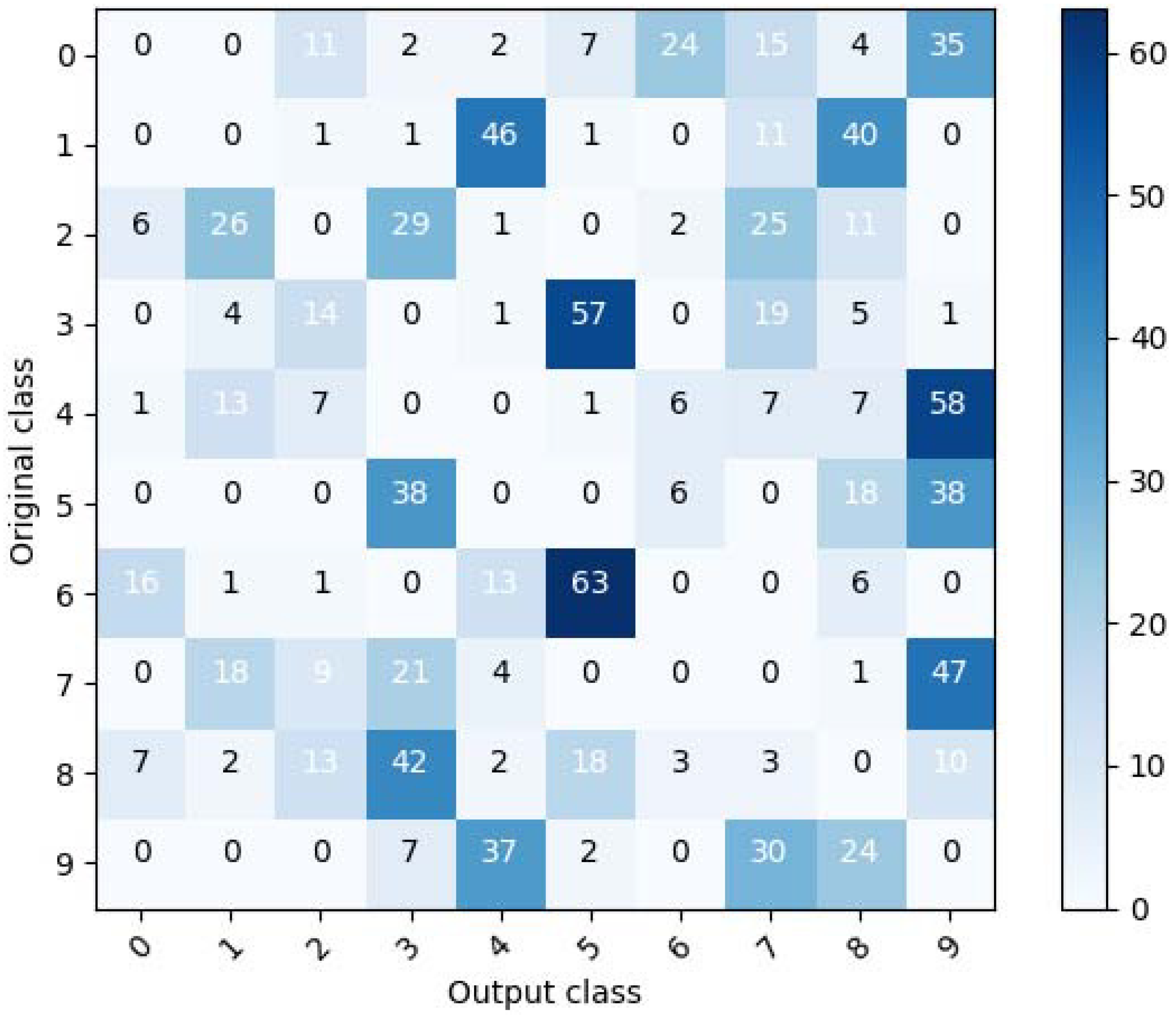
Figure 2 shows the confusion matrix for an untargeted adversarial example for MNIST, the result of testing 100 untargeted adversarial examples for each original class, which were generated using the CW method. As seen in the figure, for a given original class, certain classes have higher numbers than other classes. Therefore, it can be seen that there is a pattern vulnerability. Untargeted adversarial examples concentrate around certain classes for a given original class because it is easier to satisfy misclassification to those classes.
Because a defense system might be able to correctly determine the original class used in generating an untargeted adversarial example by analyzing the pattern’s characteristics, the need may arise to generate an untargeted adversarial example that can overcome this pattern vulnerability. Thus, in this study, we propose the random untargeted adversarial example, which can overcome the pattern vulnerability.
4. Proposed Scheme
4.1. Assumption
The assumption of the proposed method is that the attacker has white-box access to the target model. That is, the attacker knows the target model parameters, architecture, and output classification probabilities. This is a feasible and conservative assumption because a white-box attack can be applied to the case of a black-box model by the construction of a substitute model [11]. By repeating a query process, the method in [11] can be used to generate a substitute network that is similar to the black-box model.
4.2. Proposed Method
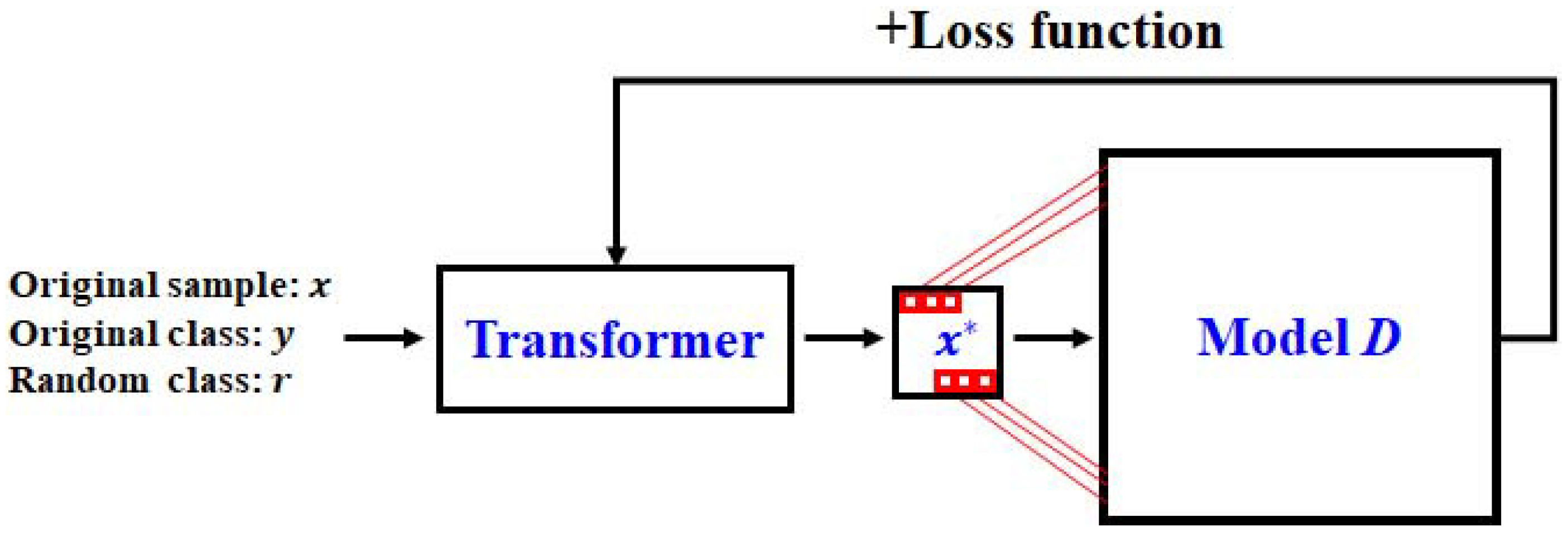
Figure 3 shows the proposed architecture for generating a random untargeted adversarial example. The proposed architecture consists of a transformer and a model D of the classifier. The transformer accepts the original sample x, original class y, and random class r (not the original class) as input values. The transformer then generates a transformer example and provides it to model D. Model D does not change during the generation process. Model D takes the transformed example as an input value and provides the loss function results to the transformer.
The purpose of our architecture is to generate a transformed example that will be misclassified as the random class by model D while minimizing the distance between the transformed example and the original sample x. In the mathematical expressions, the operation function of model D is denoted as . Given the pretrained model D, original sample x, original class y, and random class r (not the original class), we solve the optimization problem to determine a random untargeted adversarial example :
where is the distance between transformed example and original sample x. To achieve the objective that the pretrained model D correctly classify the original sample x as original class y, the following equation is used:
The transformer generates a random untargeted adversarial example by taking the original sample x, original class y, and random class r as the input values. For our study, the transformer presented in [9] was modified as follows:
where is the noise. Model D takes as the input value and outputs the loss function result to the transformer. Then, the transformer calculates the total loss and repeats the above procedure to generate a random untargeted adversarial example while minimizing . This total loss is defined as follows:
where is the distortion of the transformed example, is a classification loss function of D, and c is the weighting value for . The initial value of c is set to 1. is the distance between the transformed example and the original sample x:
To satisfy , must be minimized.
where . Here, r is the random class other than the original class y, and [9,24] indicates the probabilities of the classes being predicted by model D. By optimally minimizing , predicts the probability of the random class to be higher than the probability of the other classes. The procedure for generating the random untargeted adversarial example is given in more detail in Algorithm 1.
| Algorithm 1 Random untargeted adversarial example |
|
5. Experiments and Evaluations
Through experiments, we show that the proposed method can generate a random untargeted adversarial example that will be misclassified as a random class other than the original class by model D while minimizing the distortion distance from the original sample. As the machine learning library, we used TensorFlow [25], and we implemented the method on a Xeon E5-2609 1.7-GHz server.
5.1. Datasets
As datasets in the experiment, MNIST [3] and CIFAR10 [6] were used. MNIST contains handwritten digit images (0∼9) and is a standard dataset. It has the advantages of fast processing time and ease of use in experiments. CIFAR10 contains color images in ten classes: Airplane, car, bird, etc. The MNIST dataset has 60,000 training data and 10,000 test data, and the CIFAR10 dataset has 50,000 training data and 10,000 test data.
5.2. Pretraining of Target Models
The target models pretrained on MNIST and CIFAR10 were common convolutional neural networks (CNNs) [26] and a VGG19 network [27], respectively. Their model architectures and model parameters are shown in Table A1, Table A2 and Table A3 in the Appendix A. For MNIST, 60,000 training data were used to train the target model. In the MNIST test, the pretrained target model [26] correctly recognized the original samples with 99.25% accuracy. In the case of CIFAR10, 50,000 training data were used to train the target model. In the CIFAR10 test, the pretrained target model [27] correctly recognized the original samples with 91.24% accuracy.
5.3. Generation of Test Adversarial Examples
To evaluate the performance of the untargeted adversarial examples, the proposed scheme was used to generate 1000 random untargeted adversarial examples from 1000 random test data. The proposed method is a box constraint method. After narrowing the image range to 0∼1 for each element, the method finds a point causing misclassification through several iterations. In the proposed method, Adam was used as an optimizer of the parameters of the transformer that generates adversarial examples. For MNIST, the learning rate was 0.1, the initial value was 0.001, and the number of iterations was 500. For CIFAR10, the learning rate was 0.01, the initial value was 0.001, and the number of iterations was 6000.
5.4. Experimental Results
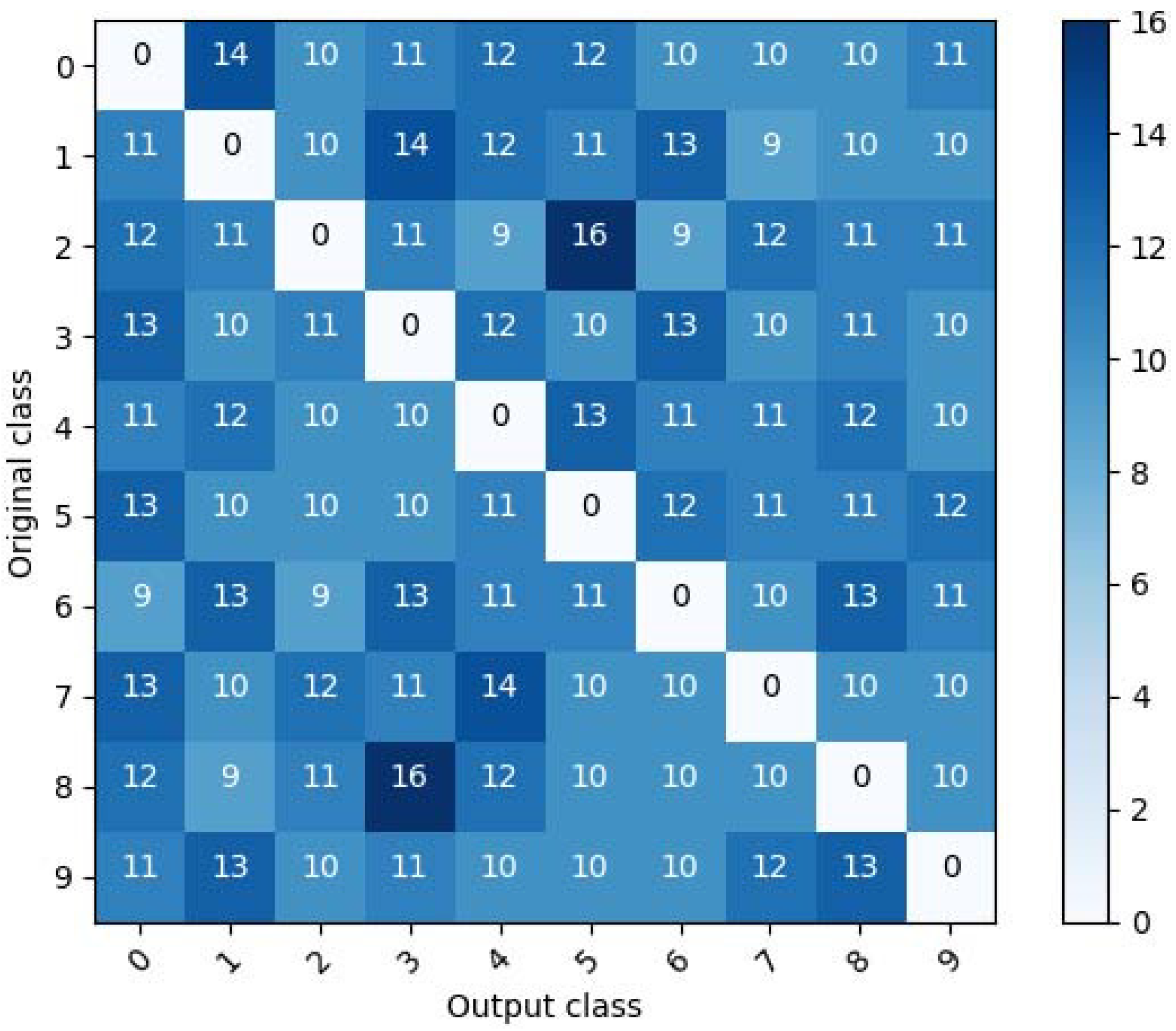
Figure 4 and Figure 5 show the confusion matrix for a random untargeted adversarial example that is classified as a wrong class by the target model D in MNIST and CIFAR10, respectively. In these figures, it is seen that the wrong classes are evenly distributed for each original class. From these results, it can be seen that the proposed scheme eliminates the pattern vulnerability.
Table 1 shows the number of iterations required and the distortion for MNIST and CIFAR10 when the attack success rate of the proposed scheme is 100%. The distortion is defined as the sum of the square root of each pixel’s difference squared (the distance measure). In this table, it is seen that CIFAR10 has more distortion and requires more iterations than MNIST to generate a random untargeted adversarial example. Table 2 shows a sampling of random untargeted adversarial examples that are misclassified by model D when the attack success rate is 100%. To human perception, the random untargeted adversarial examples are similar to their original samples, as shown in Table 2. In addition, Table 3 shows a sampling of random untargeted adversarial examples that are misclassified by model D as each wrong class for original class 1 in MNIST and CIFAR10. In this table, we can see that to the human eye, each adversarial example is similar to the original class 1, although the degree of distortion is different for each image.
Thus, it has been demonstrated that the proposed method can generate a random untargeted adversarial example without pattern vulnerability while maintaining an attack success rate of 100% and human imperception of the change.
5.5. Comparison with the State-of-the-Art Methods
The performance of the proposed method is compared with the state-of-the-art method, CW. Because the CW method is the latest method to improve performance over the known FGSM, I-FGSM, and Deepfool method, this method has 100% attack success and minimal distortion. The CW method can take three forms according to the distortion function used: CW-L, CW-L, and CW-L. “L,” “L,” and “L” refer to the measures of distance between the adversarial example and the original sample, described in Section 2.5.
Table 4 shows untargeted adversarial examples generated on MNIST by the proposed method, the CW-L method, the CW-L method, and the CW-L method. As seen in the table, because the method of applying distortion differs for each method, the image distortion with each method is slightly different. However, with all four methods, the adversarial examples generated are similar to the original sample in terms of human perception. Table 5 shows untargeted adversarial examples generated on CIFAR10 by the proposed method, the CW-L method, the CW-L method, and the CW-L method. In the table, as with Table 4, although distortion is produced differently by each method, it can be seen that it is difficult to detect with the human eye. Unlike MNIST, with CIFAR10 it is difficult to distinguish noise in the color images. Therefore, CIFAR10 is better than MNIST in terms of human perception. The results displayed in Table 4 and Table 5 show that the proposed method has performance similar to that of CW in terms of similarity with the original image for the MNIST and CIFAR10 datasets.
Table 6 shows the average distortion, attack success rate, and presence of pattern vulnerability for the proposed method and the CW-L, CW-L, and CW-L methods. As seen in the table, in terms of average distortion, the proposed scheme produces greater distortion than the CW-L method but less distortion than the other two methods, CW-L and CW-L. However, as seen in Figure 2, Figure 4, and Figure 5, the proposed method has the advantage that it does not have a specific pattern vulnerability, unlike the other three methods.
6. Steganography
The proposed adversarial example can be applied to steganography, as shown in Figure 6. Steganography is a data hiding method by which hidden information is inserted into files, messages, images, and video. Typically, conventional steganography methods insert hidden information using unused bits, frequency transforms, and spatial transforms. Adversarial examples can also be applied to steganography, even though they differ from the conventional steganography methods. By adding small amounts of noise that are not detected by humans, adversarial examples can add hidden information that can only be recognized by the machine. In particular, as the proposed method generates an adversarial example from which a specific pattern is removed, its use in steganography is an improvement over that generated by the use of a conventional untargeted adversarial example.
In order to evaluate the performance of the steganography, we randomly generated 100 adversarial examples using the proposed method with the MNIST and CIFAR10 datasets to test the images on 30 people. Thirty students and researchers from Korea Military Academy and Kongju National University were tested to ascertain the human recognition and detection rates. Figure 7a shows the rates of recognition of 100 original samples and 100 proposed adversarial examples by 30 people. The recognition rate is the proportion of matches between the class identified by human recognition and the original class. The figure shows that the rate of recognition of the proposed adversarial example is similar to the rate of recognition of the original sample. In the case of MNIST, the rate of recognition of the proposed adversarial example is only 2.2% less than the rate of recognition of the original sample. In the case of CIFAR10, the rate of recognition of the proposed adversarial example is almost the same as that of the original sample. For CIFAR10, the rate of recognition of the original sample is about 85% because there is sometimes confusion between a cat and a dog, a deer and a horse, or a car and a truck. Figure 7b shows the rates of detection of 100 original samples and 100 proposed adversarial examples by 30 people. The detection rate is the proportion of matches between the class identified by human detection and the actual class hidden within the image. The detection rate experiment was to ascertain how well a person could detect a hidden image if the proposed adversarial example had a hidden image. As seen in this figure, the detection rate for the proposed adversarial example was similar to random selection (about an 11.1% probability of choosing one of nine classes), because of the low level of distortion from the original sample. In the case of MNIST, as the image is black and white, the distortion is slightly visible to the human eye, and the detection rate is slightly higher than random, by about 3 percentage points. In case of CIFAR10, on the other hand, as the image is three-dimensional, the hidden information is undetected by humans. The above results show that it is possible to apply the proposed method to steganography.
7. Discussion
Attack considerations. The proposed method is useful when an attacker wants to remove pattern vulnerabilities from untargeted adversarial examples. If there is no need to eliminate the pattern vulnerability, a conventional untargeted adversarial example can be used. In military scenarios, however, security issues are more important than system performance because an enemy is being confronted. For this reason, the proposed scheme of generating a random untargeted adversarial example could be used to effectively attack enemy DNNs because it overcomes the pattern vulnerability.
Datasets. We used MNIST and CIFAR10 datasets for our experiments. The MNIST dataset produces less distortion and requires fewer iterations than CIFAR10 because MNIST samples are one-dimensional monochromatic images, and therefore the transformers need fewer generation processes to produce an adversarial example. We have shown that both datasets can be used to generate random untargeted adversarial examples.
The rate of human recognition depends on the characteristics of the dataset. In the case of MNIST, as this dataset consists of numerical images, the recognition rate for the proposed adversarial example is almost 100%. With CIFAR10, however, there can be confusion between a cat and a dog, a deer and a horse, or a car and a truck, so the recognition rates for the proposed adversarial example and the original sample are reduced to 85%. Considering that the CIFAR10 model D accuracy is 91% on CIFAR10, the rate of recognition by the CIFAR10 model D is higher than that by humans.
Distortion. As the distortion rate is the sum of the square roots of each pixel of difference between the adversarial example and the original sample, it is very likely that the distortion will depend on the number of pixels or the dimensionality. For example, each CIFAR10 sample consists of 3072 pixels (32, 32, 3) as a 3D image, and each MNIST sample consists of 784 pixels (28, 28, 1) as a 1D image. Therefore, a CIFAR10 image is more distorted than an MNIST image. However, in the case of CIFAR10, the human eye cannot detect the noise because it is a three-dimensional image. Therefore, the distortion is related to the characteristics of the dataset and is not absolutely proportional to the human recognition rate.
Applications. The proposed method can be applied to road signs. For example, with the use of a random untargeted adversarial example, an enemy vehicle can be caused to misclassify an altered U-turn sign as a random sign that is not a U-turn sign. The proposed scheme can also be applied to steganography. Steganography using the proposed method has the advantage that arbitrary information can be inserted without the weakness of the pattern vulnerability. However, to include information about a particular class, it may be necessary to create a targeted adversarial example to provide information about a particular class.
8. Conclusions
In this study, we proposed the random untargeted adversarial example in order to overcome the pattern vulnerability problem. The proposed method uses an arbitrary class rather than concentrating around specific classes for a given original class when generating an adversarial example. We also presented a steganography application of the proposed scheme. Experimental results show that the proposed method can generate a random untargeted adversarial example without pattern vulnerability while keeping distortion to a minimum (1.99 and 42.32 with MNIST and CIFAR10, respectively) and maintaining a 100% attack success rate. For steganography, the proposed scheme can fool humans, as demonstrated by the probability of their detecting hidden classes being equal to that of random selection. To human perception, the proposed adversarial example is also similar to the original sample. In future research, our experiments will be extended to audio [28] and video domains. A future study will be devoted to developing a defense system for the proposed method.
Author Contributions
H.K. designed the entire architecture and performed the experiments. H.K. wrote the article. Y.K. revised the paper as a whole. D.C. supervised the whole process as a corresponding author. Y.K., H.Y. and D.C. gave some advice and ideas about the article. All authors analyzed the result of this article. All authors discussed the contents of the manuscript.
Acknowledgments
This study was supported by the Institute for Information & Communications Technology Promotion (Grant No. 2016-0-00173) and the National Research Foundation (Grant No. 2017R1A2B4006026 and 2016R1A4A1011761).
Conflicts of Interest
The authors declare no conflict of interest.
Appendix A

Table A1.
Target model architecture for MNIST; “Conv.” is a convolution.
| Type of Layer | Shape |
|---|---|
| Conv. + ReLU | [3, 3, 32] |
| Conv. + ReLU | [3, 3, 32] |
| Max pooling | [2, 2] |
| Conv. + ReLU | [3, 3, 64] |
| Conv. + ReLU | [3, 3, 64] |
| Max pooling | [2, 2] |
| Fully connected + ReLU | [200] |
| Fully connected + ReLU | [200] |
| Softmax | [10] |
Table A2.
Target model specifications.
| Item | MNIST | CIFAR10 |
|---|---|---|
| Learning rate | 0.1 | 0.1 |
| Momentum | 0.9 | 0.9 |
| Delay rate | - | 10 (decay 0.0001) |
| Dropout | 0.5 | 0.5 |
| Batch size | 128 | 128 |
| Epochs | 50 | 200 |
Table A3.
Target model architecture [27] for CIFAR10; “Conv.” is a convolution.
Table A3.
Target model architecture [27] for CIFAR10; “Conv.” is a convolution.
| Type of Layer | Shape |
|---|---|
| Conv. + ReLU | [3, 3, 64] |
| Conv. + ReLU | [3, 3, 64] |
| Max pooling | [2, 2] |
| Conv. + ReLU | [3, 3, 128] |
| Conv. + ReLU | [3, 3, 128] |
| Max pooling | [2, 2] |
| Conv. + ReLU | [3, 3, 256] |
| Conv. + ReLU | [3, 3, 256] |
| Conv. + ReLU | [3, 3, 256] |
| Conv. + ReLU | [3, 3, 256] |
| Max pooling | [2, 2] |
| Conv. + ReLU | [3, 3, 512] |
| Conv. + ReLU | [3, 3, 512] |
| Conv. + ReLU | [3, 3, 512] |
| Conv. + ReLU | [3, 3, 512] |
| Max pooling | [2, 2] |
| Conv. + ReLU | [3, 3, 512] |
| Conv. + ReLU | [3, 3, 512] |
| Conv. + ReLU | [3, 3, 512] |
| Conv. + ReLU | [3, 3, 512] |
| Max pooling | [2, 2] |
| Fully connected + ReLU | [4096] |
| Fully connected + ReLU | [4096] |
| Softmax | [10] |
References
- Schmidhuber, J. Deep learning in neural networks: An overview. Neural Netw. 2015, 61, 85–117. [Google Scholar] [CrossRef] [PubMed] [Green Version]
- Szegedy, C.; Zaremba, W.; Sutskever, I.; Bruna, J.; Erhan, D.; Goodfellow, I.; Fergus, R. Intriguing properties of neural networks. In Proceedings of the International Conference on Learning Representations, Banff, AB, Canada, 14–16 April 2014. [Google Scholar]
- LeCun, Y.; Cortes, C.; Burges, C.J. MNIST Handwritten Digit Database. AT&T Labs. 2010, Volume 2. Available online: http://yann.lecun.com/exdb/mnist (accessed on 4 December 2018 ).
- Kwon, H.; Kim, Y.; Yoon, H.; Choi, D. Fooling a Neural Network in Military Environments: Random Untargeted Adversarial Example. In Proceedings of the Military Communications Conference, Los Angeles, CA, USA, 29–31 October 2018. [Google Scholar]
- Cheddad, A.; Condell, J.; Curran, K.; Mc Kevitt, P. Digital image steganography: Survey and analysis of current methods. Signal Process. 2010, 90, 727–752. [Google Scholar] [CrossRef] [Green Version]
- Krizhevsky, A.; Nair, V.; Hinton, G. The CIFAR-10 Dataset. 2014. Available online: http://www.cs.toronto.edu/kriz/cifar.html (accessed on 4 December 2018 ).
- Barreno, M.; Nelson, B.; Joseph, A.D.; Tygar, J. The security of machine learning. Mach. Learn. 2010, 81, 121–148. [Google Scholar] [CrossRef] [Green Version]
- Biggio, B.; Nelson, B.; Laskov, P. Poisoning attacks against support vector machines. In Proceedings of the 29th International Coference on International Conference on Machine Learning, Edinburgh, UK, 26 June–1 July 2012; pp. 1467–1474. [Google Scholar]
- Carlini, N.; Wagner, D. Towards evaluating the robustness of neural networks. In Proceedings of the 2017 IEEE Symposium on Security and Privacy (SP), San Jose, CA, USA, 22–24 May 2017; pp. 39–57. [Google Scholar]
- Moosavi-Dezfooli, S.M.; Fawzi, A.; Frossard, P. Deepfool: A simple and accurate method to fool deep neural networks. In Proceedings of the IEEE Conference on Computer Vision and Pattern Recognition, Las Vegas, NV, USA, 26 June–1 July 2016; pp. 2574–2582. [Google Scholar]
- Papernot, N.; McDaniel, P.; Goodfellow, I.; Jha, S.; Celik, Z.B.; Swami, A. Practical black-box attacks against machine learning. In Proceedings of the 2017 ACM on Asia Conference on Computer and Communications Security, Abu Dhabi, UAE, 2–6 April 2017; pp. 506–519. [Google Scholar]
- Kwon, H.; Kim, Y.; Park, K.W.; Yoon, H.; Choi, D. Advanced Ensemble Adversarial Example on Unknown Deep Neural Network Classifiers. IEICE Trans. Inf. Syst. 2018, 101, 2485–2500. [Google Scholar] [CrossRef]
- Meng, D.; Chen, H. Magnet: A two-pronged defense against adversarial examples. In Proceedings of the 2017 ACM SIGSAC Conference on Computer and Communications Security, Dallas, TX, USA, 30 October–3 November 2017; pp. 135–147. [Google Scholar]
- Carlini, N.; Wagner, D. Adversarial examples are not easily detected: Bypassing ten detection methods. In Proceedings of the 10th ACM Workshop on Artificial Intelligence and Security, Dallas, TX, USA, 3 November 2017; pp. 3–14. [Google Scholar]
- Kwon, H.; Yoon, H.; Choi, D. POSTER: Zero-Day Evasion Attack Analysis on Race between Attack and Defense. In Proceedings of the 2018 on Asia Conference on Computer and Communications Security, Songdo, Incheon, Korea, 4–8 June 2018; pp. 805–807. [Google Scholar]
- Kurakin, A.; Goodfellow, I.J.; Bengio, S. Adversarial Machine Learning at Scale. In Proceedings of the International Conference on Learning Representations (ICLR), Toulon, France, 24–26 April 2017. [Google Scholar]
- Narodytska, N.; Kasiviswanathan, S. Simple black-box adversarial attacks on deep neural networks. In Proceedings of the 2017 IEEE Conference on Computer Vision and Pattern Recognition Workshops (CVPRW), Honolulu, HI, USA, 21–26 July 2017; pp. 1310–1318. [Google Scholar]
- Strauss, T.; Hanselmann, M.; Junginger, A.; Ulmer, H. Ensemble Methods as a Defense to Adversarial Perturbations Against Deep Neural Networks. arXiv, 2017; arXiv:1709.03423. [Google Scholar]
- Goodfellow, I.; Shlens, J.; Szegedy, C. Explaining and Harnessing Adversarial Examples. In Proceedings of the International Conference on Learning Representations, San Diego, CA, USA, 7–9 May 2015. [Google Scholar]
- Kurakin, A.; Goodfellow, I.; Bengio, S. Adversarial examples in the physical world. In Proceedings of the ICLR Workshop, Toulon, France, 24–26 April 2017. [Google Scholar]
- Papernot, N.; McDaniel, P.; Wu, X.; Jha, S.; Swami, A. Distillation as a defense to adversarial perturbations against deep neural networks. In Proceedings of the 2016 IEEE Symposium on Security and Privacy (SP), San Jose, CA, USA, 23–25 May 2016; pp. 582–597. [Google Scholar]
- Kwon, H.; Kim, Y.; Park, K.W.; Yoon, H.; Choi, D. Friend-safe Evasion Attack: An adversarial example that is correctly recognized by a friendly classifier. Comput. Secur. 2018, 78, 380–397. [Google Scholar] [CrossRef]
- Kwon, H.; Kim, Y.; Park, K.W.; Yoon, H.; Choi, D. Multi-Targeted Adversarial Example in Evasion Attack on Deep Neural Network. IEEE Access 2018, 6, 46084–46096. [Google Scholar] [CrossRef]
- Papernot, N.; McDaniel, P.; Jha, S.; Fredrikson, M.; Celik, Z.B.; Swami, A. The limitations of deep learning in adversarial settings. In Proceedings of the 2016 IEEE European Symposium on Security and Privacy, San Jose, CA, USA, 23–25 May 2016; pp. 372–387. [Google Scholar]
- Abadi, M.; Barham, P.; Chen, J.; Chen, Z.; Davis, A.; Dean, J.; Devin, M.; Ghemawat, S.; Irving, G.; Isard, M.; et al. TensorFlow: A System for Large-Scale Machine Learning. In Proceedings of the 12th USENIX Symposium on Operating Systems Design and Implementation, Savannah, GA, USA, 2–4 November 2016; Volume 16, pp. 265–283. [Google Scholar]
- LeCun, Y.; Bottou, L.; Bengio, Y.; Haffner, P. Gradient-based learning applied to document recognition. Proc. IEEE 1998, 86, 2278–2324. [Google Scholar] [CrossRef] [Green Version]
- He, K.; Zhang, X.; Ren, S.; Sun, J. Deep residual learning for image recognition. In Proceedings of the IEEE Conference on Computer Vision and Pattern Recognition, Las Vegas, NV, USA, 27–30 June 2016; pp. 770–778. [Google Scholar]
- Kereliuk, C.; Sturm, B.L.; Larsen, J. Deep learning and music adversaries. IEEE Trans. Multimed. 2015, 17, 2059–2071. [Google Scholar] [CrossRef]
Figure 1.
Architecture of a neural network.
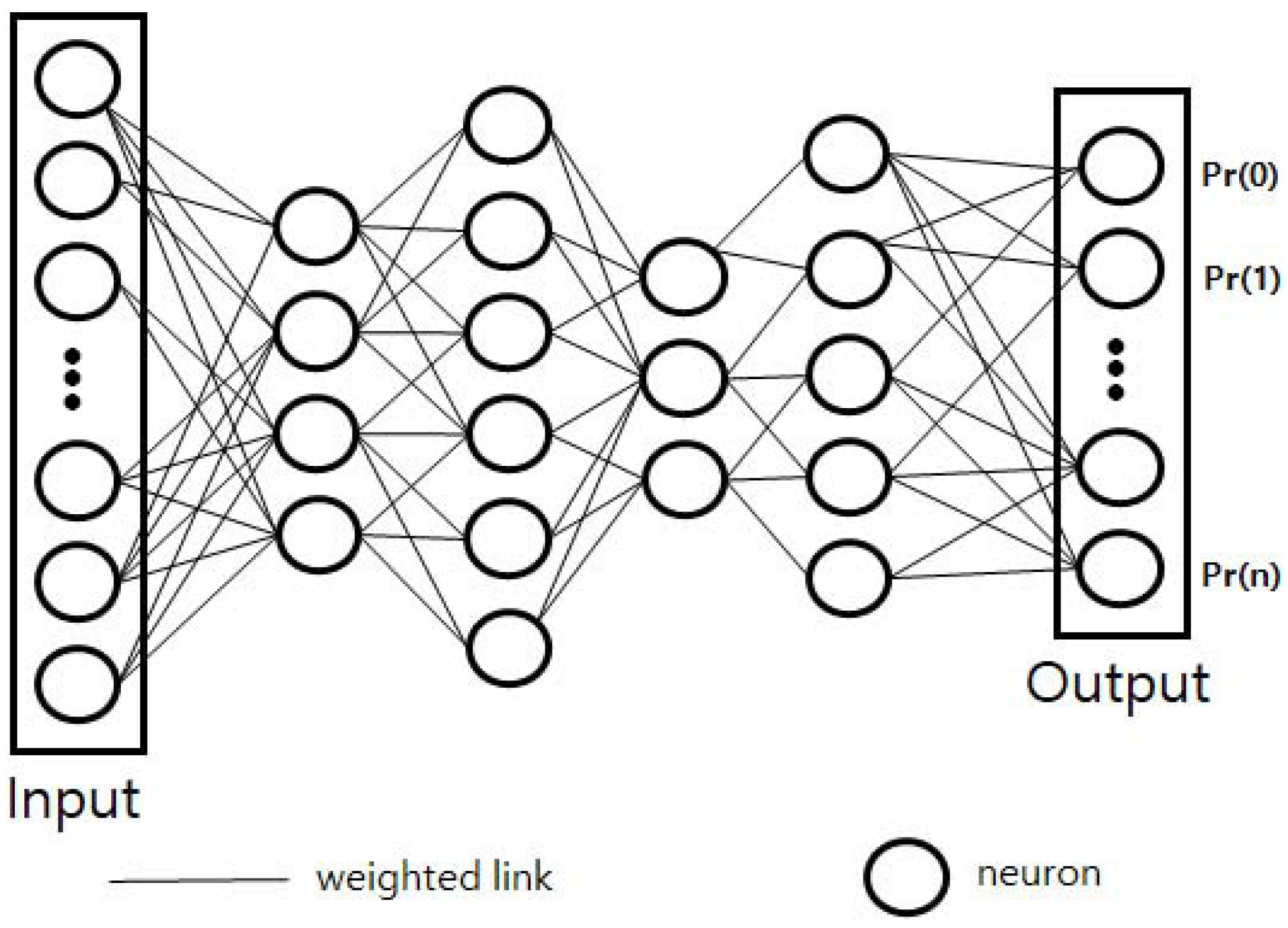
Figure 2.
Confusion matrix for an untargeted adversarial example in MNIST [3].
Figure 2.
Confusion matrix for an untargeted adversarial example in MNIST [3].

Figure 3.
Proposed architecture.

Figure 4.
Confusion matrix of a target model for a random untargeted class in MNIST.
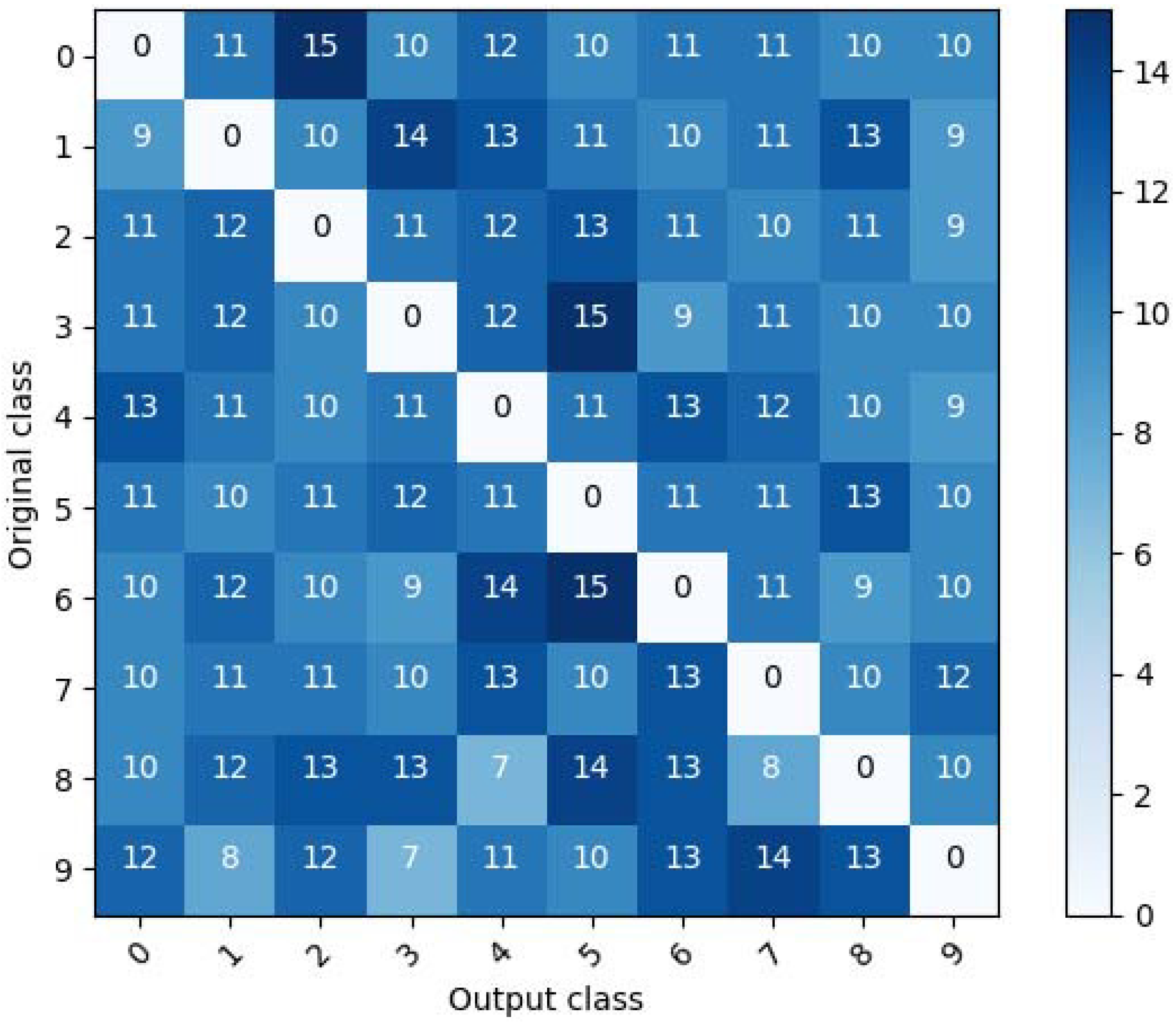
Figure 5.
Confusion matrix of a target model for a random untargeted class in CIFAR10: “0-airplanes,” “1-cars,” “2-birds,” “3-cats,” “4-deer,” “5-dogs,” “6-frogs,” “7-horses,” “8-ships,” and “9-trucks.”
Figure 5.
Confusion matrix of a target model for a random untargeted class in CIFAR10: “0-airplanes,” “1-cars,” “2-birds,” “3-cats,” “4-deer,” “5-dogs,” “6-frogs,” “7-horses,” “8-ships,” and “9-trucks.”

Figure 6.
Steganography scheme using the proposed adversarial example.

Figure 7.
Average recognition and detection rates for the random untargeted adversarial example in human testing.
Figure 7.
Average recognition and detection rates for the random untargeted adversarial example in human testing.
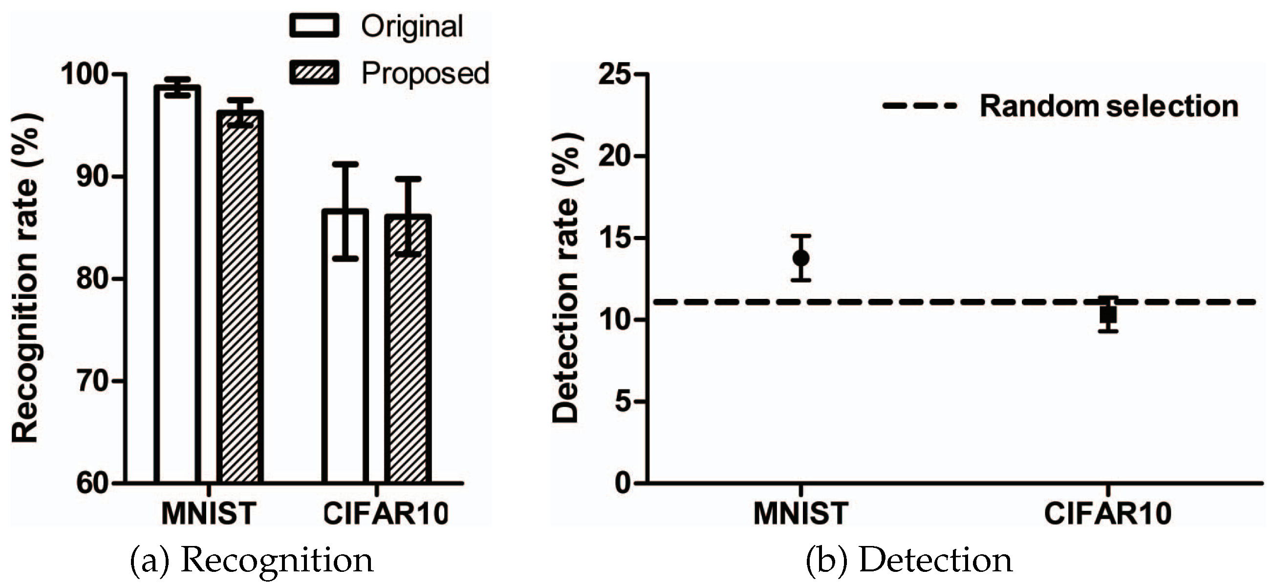
Table 1.
Comparison of MNIST and CIFAR10 with 100% attack success. SD is standard deviation.
| Characteristic | MNIST | CIFAR10 |
|---|---|---|
| Number of iterations | 500 | 6000 |
| Maximum distortion | 5.494 | 177.4 |
| Minimum distortion | 0.025 | 0.004 |
| SD of distortion | 0.713 | 24.580 |
| Mean distortion | 1.99 | 42.324 |
Table 2.
Sampling of random untargeted adversarial examples. CIFAR10 has “0-airplanes,” “1-cars,” “2-birds,” “3-cats,” “4-deer,” “5-dogs,” “6-frogs,” “7-horses,” “8-ships,” and “9-trucks.”
Table 2.
Sampling of random untargeted adversarial examples. CIFAR10 has “0-airplanes,” “1-cars,” “2-birds,” “3-cats,” “4-deer,” “5-dogs,” “6-frogs,” “7-horses,” “8-ships,” and “9-trucks.”
| Wrong Class | 0 | 1 | 2 | 3 | 4 | 5 | 6 | 7 | 8 | 9 |
|---|---|---|---|---|---|---|---|---|---|---|
| MNIST |  |  |  |  |  |  |  |  |  |  |
 |  |  |  |  |  |  |  |  |  | |
 |  |  |  |  |  |  |  |  |  | |
| CIFAR10 |  |  |  |  |  |  |  |  |  |  |
 |  |  |  |  |  |  |  |  |  | |
 |  |  |  |  |  |  |  |  |  |
Table 3.
Sampling of random untargeted adversarial examples in class 1. CIFAR10 has “0-airplanes,” “1-cars,” “2-birds,” “3-cats,” “4-deer,” “5-dogs,” “6-frogs,” “7-horses,” “8-ships,” and “9-trucks.”
Table 3.
Sampling of random untargeted adversarial examples in class 1. CIFAR10 has “0-airplanes,” “1-cars,” “2-birds,” “3-cats,” “4-deer,” “5-dogs,” “6-frogs,” “7-horses,” “8-ships,” and “9-trucks.”
| Wrong Class | 0 | 2 | 3 | 4 | 5 | 6 | 7 | 8 | 9 |
|---|---|---|---|---|---|---|---|---|---|
| MNIST |  |  |  |  |  |  |  |  |  |
| CIFAR10 |  |  |  |  |  |  |  |  |  |
Table 4.
A sampling of the untargeted adversarial examples generated on MNIST by the proposed method, the CW-L method, the CW-L method, and the CW-L method.
Table 4.
A sampling of the untargeted adversarial examples generated on MNIST by the proposed method, the CW-L method, the CW-L method, and the CW-L method.
| Original |  |  |  |  |  |  |  |  |  |  |
| Proposed |  |  |  |  |  |  | |  |  |  |
| CW-L |  |  |  |  |  |  |  |  |  |  |
| CW-L |  |  |  |  |  |  |  |  |  |  |
| CW-L |  |  |  |  |  |  |  |  |  |  |
Table 5.
A sampling of the untargeted adversarial examples generated on CIFAR10 by the proposed method, the CW-L method, the CW-L method, and the CW-L method.
Table 5.
A sampling of the untargeted adversarial examples generated on CIFAR10 by the proposed method, the CW-L method, the CW-L method, and the CW-L method.
| Original |  |  |  |  |  |  |  |  |  |  |
| Proposed |  |  |  |  |  |  |  |  |  |  |
| CW-L |  |  |  |  |  |  |  |  |  |  |
| CW-L |  |  |  |  |  |  |  |  |  |  |
| CW-L |  |  |  |  |  |  |  |  |  |  |
Table 6.
Comparison of the proposed scheme, CW-L method, CW-L method, and CW-L method.
| Characteristic | MNIST | CIFAR10 | ||||||
|---|---|---|---|---|---|---|---|---|
| Proposed | CW-L | CW-L | CW-L | Proposed | CW-L | CW-L | CW-L | |
| Average distortion | 1.99 | 2.51 | 1.40 | 2.16 | 42.32 | 49.92 | 27.41 | 47.21 |
| Attack success rate | 100% | 100% | 100% | 100% | 100% | 100% | 100% | 100% |
| Pattern vulnerability? | No | Yes | Yes | Yes | No | Yes | Yes | Yes |
© 2018 by the authors. Licensee MDPI, Basel, Switzerland. This article is an open access article distributed under the terms and conditions of the Creative Commons Attribution (CC BY) license (http://creativecommons.org/licenses/by/4.0/).
Share and Cite
MDPI and ACS Style
Kwon, H.; Kim, Y.; Yoon, H.; Choi, D. Random Untargeted Adversarial Example on Deep Neural Network. Symmetry 2018, 10, 738. https://0-doi-org.brum.beds.ac.uk/10.3390/sym10120738
AMA Style
Kwon H, Kim Y, Yoon H, Choi D. Random Untargeted Adversarial Example on Deep Neural Network. Symmetry. 2018; 10(12):738. https://0-doi-org.brum.beds.ac.uk/10.3390/sym10120738
Chicago/Turabian StyleKwon, Hyun, Yongchul Kim, Hyunsoo Yoon, and Daeseon Choi. 2018. "Random Untargeted Adversarial Example on Deep Neural Network" Symmetry 10, no. 12: 738. https://0-doi-org.brum.beds.ac.uk/10.3390/sym10120738
Note that from the first issue of 2016, this journal uses article numbers instead of page numbers. See further details here.