Localized Fault Tolerant Algorithm Based on Node Movement Freedom Degree in Flying Ad Hoc Networks

College of Information and Communication Engineering, Harbin Engineering University, Harbin 150001, China
*
Author to whom correspondence should be addressed.
Symmetry 2019, 11(1), 106; https://0-doi-org.brum.beds.ac.uk/10.3390/sym11010106
Submission received: 12 December 2018
/
Revised: 11 January 2019
/
Accepted: 13 January 2019
/
Published: 17 January 2019
Abstract
:Flying ad hoc network (FANET) is a communication network for data transmission among Unmanned Aerial Vehicles (UAVs). In ad hoc network, the UAVs movement is usually applied to improve network fault-tolerance, but it easily causes the disconnection of communication links, and the success rate is low. In this paper, we propose a local fault-tolerant control algorithm based on node movement freedom degree (LFTMF). Under the constraint of node movement freedom degree, the algorithm transforms the single-connected network into bi-connected network through the autonomous movement of UAVs to improve the fault-tolerant ability of the FANET network. Firstly, the consistency between k-hop cut-points and global cut-points in FANET network is analyzed. Then, based on the k-hop local topology of FANET network, the UAV node movement freedom degree model is established. Finally, according to the location distribution of k-hop cut-points in the FANET network, the bi-connected fault-tolerant network is realized by UAVs cascade movement. Compared with the existing algorithms, simulation results show that the proposed algorithm achieves better performance in success rate, deviation distance, cascade movement ratio and adjustment period.
1. Introduction
Unmanned Aerial Vehicles (UAVs) cluster intelligence and cooperation depend on timely and effective information exchange between different nodes, therefore the communication network is one of the most important design issues of multi-UAV system [1]. UAVs exchange data or instructions through one or more hops in FANET, which is a center-free ad hoc network between UAVs [2]. In three-dimensional single-connected FANET networks, the movement or failure of some UAVs will lead to the disconnection of communication links or network partition, resulting in data transmission failure [3,4,5]. Therefore, it is an urgent problem to establish fault-tolerant networks to ensure the reliable end-to-end connection between UAVs.
A network is defined as bi-connected if there are two disjoint communication paths between any pair of UAV nodes in the network, which is the basic goal of the FANET network fault-tolerant design [6]. Topology control is an effective method to realize fault-tolerant networks [7], which can be divided into three categories. The first method is to maintain network connectivity by adjusting the transmit power of nodes in the network [8,9]. Fidel Aznar [10] proposed a theoretical model of the swarm energy consumption to describe the UAVs energy consumed. R. Ramanathan [11] proposed two distributed heuristic algorithms, which adaptively adjust the transmit power of nodes according to the topology changes and attempts to maintain the topology connectivity using the minimum power. In [12], an adaptive topology control algorithm is proposed to improve the network performance by controlling the transmit power to change the transmission range. M. Mozaffari [13] and F. Lagum [14] analyzed the deployment of a UAV as a flying base station and minimized the total required transmit power of UAV while covering the entire area. However, sometimes the distance between UAVs is so long that the maximum transmit power may be unable to achieve connectivity. The second method is to add relay nodes to the network to improve the fault tolerance capability of UAV network [15,16]. Kashyap A [17] reconstructed the topology of ad hoc network by adding relay nodes to meet the fault tolerance requirements of the network. Jie LI [18] proposed maintaining the fault tolerance UAV ad hoc network through the speed control of relay nodes. However, the additional relay nodes increase the UAV quantity cost. The third method is to use UAV movement in cluster to achieve bi-connected fault-tolerant network [19]. Prithwish first proposed the centralized block movement algorithm [20], but the global topology information of UAV cluster is difficult to obtain and the distance of deviation from original track is too long. Shantanu proposed the distributed node movement algorithm to implement a bi-connected fault-tolerant network [21], but the algorithm causes the disconnection of the original communication link, and the recovery success rate in the sparse network is not high. UAV moves in three-dimensional space, but the existing research on mobile topology control is based on two-dimensional space [19,20,21,22]. Therefore, the research of distributed movement control based on three-dimensional space is of great significance to improve the fault tolerance of UAV dynamic network.
To realize fault-tolerant network, we adopt local movement management to control the network topology. As every UAV has its own task, we can only change its movement in a limited range and direction, which is challenging work. In this paper, we propose the localized fault-tolerant algorithm based on node movement freedom degree (LFTMF) for single-connected FANET networks to realize fault-tolerant network with minimum movement cost. The main contributions are as follows. Firstly, the movement freedom degree model of UAV nodes is established based on k-hop local topology of UAV nodes in three-dimensional FANET. Then, we analyze the consistency of k-hop cut points and global cut points. Finally, we adopt local cascade movement management to achieve bi-connected fault tolerant networks.
2. Model and Problem Analysis
The signal transmission in space will cause the change of the receiving power, which will decrease with the increase of the distance between the transmission node and the receiving node. This phenomenon is called large-scale fading model, which is the most basic channel model for FANET network research. When a UAV node sends a wireless signal to in FANET, the receiving power of UAV node j is shown in Equation (1).
Equation (1) is Fries transfer formula, where is the transmission power of node , and is the carrier wavelength of the wireless signal. is the distance between the transmission node and the receiving node . is the path loss coefficient and the worse the environment, the greater the value. is the antenna gain of the transmission node and is the antenna gain of the receiving node. is the loss factor.
In free space, the value of power of noise and interference is assumed to be constant. is the threshold of SNR. Then, the receiving power satisfies Equation (2).
When , , and , the maximum transmission distance is shown as Equation (3).
The paper assumes that the transmitters are the same and the receivers are the same in FANET network. The values of , and are constant. Then, the definition of constant C is shown as Equation (4).
From Equation (5), it can be seen that the maximum transmission distance is proportional to the powers of transmission power . Given the value of transmission power, the value of the maximum transmission distance of the signal is unique. Therefore, we use the distance to represent transmission power in the latter sections.
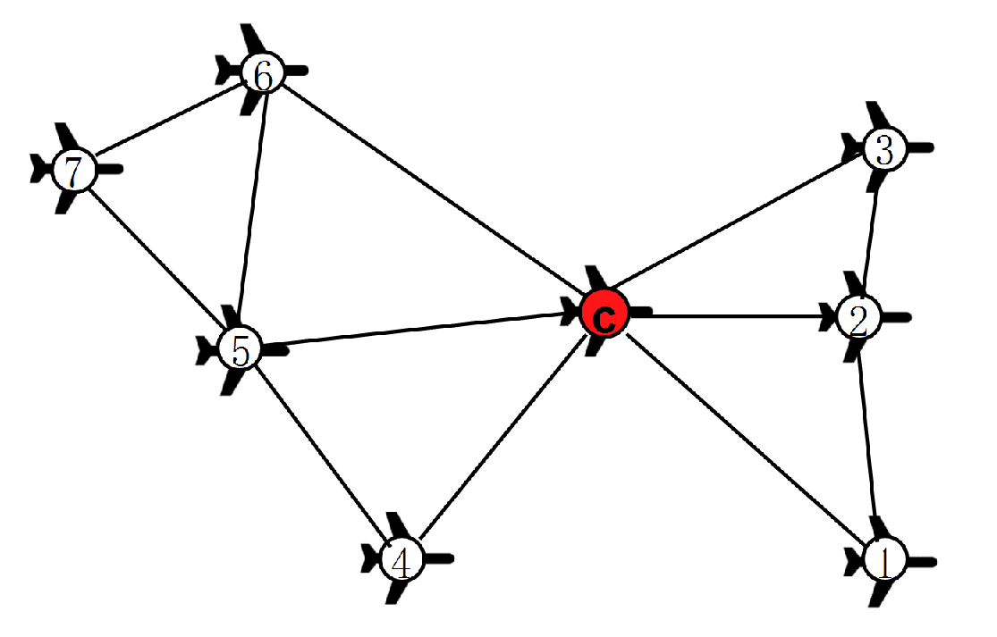
UAV cluster carries out reconnaissance tasks in three-dimensional barrier-free space, flying in a straight line and every UAV is equipped with GPS and a wireless transceiver with communication distance . If the distance between two UAVs is not greater than , the two UAV nodes are neighbors and have bi-way communication links. This paper assumes that FANET is an isomorphic network. Nodes corresponds to UAVs and the bi-way communication links between nodes is represented as edges . UAV nodes and communication links constitute three-dimensional FANET networks topology graph , and the network topology schematic diagram is shown in Figure 1. As the network topology only represents the relative position relationship between UAVs, the topology is planform of three-dimensional network topology in this paper.
At the initial time, the FANET network is single connected, but it is prone to be partitioned, which leads to the failure of communication links. Therefore, it is necessary to construct fault-tolerant network and minimize the distance of deviation from original track.
2.1. Node Movement Freedom Degree Model
To better describe the node movement freedom degree model, some symbols and their definitions are shown in Table 1.
Some important definitions are as follows.
Definition 1.
k-hop local topology, also known as k-hop derived subgraph. Suppose is a node in the network topology graph G and is the derived subgraph of G. If all the nodes in are composed of and its k-hop neighbors, then G is the k-hop local topology of of G.
Definition 2.
k-hop cut point. In the network topology graph G, if c is the cut point of its k-hop local topology, then c is the k-hop cut point.
Definition 3.
Network node density, also called average node degree. The ratio value of the node degree of all nodes in the network topology graph G to the total number of nodes in G is the network node density.
Definition 4.
Generalized leaf nodes. Nodes with a node degree of 1 in the network topology graph G are called leaf nodes. For a cut point c, there exists a set , and the neighbor nodes of any node in set A satisfy condition , then the nodes in set A are called generalized leaf nodes.
In the k-hop topology of cut point c, the the movement freedom degree of node on direction is defined as the maximum distance that node could move while maintaining connectivity with all its neighbors in direction . That is to say, the minimum value of the maximum distance of deviation from original track on direction on the premise that node is connected to each neighbor node , and the details are shown in Equation (6).
where is the maximum distance matrix of deviation from original track of node on direction , constrained by its neighbor node . Element in denotes the maximum movement distance of node on direction only under the constraint of its neighbor . According to cosine theorem, satisfies Equation (7).
where represents the angle between vector and vector and represents the set of kth-hop neighbor nodes of cut point c. The conditions under which Equation (7) has a feasible solution are shown as the inequality in Equation (8).
The inequality in Equation (8) is always established. Thus, the solution of Equation (7) is shown in Equation (9), and the derivation process is as follows.
Because ,
2.2. Problem Analysis
To describe the problem more conveniently, some of the theorems are as follows.
Theorem 1.
If the network is bi-connected, there are no global cut-points in the network topology. If there are no global cut-points in the network topology, the network is bi-connected at least, which means that the network has bi-connectivity or higher connectivity.
Proof of Theorem 1.
Firstly, if the network topology graph G satisfies bi-connectivity, there will be at least two disjoint communication paths between any pair of nodes and in the graph G. Assuming that there is a global cut-point c in the topology graph of a bi-connected network G and a pair nodes . After removing node c, there is no communication path between and , which is in contradiction with that G satisfies bi-connectivity. Therefore, if the network topology graph G satisfies bi-connectivity, there is no global cut-point in the G. Then, if the network topology graph G does not have global cut-points, removing any node will not lead to network partition. Therefore, G is not single-connected and it is bi-connected at least. □
A network topology graph G is defined as k-connected if there are k disjoint communication paths between any pair of UAV nodes in the network. When , the network topology G is single connected and when , the network topology G has fault-tolerant ability and good invulnerability. Therefore, is set to construct a bi-connected fault-tolerant network in this paper. According to Theorem 1, the construction of bi-connected fault-tolerant network can be transformed into the problem of changing cut-points into non-cut points in the network. As the global topology information is unknown, it is necessary to study the cut-point detection algorithm based on k-hop local topology, and approximately minimize the node offset distance based on k-hop local topology of cut-points. The offset distance is the distance of deviation from original track of UAV in this paper.
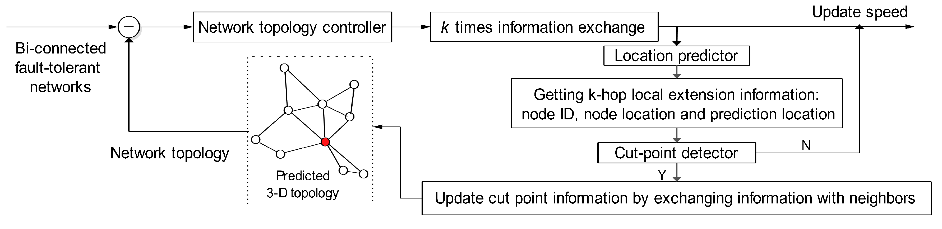
FANET network fault-tolerant control problem is abstracted as the closed-loop control model shown in Figure 2, and the red node in the predicted topology is cut-point.
The initial network topology is single connected and every UAV executes the control flow.
Step 1: The location of every UAV in the cluster is at time t, and the location predictor of predicts its location of time . The k-hop local topology information, which contains the ID of each node and the location information of every UAV at time t and time , is obtained by k times information exchange with its neighbors. According to the location relationship of nodes, we could get the k-hop local topology of time t and the k-hop local topology of time .
Step 2: The cut-point detector on executes the cut-point detection algorithm based on to determine whether itself is a cut-point. If is a cut-point, update the cut-point information of the k-hop local topology and then obtain by once information exchange with its neighbors.
Step 3: The topology controller of node recalculates the location of UAV nodes in the k-hop local topology of time according to the network fault-tolerance requirements and the predicted local network topology . Then, the movement instructions are sent to the destination UAV node through k times information exchange. Finally, the destination UAV node updates its speed according to the decision rules.
3. The Construction of Bi-Connected Fault-Tolerant Networks
3.1. Cut-Point Detection Algorithm Based on k-Hop Local Topology Information
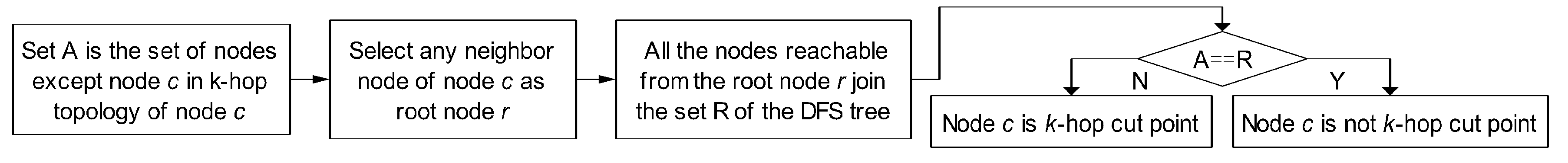
It is the premise of the construction of bi-connected fault-tolerant network to analyze the consistency between k-hop cut-point and global cut-point. Therefore, we study cut-point detection algorithm based on k-hop local topology information. UAV node c can obtain its k-hop local topology by k times information exchange with its neighbors. Then, the depth first search (DFS) algorithm is used to determine whether it is a k-hop cut-point. The flow chart of the algorithm is shown in Figure 3.
3.2. Localized Fault-Tolerant Algorithm Based on Node Movement Freedom Degree (LFTMF)
There are two methods to control node movement: block movement and cascade movement [19]. Block movement is that all UAV nodes in a connected block participate in the movement, which would have a bad impact on the original task. The cascade movement is that some nodes participate in the movement, while others move in the original direction. Therefore, cascade motion is adopted to realize bi-connected fault-tolerant network.
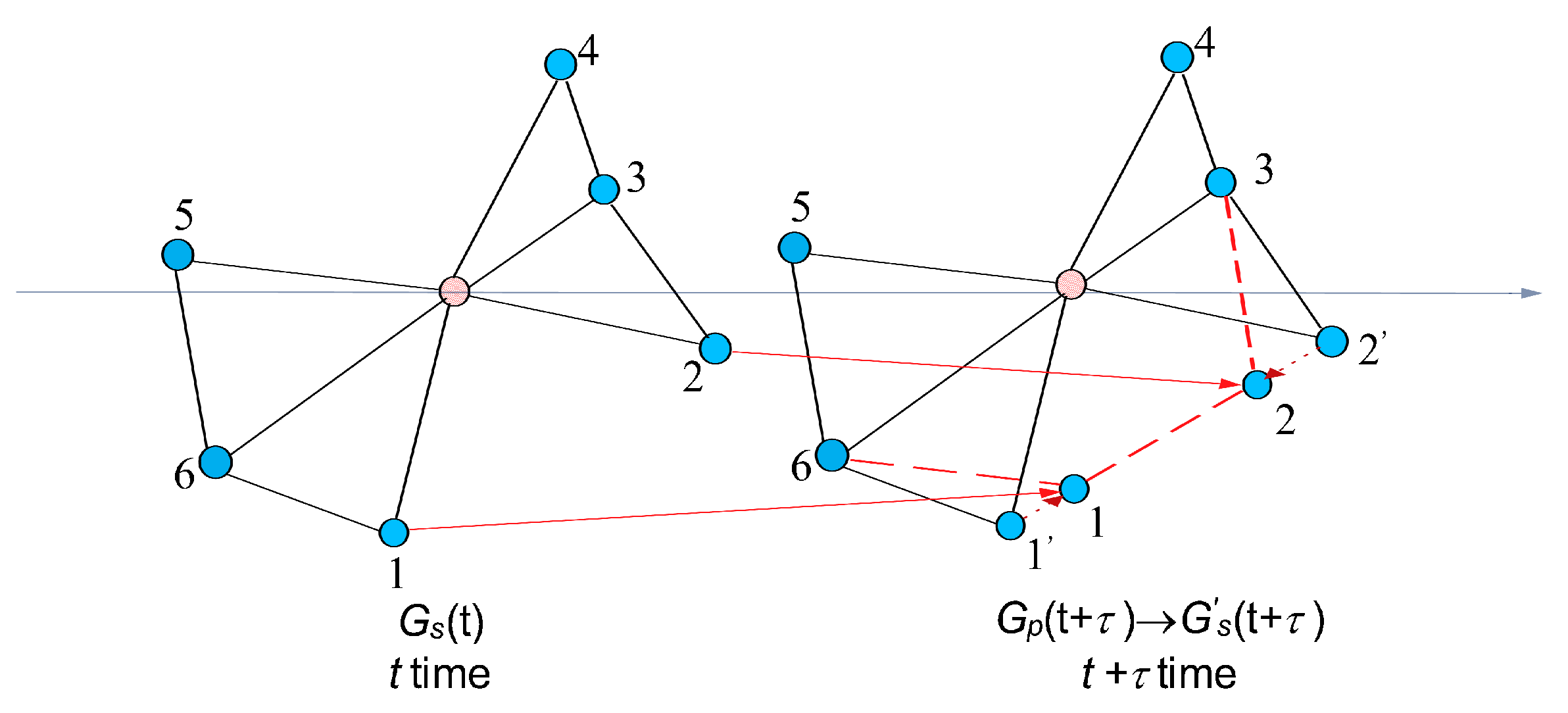
As shown in Figure 4, at time t, the k-hop local topology of a cut-point c is where the node c is a cut-point. The predicted location of UAV nodes at time is , which corresponds to the predicted k-hop local topology graph , consisting of nodes and black solid lines among them of time . Based on , the locations of node and node a are moved to node 1 and node 2, respectively. Then, the location at time is temporarily updated to , as shown in Equation (10), which corresponds to the k-hop local topology graph , consisting of nodes and black solid lines or red dashed lines among them at time .
where predicted by location predictor is the location of node at time . is the offset vector of node and corresponds to the red dashed arrows which from node to node 1 and from node to node 2 in Figure 4. All location points are three-dimensional. is the movement freedom degree of node in the direction . The total offset distance based on the k-hop local topology of the cut-point c is shown in Equation (11). The objective of optimization is to minimize , while guaranteeing the realization of bi-connected fault-tolerant networks.
The decision rules for directive execution are as follows. Since a node may exists in the k-hop local topology of different cut-points, receives multiple movement instructions. At this time, the movement instructions of the sending node whose node degree is the largest and ID is the smallest is executed. Therefore, the actual offset of node at time is the , which meets the above conditions. The actual location of at time is shown in Equation (12), and corresponds to the k-hop local topology graph . The total offset distance l is shown in Equation (13). Therefore, the actual trajectory of node 1 and node 2 is the red solid line from node 1 of time t to node 1 of time and from node 2 of time t to node 2 of time in Figure 4.
The main idea of LFTMF algorithm is as follows.
- Move the non-cut points to connect the nodes except c based on k-hop local topology predicted by k-hop cut-point c. Thus, the cut-point c is changed into non-cut point until all global cut points are changed into non-cut points to realize bi-connected fault-tolerant network.
- The value of k is greater than or equal to 3 and the cut-point c is kept static. To ensure the connectivity between the k-hop local topology and the external topology, the movement freedom degrees of the kth-hop nodes of c are 0, and they do not participate in the movement. The k-hop cut-point and -hop cut-point of the cut-point c are regarded as non-cut points.
- The generalized leaf nodes do not participate in the calculation when calculating the degree of freedom of the cut-point.
We discuss them in three cases according to the characteristics and number of cut-points in k-hop local topology of a cut-point c.
- Case 1: The are no other cut-points in the 1-hop neighbor nodes of cut-point c.
- Case 2: There is only one other cut-point in the 1-hop neighbor nodes of cut-point c.
- Case 3: There are multiple other cut-points in the 1-hop neighbor nodes of cut-point c.
3.2.1. No Other Cut-Points in the 1-Hop Neighbor Nodes of Cut-Point c
Step 1: The k-hop local topology of cut-point c, which excludes cut-point c itself, is divided into M disjoint blocks , and the nodes in the block are connected. Find the set with the largest number of nodes and the block nearest to . satisfies Equation (14), where is the locations of nodes.
Step 2: The node in and node in are moved to be exactly connected under the constraint of movement freedom degree. Assuming that the distance between the two adjacent nodes and to be moved is , to form a direct communication link, the final distance between the two nodes satisfies condition that . The movement distance is the smallest when . The location offset vector of node and after moving is shown as Equation (15).
where is the movement freedom degree of node in the direction and is the movement of node in the direction . is the sum of two movement freedom degrees. is the location of node and is the location of node . Substitute them into Equation (10) to get the temporary location of node and of . If the maximum displacement under the constraint of movement freedom degree is still unable to form a direct communication link, the node and another node with limited movement freedom degree are regarded as a whole to recalculate the movement freedom degree of the node.
Step 3: Update the set for . Repeat the steps above to include all the nodes in the set .
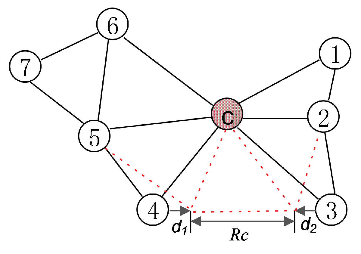
Figure 5 shows the 2-hop derived subgraph intention in k-hop local topology of a cut-point c. Arrows indicate the movement direction of UAV nodes based on predicted k-hop local topology and the red shadow node c is cut-point. The , . The distance of moving from node 4 to node 3 is and the distance from node 3 to node 4 is . Finally, the distance between node 3 and node 4 is , which forms a direct communication link. Changes of communication links after movement are shown as red dashed lines in Figure 6. If the link between node 3 and node 4 cannot be formed under the constraint of movement freedom degree, then node 4 and node 5 are regarded as a whole to recalculate the movement freedom degree in the direction and move again.
3.2.2. Only One Other Cut-Point in the 1-Hop Neighbor Nodes of Cut-Point c
Step 1: The cut-point c and its neighbor cut-point are regarded as a whole, and the remaining nodes in the topology are divided into several blocks where the nodes are connected.
Step 2: Under the constraint of movement freedom degree, according to the method in Case 1, the nodes except node c and are included into a connected set through the movement of nodes, and the two cut-points c and are “surrounded” to change two cut-points into non-cut points finally.
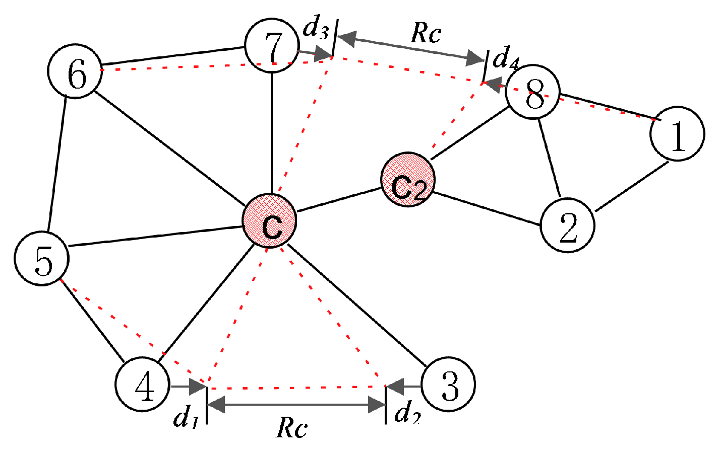
Figure 6 shows the 3-hop derived subgraph intention in k-hop local topology of a cut-point c. Arrows indicate the movement direction of UAV nodes based on predicted k-hop local topology, the red shadow node c and node are cut-points. The nodes outside the cut-points are divided into three sets , and . Under the constraint of the movement freedom degree of nodes, nodes 3 and 4 form direct communication link by moving in opposite directions. Similarly, direct communication link is formed between nodes 7 and 8. Changes of communication links after movement are shown as red dashed lines in Figure 6. The original links remain connected and the two cut-points of c and are changed into non-cut points.
3.2.3. Multiple Other Cut-Point in the 1-Hop Neighbor Nodes of Cut-Point c
Step 1: According to the method in Case 1, cut-point c and its neighbor cut-points are regarded as a whole. Change all cut-points into non-cut points. If fails, execute the following steps.
Step 2: Connecting the cut-points except the cut-point c, the rules of movement are the same as those of the previous two cases, following the constraint of movement freedom degree of nodes. If the communication link between the generalized leaf node and the cut-point is broken during the movement process, the generalized leaf nodes need to be moved to maintain the connection with the cut-point.
Step 3: Treat all cut-points as a whole and repeat the first step. Eventually “surround” all cut points and change all the cut-points into non-cut points.
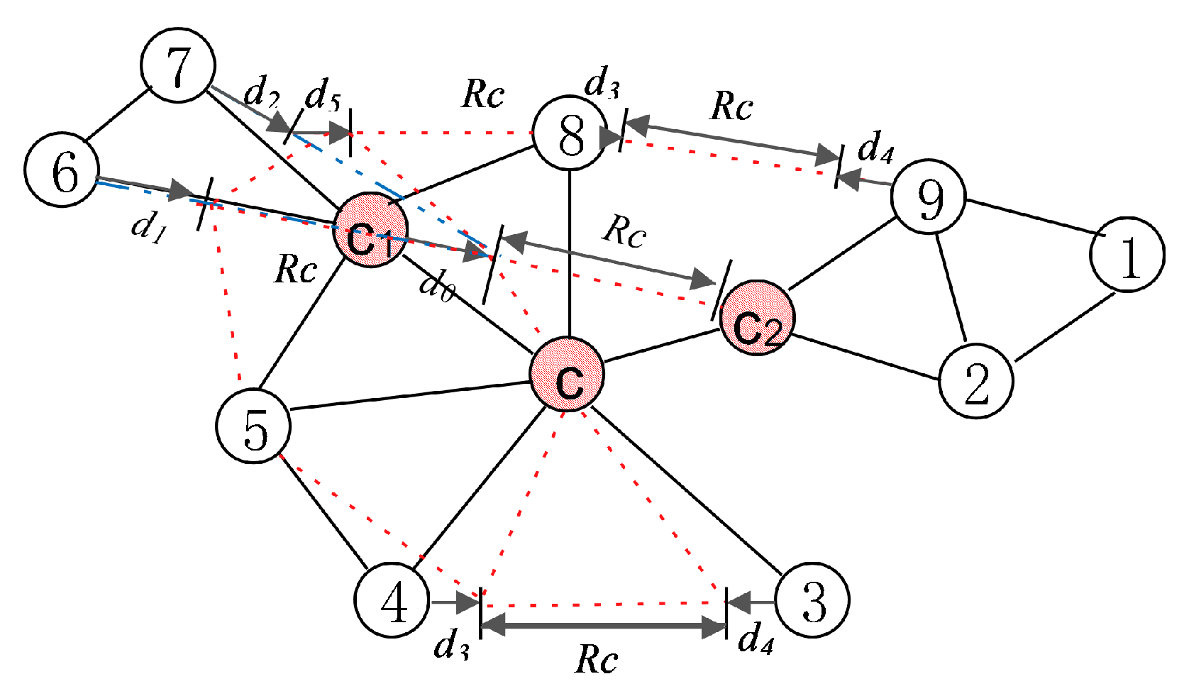
Figure 7 shows the 3-hop derived subgraph intention in k-hop local topology of a cut-point c and node 6 and node 7 are generalized leaf nodes. Arrows indicate the movement direction of UAV nodes based on predicted k-hop local topology and the red shadow node c, node and node are cut-points. If the first step fails, the cut-points and are moved to form a direct communication link, so that the other cut-points except cut point c are connected. However, the communication link between two generalized leaf nodes 6 and 7 and cut-point are disconnected. It is necessary to move node 6 and node 7 to maintain their link with the cut-point . Then, node 5 and node 6 can be connected exactly. Nodes except all the cut-points are divided into four sets , , , at this time. Under the constraint of movement freedom degree, node 3 and node 4 form direct communication link by moving in opposite directions. Similarly, direct communication link are formed between node 8 and node 9, and direct links are formed between node 7 and node 8. Changes of communication links after movement are shown as red dashed lines in Figure 7. The original links remain connected and the three cut-points c, and are changed into non-cut points.
3.3. Complexity Analysis
In k-hop topology of any node , the number of nodes is . The computation of constructing adjacency tables is . Assuming that the maximum connected block after removing node is and the number of nodes is . In the worst case, the cut-point detection algorithm needs to traverse the neighbors of all nodes in to get the DFS-tree set R. Therefore the computation of cut-point detection algorithm is shown in Equation (16).
where the network node density is constant.
In the process of establishing the model, it is necessary to calculate the movement freedom degree of all nodes in the -hop local topology of node and traverse all nodes and their neighbors. Therefore, the computation of establishing the movement freedom degree model is shown in Equation (17).
where is the number of nodes in -hop local topology of node .
When dividing the network into blocks, it is necessary to traverse all nodes and their neighbors excepting cut-points in . Therefore, the computation of partition is , where is the number of cut-points in . The computation of finding node pairs and that need moving is , where is the number of nodes in and is the number of nodes in during iteration. Therefore, the computation of updating the location of nodes in is shown in Equation (18).
In Cases 1 and 2, the computation of the LFTMF algorithm is shown in Equation (19).
In Case 3, in the worst case, the cut-points will also be involved in the deviation and the computation is shown in Equation (20).
In summary, . Therefore, the complexity of LFTMF algorithm is within .
4. Simulation Result
To verify the feasibility of the LFTMF algorithm and test its performance, we conducted simulation experiments to compare the performance of LFTMF algorithm, global block movement algorithm [17] and localized movement control algorithm [18]. The test simulated the application layer to transfer data and assumed an ideal MAC layer underneath, with no communication loss and instantaneous delivery of messages.
4.1. Simulation Environment and Parameter Setting
UAV carried out reconnaissance tasks in three-dimensional obstacle-free environment. UAV nodes were randomly distributed within a certain range, and the height distribution of the UAV cluster was kept within 100 m. UAV’s speed was 30 m/s, if it did not participate in the bi-connected fault-tolerant network adjustment. The UAV that participates in the adjustment can reach the destination on time during the adjustment period. The maximum communication range of UAV was m, and the duration of each topology update period was s. FANET was isomorphic and the initial network was single-connected.
4.2. Evaluating Indicator
Five hundred randomly single-connected network topologies were selected in the experiment and the number of maximum adjustment period was five equivalent to time t to time . The success rate of the achievement of fault-tolerant network, the average distance of deviation from original track, the ratio of nodes participating in cascade movement and the average adjustment period were taken as evaluation indexes. Definitions are as follows.
The consistency of k-hop cut-points and global cut-points is defined as the ratio of the number of global cut-points to the number of k-hop cut-points.
The success rate of achieving FANET fault-tolerant network () is defined as:
where is the total number of single-connected network topologies and B is the number of bi-connected fault-tolerant network topologies in five adjustment periods.
The average distance of deviation from original location () is also called average offset distance, which is the total distance that all UAV nodes deviate from their original track in the process of realizing a bi-connected fault-tolerant network in a single-connected network.
where is the location of every node in the adjusted UAV cluster, and is the original location of every node in the UAV cluster assuming no adjustment.
The ratio of UAV nodes participating in cascade movement () is defined as:
where is the number of nodes involved in cascade movement and is the total number of nodes in the network topology. reflects the degree of change in the original network topology, and has a great impact on computing and communication cost. The larger is the , the greater are the computing cost and communication cost.
The average adjustment period is the number of periods required for a single-connected network to become a bi-connected fault-tolerant network. The smaller is the , the smaller is the communication cost.
4.3. Discussion of Simulation Results
4.3.1. Experiment 1: Consistency of k-Hop Cut-Points and Global Cut-Points
The value of k was and the number of nodes . Simulated experiment of cut-points detection was carried in 500 random three-dimensional single-connected networks.
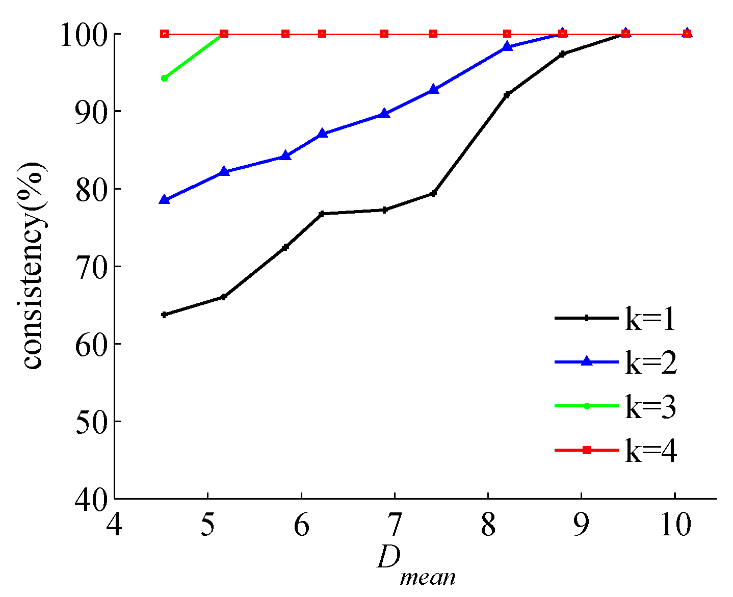
Figure 8 shows the relationship between the consistency of k-hop cut-points and global cut-points and network node density when k takes different values. With the increase of network node density, the consistency between k-hop cut-points and global cut-points increased. If the node degree were certain, the greater was the value of k, the greater was the consistency. The larger was the value of k, the higher was the communication cost. However, too small a value of k led to too many k-hop cut-points, which means non-global cut-points being recognized as global cut-points, resulting in unnecessary movement cost. Therefore, the value of k was 3 in subsequent experiments. It is worth noting that the global cut-points must be k-hop cut-points, so eliminating all k-hop cut-points means eliminating all global cut-points.
4.3.2. Experiment 2: With a Certain Number of UAV Nodes, Analyses of the Relationships among the Performances of LFTMF Algorithm, Global Block Movement Algorithm, Localized Movement Control Algorithm and the Network Node Density by Simulation
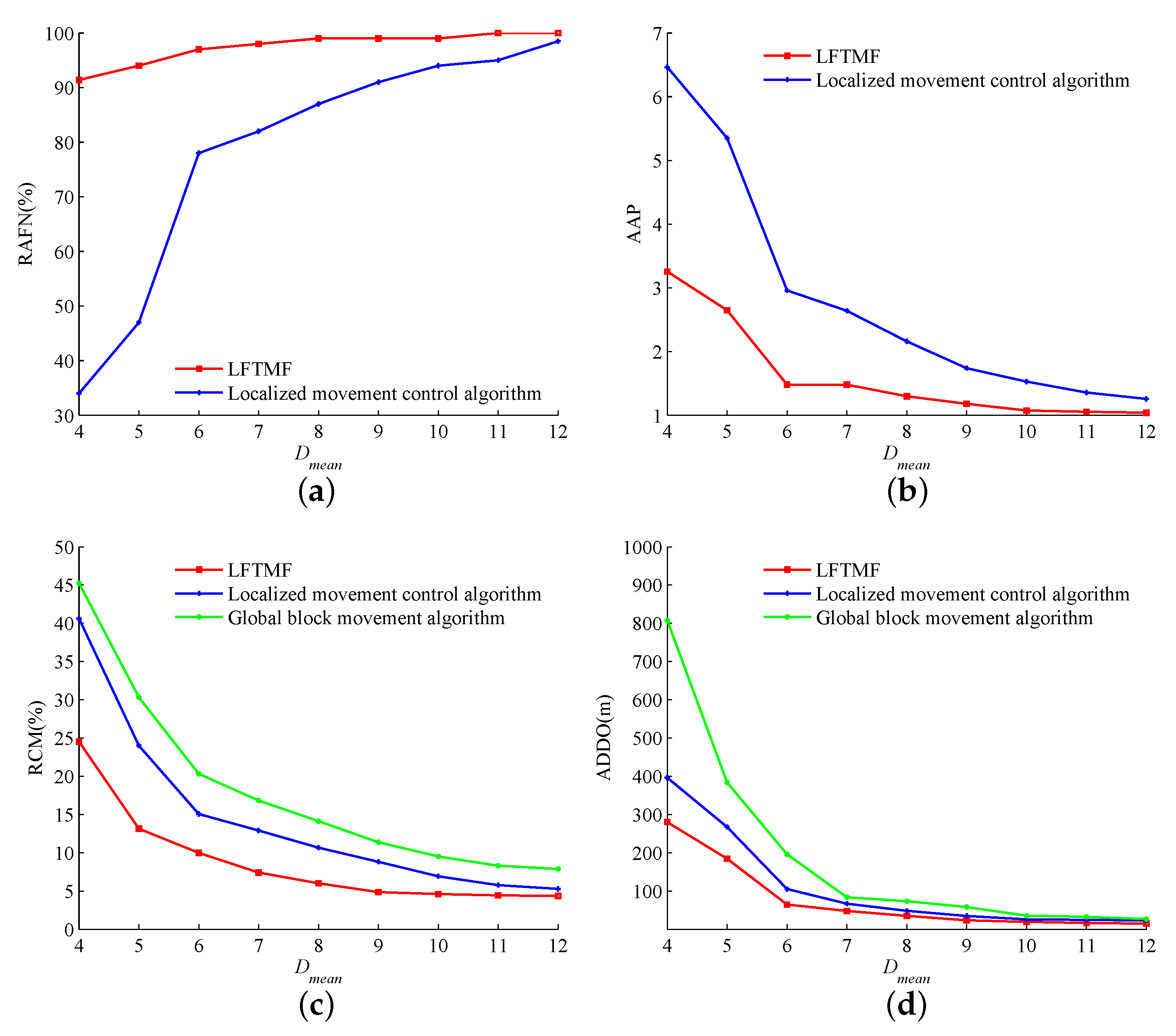
First, and the number of UAV nodes were set. Based on 500 random three-dimensional single-connected networks, the relationship between the performance of different algorithms and the network node density was tested, as shown in Figure 9.
A parse networks means . In Figure 9a, it can be seen that, when the network was sparse, the success rate of the achievement of bi-connected fault-tolerant network was more than 90%, while the success rate of the localized movement control algorithm was only 35–45%. When , the success rate of the localized movement control algorithm increased with the increase of , and finally reached more than 90%. in Figure 9b, it can be seen that, in sparse networks, the adjustment period of LFTMF algorithm was much shorter than that of localized movement control algorithm. With the increase of , the value of was close to 1, but the value of of LFTMF algorithm was always smaller than that of localized movement control algorithm.
The reasons for the above results are as follows. In sparse networks, there are many consecutive cut-points without the constraint of movement freedom degree in the localized movement control algorithm. The movement of some nodes leads to the disconnection of the original communication link and the generation of new cut-points. In LFTMF algorithm, the movement freedom degree of the third-hop node of cut-point is 0, and it does not participate in movement, forming a “barrier” to ensure the connectivity with the external topology. With the constraint of node freedom, no new cut-points will be generated. When the network node density is large, the number of cut-points is small, and both algorithms have higher success rate and smaller adjustment period.
In Figure 9c,d, it can be seen that the ratio of UAV nodes participating in cascade movement and average offset distance of the global block movement algorithm were larger than those of the two distributed algorithms. This is because the nodes move in blocks in block movement algorithm, resulting in more UAV nodes participating in the movement and a larger offset distance. Compared with LFTMF algorithm, localized movement control algorithm has a larger ratio of nodes participating in cascade movement and movement cost because it may lead to the generation of new cut-points, and the adjustment period is longer.
In summary, the performance of all the algorithms improved with the increase of network node density when the number of UAV nodes was certain. Compared with localized movement control algorithm, LFTMF algorithm has obvious advantages in sparse network.
4.3.3. Experiment 3: With a Certain Network Node Density, Analyses of the Relationships among the Performances of LFTMF Algorithm, Global Block Movement Algorithm, Localized Movement Control Algorithm and the Number of UAV Nodes by Simulation
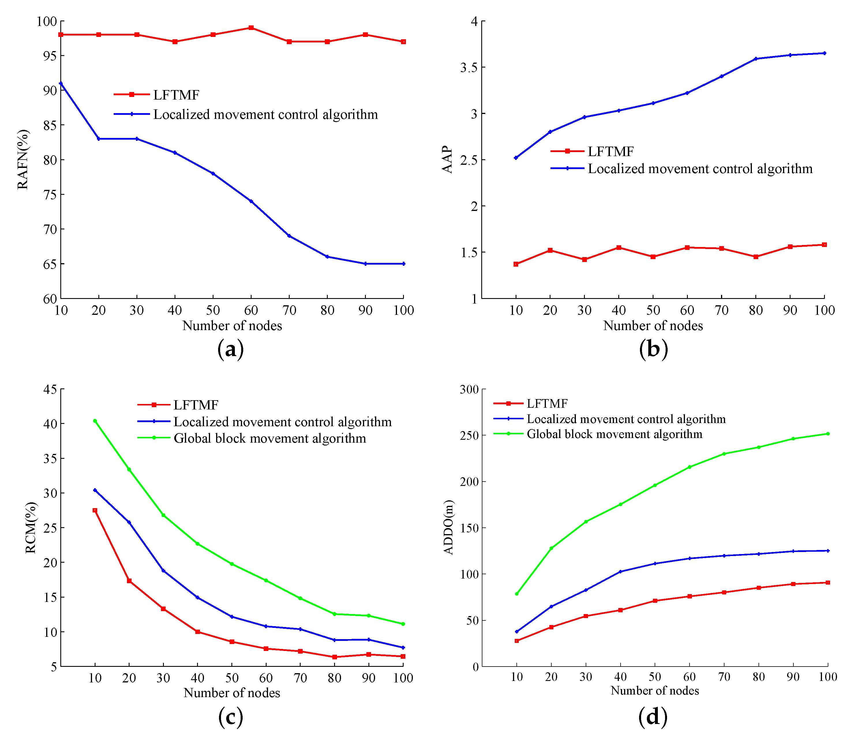
First, and the network node density were set. Based on 500 random three-dimensional single-connected networks, the relationship between the performance of different algorithms and the number of UAV nodes was tested, as shown in Figure 10.
It can be seen in Figure 10a,b that, with the increase of the number of nodes, the success rate of LFTMF algorithm remained above 95%, and the adjustment period was about 1.5, independent of the number of nodes. The success rate of the localized movement control algorithm decreased continuously, and finally stabilized at about 65%. The adjustment period increased continuously, and finally stabilized at about 3.5. The reasons is that, when the network scale increases, the 3-hop local topology cannot represent the global topology. Localized movement control algorithm will cause the disconnection between the local topology and the rest of the nodes in the global topology, resulting in new cut-points. When the number of nodes reached more than 80, the influence tended to be stable. In the LFTMF algorithm, the third-hop nodes of 3-hop local topology do not participate in the migration, and the movement freedom degree can effectively maintain the connectivity of the original link.
In Figure 10c,d, it can be seen that the performance of the local algorithm was better than that of the global block movement algorithm when the network scale was large, because the block movement algorithm participated in the movement as a block. The ratio of UAV nodes participating in cascade movement of the three algorithms decreased with the increase of network scale, and the average offset distance increased with the increase of network scale. The reason is that most of the nodes will participate in the movement when the network scale is small. Only the nodes around the cut-points participate in the movement when the network scale is large and at this point. The ratio of nodes participating in cascade movement is small, but the number of nodes involved in the movement increases leading to the increase of offset distance. Compared with localized movement control algorithm, the LFTMF algorithm had smaller ratio of participating in cascade movement and average offset distance.
In summary, when the network node density was certain, with the increase of network scale, the success rate of LFTMF algorithm in realizing bi-connected fault-tolerant network was always above 95%, and the overall performance was better than global block movement algorithm and localized movement control algorithm.
5. Conclusions
In this paper, we propose a localized fault-tolerant algorithm based on node movement freedom degree (LFTMF). The algorithm solves the problem that the single-connected FANET network is easily segmented due to the dynamic characteristics of the UAVs. In three-dimensional FANET, we establish the movement freedom degree model, and propose three movement strategies according to the distribution of cut-points in the k-hop local topology of cut-points. The performance of LFTMF algorithm in three-dimensional FANET network was studied by numerical simulation. The simulation results show that, compared with localized movement control algorithm and global block movement algorithm, the proposed algorithm improves the success rate of the achievement of bi-connected fault-tolerant network under the constraint of movement freedom degree, and has smaller adjustment period, offset distance and the ratio of nodes of participating in cascade movement, maintaining the connectivity of the original link at the same time. The performance advantage of this algorithm is particularly prominent when the network is sparse or the network scale is large. This topology control algorithm has potential application prospects in network fault-tolerant control.
Author Contributions
Conceptualization, Q.G. and J.Y.; Methodology, Q.G. and J.Y.; Software, J.Y.; Validation, Q.G. and J.Y.; Supervision W.X., Writing—original draft, J.Y.; and Writing—review and editing, J.Y. and W.X.
Funding
This research was funded by the Central University Basic Research Business Expenses Special Fund Project (No.HEUCFG201832), the National Key Research and Development Program of China (No.2016YFC0101700), the Heilongjiang Province Applied Technology Research and Development Program National Project Provincial Fund (No.GX16A007), State Key Laboratory Open Fund (No.702SKL201720), and the International S&T Cooperation Program of China (ISTCP) (No. 2015DFR10220).
Acknowledgments
The authors would like to thank the editors and the reviewers for their comments on a draft of this article.
Conflicts of Interest
The authors declare no conflict of interest.
References
- Gupta, L.; Jain, R.; Vaszkun, G. Survey of Important Issues in UAV Communication Networks. IEEE Commun. Surv. Tutor. 2015, 18, 1123–1152. [Google Scholar] [CrossRef]
- İlker, B.; Sahingoz, O.K.; Şamil, T. Flying Ad-Hoc Networks (FANETs): A survey. Ad Hoc Netw. 2015, 11, 1254–1270. [Google Scholar]
- Peng, W.; Dong, G.; Yang, K.; Su, J. A Random Road Network Model and Its Effects on Topological Characteristics of Mobile Delay-Tolerant Networks. IEEE Trans. Mob. Comput. 2014, 13, 2706–2718. [Google Scholar] [CrossRef]
- Liu, X. Survivability-aware connectivity restoration for partitioned wireless sensor networks. IEEE Commun. Lett. 2017, 33, 2444–2447. [Google Scholar] [CrossRef]
- Liu, H.; Yoo, S.-J.; Kwak, K.S. Opportunistic relaying for low-altitude UAV swarm secure communications with multiple eavesdroppers. IEEE Commun. Surv. Tutor. 2018, 20, 496–508. [Google Scholar] [CrossRef]
- Ling, C.; Jiahong, L.; Zhiwei, H.; Wu, B. Movement control algorithm of fault-tolerant UAVs Ad Hoc networks. J. Natl. Univ. Def. Technol. 2012, 33, 58–62. [Google Scholar]
- Shi, Y.; Sun, H.; Sheng, M.; Li, J.; Li, X. Constructing a Robust Topology for Reliable Communications in Multi-Channel Cognitive Radio Ad Hoc Networks. IEEE Commun. Mag. 2018, 56, 172–179. [Google Scholar] [CrossRef]
- Chang, Y.; Yuan, X.; Al-Dhahir, N. A Joint Unsupervised Learning and Genetic Algorithm Approach for Topology Control in Energy-Efficient Ultra-Dense Wireless Sensor Networks. IEEE Commun. Lett. 2018, 22, 2370–2373. [Google Scholar] [CrossRef]
- Koti, R.B.; Kakkasageri, M.S. Dynamic topology control in multiple clustered vehicular ad hoc networks. In Proceedings of the 2016 International Conference on Signal Processing, Communication, Power and Embedded System (SCOPES), Paralakhemundi, India, 3–5 October 2016; pp. 1371–1375. [Google Scholar]
- Aznar, F.; Pujol, M.; Aldeguer, R.R.; Pujol, F.A. Energy-Efficient Swarm Behavior for Indoor UAV Ad-Hoc Network Deployment. Symmetry 2018, 10, 632. [Google Scholar] [CrossRef]
- Ramanathan, R.; Rosales-Hain, R. Topology control of multihop wireless networks using transmit power adjustment. IEEE Comput. Commun. Soc. 2000, 33, 404–413. [Google Scholar]
- Ahmed, S.; Rahman, K.A.; Rubeaai, S.A. A delay-tolerant network architecture for challenged internets. In Proceedings of the 2003 Conference on Applications, Technologies, Architectures, and Protocols for Computer Communications, Karlsruhe, Germany, 25–29 August 2003; pp. 129–133. [Google Scholar]
- Mozaffari, M.; Saad, W.; Bennis, M.; Debbah, M. Unmanned Aerial Vehicle with Underlaid Device-to-Device Communications: Performance and Tradeoffs. IEEE Trans. Wirel. Commun. 2016, 15, 3949–3963. [Google Scholar] [CrossRef]
- Lagum, F.; Bor-Yaliniz, I.; Yanikomeroglu, H. Strategic densification with UAV-BSs in cellular networks. IEEE Wirel. Commun. Lett. 2018, 7, 384–387. [Google Scholar] [CrossRef]
- Zhang, Z.; Zhao, J. Relay route planning based on connectivity in airborne ad hoc networks. In Proceedings of the 2017 29th Chinese Control And Decision Conference (CCDC), Chongqing, China, 28–30 May 2017; pp. 1948–9447. [Google Scholar]
- Ling, C.; Jiahong, L.; Zhiwei, H. Fault tolerant relay node placement in UAVs Ad hoc networks. Syst. Eng. Electron. 2012, 34, 179–184. [Google Scholar]
- Kashyap, A.; Khuller, S.; Shayman, M. Relay placement for fault tolerance in wireless networks in higher dimensions. Comput. Geom. 2011, 44, 206–215. [Google Scholar] [CrossRef] [Green Version]
- Jie, L.I.; Gong, E.; Sun, Z. Relay speed control for realization of fault-tolerant aeronautical ad hoc networks. J. Natl. Univ. Def. Technol. 2015, 37, 158–164. [Google Scholar]
- Song, X.; Zhou, L.; Zhao, H. Localized Fault Tolerant and Connectivity Restoration Algorithms in Mobile Wireless Ad Hoc Network. IEEE Access 2018, 6, 36469–36478. [Google Scholar] [CrossRef]
- Prithwish, B.; Jason, R. Movement control algorithms for realization of fault tolerant Ad Hoc networks. IEEE Netw. 2004, 18, 36–44. [Google Scholar]
- Shantanu, D.; Hai, L.; Amiya, N.; Stojmenović, I. A Localized algorithm for bi-connectivity of connected mobile robots. Telecommun. Syst. 2009, 40, 129–140. [Google Scholar]
- Liu, H.; Chu, X.; Leung, Y.W. Simple movement control algorithm for bi-connectivity in robotic sensor networks. IEEE J. Sel. Areas Commun. 2010, 28, 994–1005. [Google Scholar] [CrossRef] [Green Version]
Figure 1.
FANET Network topology diagram.

Figure 2.
Fault-tolerant network topology control flow chart.

Figure 3.
Flow chart of cut point detection algorithm based on k-hop local topology.

Figure 4.
Realization of bi-connected fault-tolerant networks by adjusting the movement directions of some nodes.
Figure 4.
Realization of bi-connected fault-tolerant networks by adjusting the movement directions of some nodes.

Figure 5.
Local topology sketch of single cut-point.

Figure 6.
Local topology sketch of cut-point c with only one neighbor as cut-point.

Figure 7.
Local topology sketch of cut-point c with multiple neighbors as cut-points.

Figure 8.
The relationship between the consistency of k-hop cut-points and global cut-points and network node density with different values of k.
Figure 8.
The relationship between the consistency of k-hop cut-points and global cut-points and network node density with different values of k.

Figure 9.
This figure shows the the relationship between the performance of different algorithms and the network node density when the number of UAV nodes is certain: (a) the success rate of the achievement of bi-connected fault-tolerant network, RAFN; (b) the adjustment period, AAP; (c) the ratio of UAV nodes participating in cascade movement, RCM; and (d) average offset distance, ADDO.

Figure 10.
This figure shows the the relationship between the performance of different algorithms and the number of UAV nodes when the the network node density is certain: (a) The success rate of the achievement of bi-connected fault-tolerant network, RAFN; (b) the adjustment period, AAP; (c) the ratio of UAV nodes participating in cascade movement, RCM; and (d) average offset distance, ADDO.


Table 1.
Partial symbols and their definitions.
| Symbols | Definitions |
|---|---|
| The time for each adjustment period. | |
| Location of UAV Node at time t. | |
| Predictive Location of UAV at time in k-hop local topology. | |
| The calculated Location of UAV in k-hop local topology at time . | |
| Distance between UAV Nodes and . | |
| The set of neighbor nodes of UAV . | |
| Set of k-hop neighbor nodes of UAV . | |
| Closed set of neighbors of UAV , . | |
| Network node density. |
© 2019 by the authors. Licensee MDPI, Basel, Switzerland. This article is an open access article distributed under the terms and conditions of the Creative Commons Attribution (CC BY) license (http://creativecommons.org/licenses/by/4.0/).
Share and Cite
MDPI and ACS Style
Guo, Q.; Yan, J.; Xu, W. Localized Fault Tolerant Algorithm Based on Node Movement Freedom Degree in Flying Ad Hoc Networks. Symmetry 2019, 11, 106. https://0-doi-org.brum.beds.ac.uk/10.3390/sym11010106
AMA Style
Guo Q, Yan J, Xu W. Localized Fault Tolerant Algorithm Based on Node Movement Freedom Degree in Flying Ad Hoc Networks. Symmetry. 2019; 11(1):106. https://0-doi-org.brum.beds.ac.uk/10.3390/sym11010106
Chicago/Turabian StyleGuo, Qiang, Jichen Yan, and Wei Xu. 2019. "Localized Fault Tolerant Algorithm Based on Node Movement Freedom Degree in Flying Ad Hoc Networks" Symmetry 11, no. 1: 106. https://0-doi-org.brum.beds.ac.uk/10.3390/sym11010106
Note that from the first issue of 2016, this journal uses article numbers instead of page numbers. See further details here.