Using Stochastic Decision Networks to Assess Costs and Completion Times of Refurbishment Work in Construction


Abstract
:1. Introduction
- The complicated course of design work and the unpredictable process of obtaining legal opinions and approvals of proposed refurbishment solutions, the lack of approval of design solutions by architectural conservation authorities.
- Difficulty in determining the scope of work (a high probability of additional or replacement types of work) due to the limited identification of the structure of an existing building, e.g., the technical condition of foundations uncovered while performing construction work can require different forms of reinforcing them.
- In the case of historical buildings, it is possible that discoveries will be made during construction work, resulting in additional archaeological digs, as well as more construction and conservation work [4], e.g., the replacement of existing plasters on a historical structure can result in the discovery of polychromes underneath.
1.1. Stochastic Networks—Literature Review
1.2. Decision Networks—Literature Review
1.3. Research Aims
- An innovative approach to planning the restoration of buildings, allowing for the consideration of various completion scenarios, the occurrence of which can be both random and decision-based. The following will be required for this goal to be achieved:
- Defining the stochastic-decision structure of the network model containing an appropriate topology of vertices with deterministic, stochastic and decision emitters (as a directed, non-cyclical graph, with one initial vertex and numerous final end vertices).
- Developing a nonlinear one-and multi-criteria binary programming model for the purpose of optimising (in the time-cost aspect) various scenarios of the carrying out of the project that is being modelled by the network.
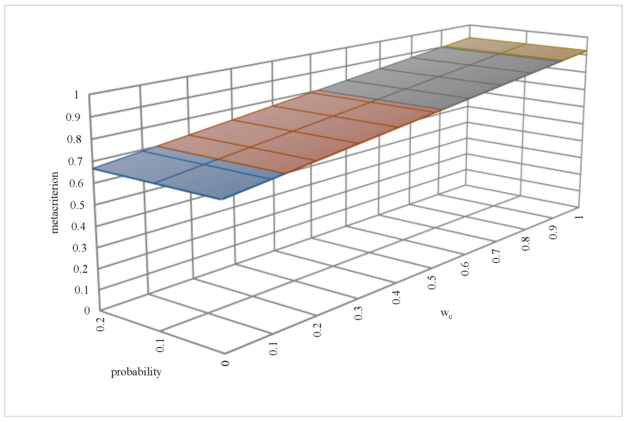
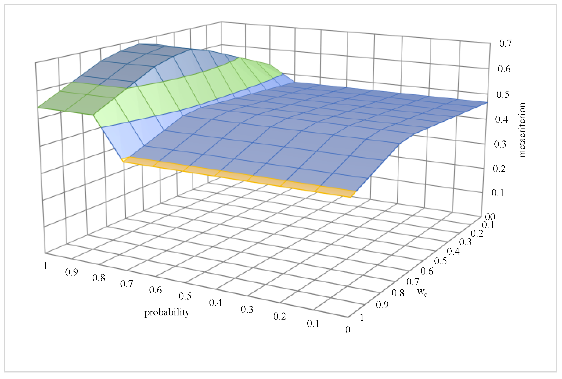
- As a result, the decision-maker, by specifying their preferences as to the planned result of a project and their risk aversion, will receive an optimal (in terms of expected time and costs) scenario of carrying out their project. In the case of a multi-criteria analysis (time and cost), the decision-maker will also be able to specify different values of weights for the expected time and cost of the planned project in the goal function. As a part of the results, the decision-maker will also obtain information on the type of technical solutions or the manner of carrying out the work that should be included in the plan of the optimal scenario of carrying out the project.
- Developing a digital application of the approach and performing a calculation experiment within which the effectiveness of the stochastic decision network will be demonstrated in relation to the traditional approach.
2. Method
2.1. Definition of the Structure of a Stochastic Decision Network
- Receivers, defining the conditions for achieving a given state (receiver activation);
- Emitters, specifying the conditions for the carrying out of specific arcs that originate from it (Table 1).
2.2. Optimisation Model
- The shortest expected completion time of the scenario of the planned project;
- The lowest expected cost of the carrying out of the scenario of the planned project;
- The shortest completion time and lowest cost of the carrying out of the scenario of the planned project.
- —starting vertex,
- —end vertex,
- —any other vertex,
- —set of permissible solutions
- —set of direct successors
- —collection of direct predecessors of r
- —out-degree (number of actions (arcs) exiting a vertex r)
- —in-degree (number of actions (arcs) entering a vertex )
- —binary decision variable determining the existence of the i-j action
- —probability of i-j action
- —accumulated probability of the occurrence of i-j action (taking into account the probability of the occurrence of preceding tasks)
- —probability of the occurrence of vertex
- —the cost of action i-j
- —duration of action i-j—weights for the criteria of time and cost, respectively
- —required probability of occurrence of the final node
- —expected completion time of vertex
- —expected cost of completing vertex r
3. Calculation Experiment
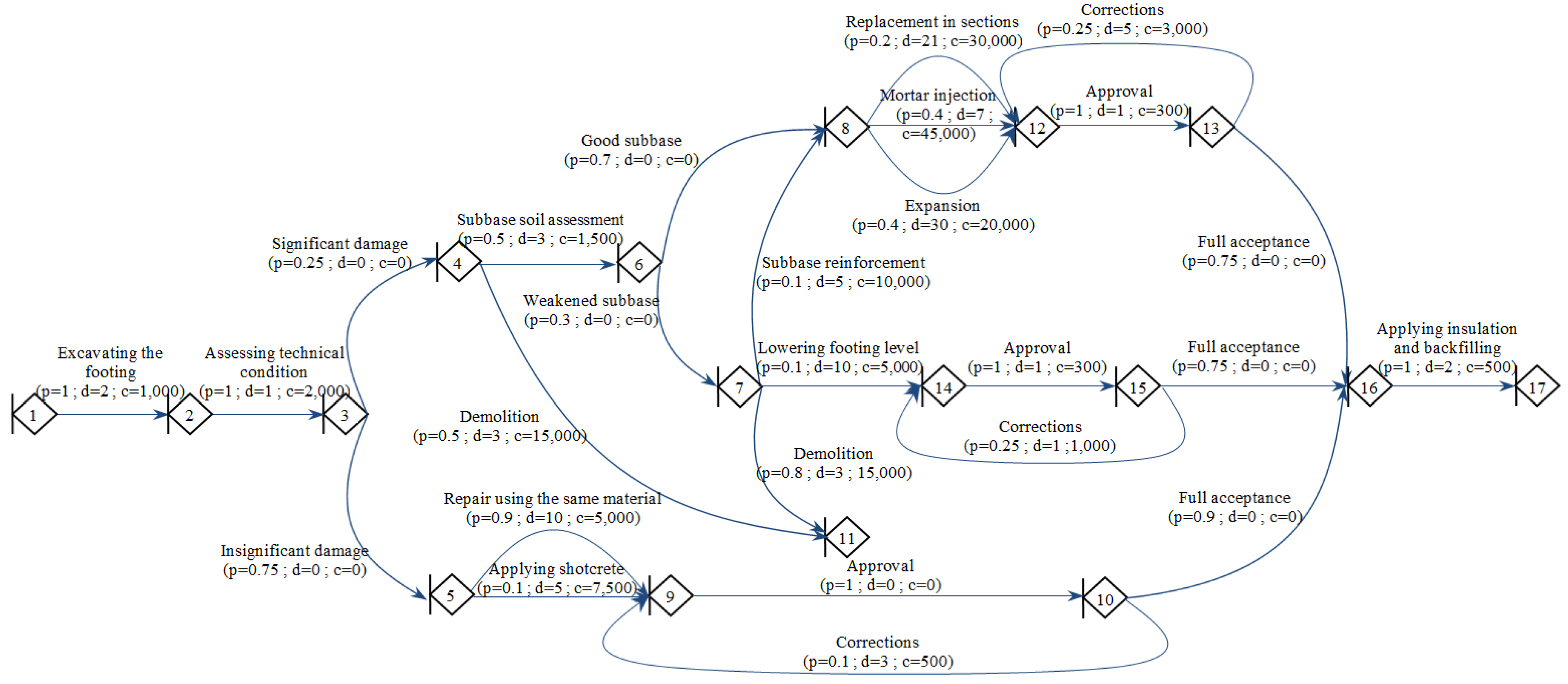
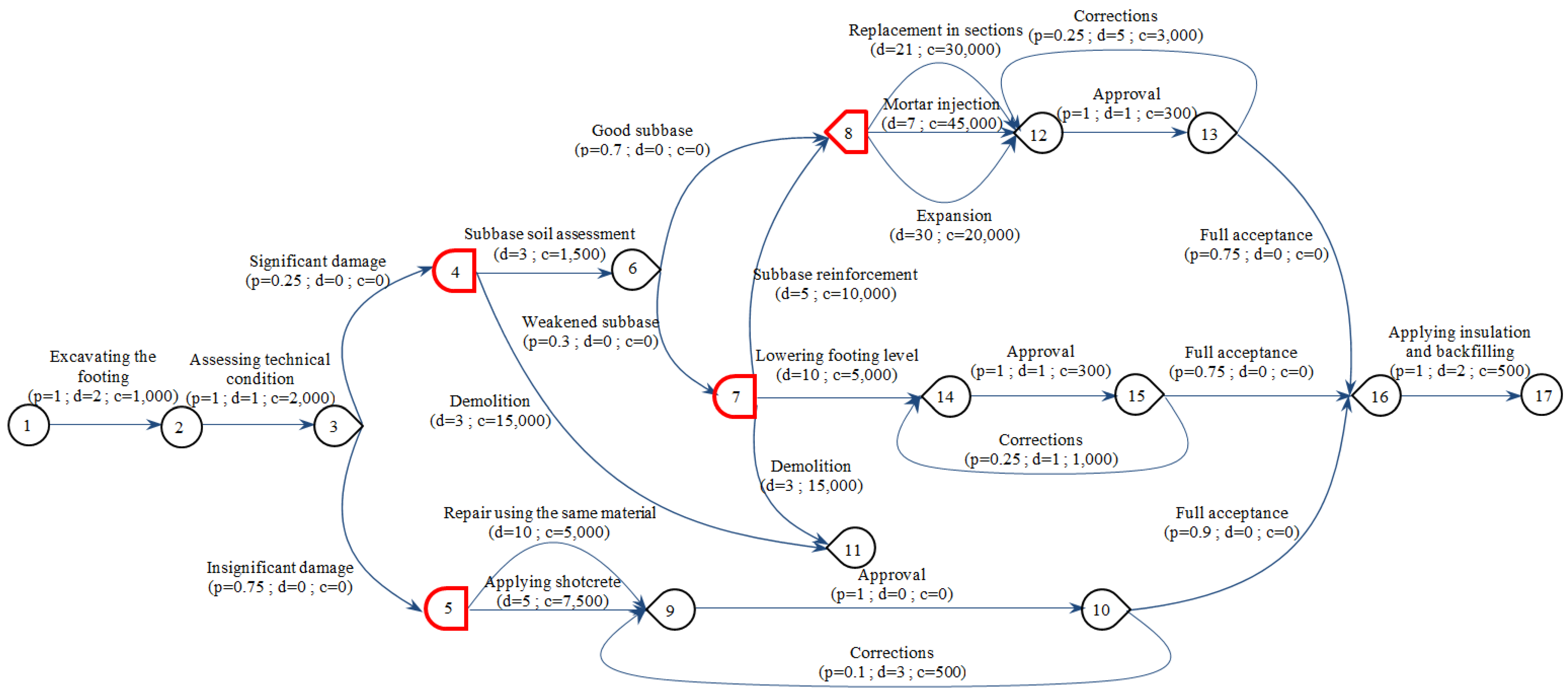
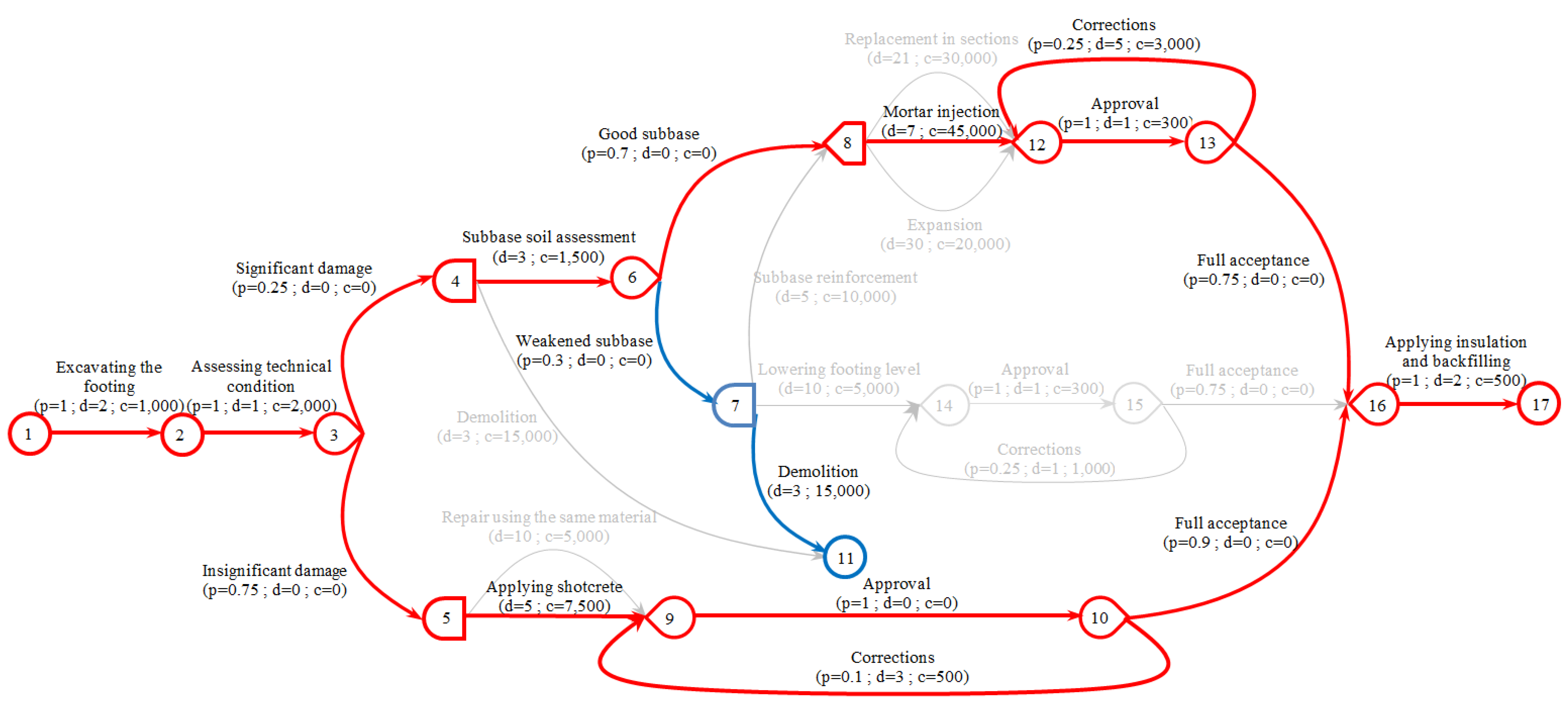
3.1. Construction of a Stochastic Decision Network Model
3.2. Analysis of the Network Model
- Brute force;
- APOPT solver (for Advanced Process OPTIMIZER) is a software package for solving large-scale optimisation problems (http://apopt.com/). The program is used to solve linear problems (LP), square (QP), non-linear (NLP) and mixed problems (MIP, MILP, MINLP). The APOPT solver was used with the APMonitor service [37].
4. Analysis of Results
5. Conclusions and Discussion
Author Contributions
Funding
Conflicts of Interest
References
- Zavadskas, E.K.; Antucheviciene, J. Development of an indicator model and ranking of sustainable revitalization alternatives of derelict property: A Lithuanian case study. Sustain. Dev. 2006, 14, 287–299. [Google Scholar] [CrossRef]
- Zavadskas, E.K.; Antucheviciene, J. Multiple criteria evaluation of rural building’s regeneration alternatives. Build. Environ. 2007, 42, 436–451. [Google Scholar] [CrossRef]
- European Union Treaty of Lisbon Amending the Treaty on European Union and the Treaty establishing the European Community. 2007. Available online: http://data.europa.eu/eli/treaty/lis/sign (accessed on 28 January 2019).
- Śladowski, G.; Radziszewska-Zielina, E. Description of technological and organisational problems in construction works using the example of restoration of the outer courtyard on Wawel Hill. Tech. Trans. 2015, 2, 117–125. [Google Scholar]
- Radziszewska-Zielina, E.; Kutut, V.; Mesároš, P.; Sroka, B.; Szewczyk, B.; Śladowski, G. Problems of assessing the duration and cost of restoration projects on the example of Poland, Slovakia and Lithuania. Sci. Rev. Eng. Environ. Sci. 2018, 27, 3–8. [Google Scholar] [CrossRef] [Green Version]
- Lootsma, F.A. Theory and Methodology stochastic and fuzzy PERT. Eur. J. Oper. Res. 1989, 143, 174–183. [Google Scholar] [CrossRef]
- Chanas, S.; Zieliński, P. Critical path analysis in the network with fuzzy activity times. Fuzzy Sets Syst. 2001, 122, 195–204. [Google Scholar] [CrossRef]
- Lin, F.T.; Yao, J.S. Fuzzy critical path method based on signed-distance ranking and statistical confidence-interval estimates. J. Supercomput. 2003, 24, 305–325. [Google Scholar] [CrossRef]
- Chen, C.-T.; Huang, S.-F. Applying fuzzy method for measuring criticality in project network. Inf. Sci. 2007, 177, 2448–2458. [Google Scholar] [CrossRef]
- Hajdu, M. Effects of the application of activity calendars on the distribution of project duration in PERT networks. Autom. Constr. 2013, 35, 397–404. [Google Scholar] [CrossRef]
- Radziszewska-Zielina, E.; Śladowski, G.; Sibielak, M. Planning the reconstruction of a historical building by using a fuzzy stochastic network. Autom. Constr. 2017, 84, 242–257. [Google Scholar] [CrossRef]
- Eisner, H. A Generalized Network Approach to the Planning and Scheduling of a Research Project. Oper. Res. 1962, 10, 115–125. [Google Scholar] [CrossRef]
- Pritsker, A.A.B. GERT: Graphical Evaluation and Review Technique; Rand Corporation: Santa Monica, CA, USA, 1966. [Google Scholar]
- Whitehouse, G.E. Systems Analysis and Design Using Network Techniques; Prentice-Hall: Englewood Cliffs, NJ, USA, 1973. [Google Scholar]
- Cheng, C.-H. Fuzzy consecutive-k-out-of-n:F system reliability. Microelectron. Reliab. 1994, 34, 1909–1922. [Google Scholar] [CrossRef]
- Cheng, C.-H. Fuzzy repairable reliability based on fuzzy gert. Microelectron. Reliab. 1996, 36, 1557–1563. [Google Scholar] [CrossRef]
- Gavareshki, M.K. New fuzzy GERT method for research projects scheduling. In Proceedings of the 2004 IEEE International Engineering Management Conference, Singapore, 18–21 October 2004; Volume 2, pp. 820–824. [Google Scholar]
- Hashemin, S.S. Fuzzy completion time for alternative stochastic networks. J. Ind. Eng. Int. 2010, 6, 17–22. [Google Scholar]
- Norouzi, G.; Heydari, M.; Noori, S.; Bagherpour, M. Developing a mathematical model for scheduling and determining success probability of research projects considering complex-fuzzy networks. J. Appl. Math. 2015. [Google Scholar] [CrossRef]
- Zadeh, L.A. Fuzzy sets. Inf. Control 1965, 8, 338–354. [Google Scholar] [CrossRef]
- Zanddizari, M. Set confidence interval for customer order cycle time in supply chain using GERT method. In Proceedings of the 17th IASTED international Conference on Modelling and Simulation, Montreal, QC, Canada, 24–26 May 2006; pp. 213–218. [Google Scholar]
- Aytulun, S.K.; Guneri, A.F. Business process modelling with stochastic networks. Int. J. Prod. Res. 2008, 46, 2743–2764. [Google Scholar] [CrossRef]
- Zhang, Z.; Ye, W.; Xia, Z. Research on A GERT Based Risk Transfer Model in Complex Product Development Process. J. Grey Syst. 2015, 27, 99–111. [Google Scholar]
- Nelson, R.G.; Azaron, A.; Aref, S. The use of a GERT based method to model concurrent product development processes. Eur. J. Oper. Res. 2016, 250, 566–578. [Google Scholar] [CrossRef]
- Kosecki, A. Use of stochastic network models in managing the renovation and rehabilitation projects. In Integrated Approaches to the Design and Management of Buildings Reconstruction: International University Textbook; EuroScientia: Wambeek, Belgium, 2014; pp. 52–60. [Google Scholar]
- Hougui, Z. Study on stochastic model for the construction of concrete longitudinal cofferdam in the Three Gorges Project. J. Hydraul. Eng. 1997, 8, 57–60. [Google Scholar]
- Pena-Mora, F.; Li, M. Dynamic planning and control methodology for design/build fast-track construction projects. J. Constr. Eng. Manag. 2001, 127, 1–17. [Google Scholar] [CrossRef]
- Gao, X.; Shen, Y.; Lin, J. Schedule risk management at early stages of large construction projects based on the GERT model. In Proceedings of the IEEE Conference Anthology, Shenyang, China, 7–9 November 2014; pp. 1–4. [Google Scholar]
- Wang, B.; Li, Z.; Gao, J.; Vaso, H. Critical Quality Source Diagnosis for Dam Concrete Construction Based on Quality Gain-loss Function. J. Eng. Sci. Technol. Rev. 2014, 7, 137–151. [Google Scholar] [CrossRef]
- Ignasiak, E. Optymalne struktury projektów w sieciach alternatywno-decyzyjnych (Optimal project structures in alternative-decision networks). Prz. Stat. (Stat. Rev.) 1975, 22, 323–333. [Google Scholar]
- Śladowski, G. Modeling technological and organizational variants of building projects. Tech. Trans. 2014, 5, 261–269. [Google Scholar]
- Zhang, L.H.; Liu, X.; Zhong, G. Bound Duration Theorem and DCPM Network Reduction. In Proceedings of the 2009 International Conference on Electronic Commerce and Business Intelligence, Beijing, China, 6–7 June 2009; pp. 230–233. [Google Scholar]
- Zhang, L.; Meng, X.; Cui, L. New Method for DCPM by Substituting Critical Path. In Proceedings of the 2011 International Conference on Management and Service Science, Wuhan, China, 12–14 August 2011; pp. 1–4. [Google Scholar]
- Ibadov, N. The Alternative Net Model with the Fuzzy Decision Node for the Construction Projects Planning. Arch. Civ. Eng. 2018, 64, 3–20. [Google Scholar] [CrossRef]
- Ibadov, N.; Kulejewski, J. Construction projects planning using network model with the fuzzy decision node. Int. J. Environ. Sci. Technol. 2019, 1–8. [Google Scholar] [CrossRef]
- Więckowski, A. Principles of the NNM method applied in the analysis of process realisation. Autom. Constr. 2002, 11, 409–420. [Google Scholar] [CrossRef]
- Hedengren, J.D.; Shishavan, R.A.; Powell, K.M.; Edgar, T.F. Nonlinear modeling, estimation and predictive control in APMonitor. Comput. Chem. Eng. 2014, 70, 133–148. [Google Scholar] [CrossRef]
- Shang, Y. Subgraph Robustness of Complex Networks Under Attacks. IEEE Trans. Syst. Man Cybern. Syst. 2017, 99, 1–12. [Google Scholar] [CrossRef]
- Rizzo, F.; Caracoglia, L.; Montelpare, S. Predicting the flutter speed of a pedestrian suspension bridge through examination of laboratory experimental errors. Eng. Struct. 2018, 172, 589–613. [Google Scholar] [CrossRef]
- Shang, Y. Distinct Clusterings and Characteristic Path Lengths in Dynamic Small-World Networks with Identical Limit Degree Distribution. J. Stat. Phys. 2012, 149, 505–518. [Google Scholar] [CrossRef]
- Shang, Y. Geometric Assortative Growth Model for Small-World Networks. Sci. World J. 2014, 2014, 1–8. [Google Scholar] [CrossRef] [PubMed]
- Shang, Y. On the likelihood of forests. Phys. A Stat. Mech. Its Appl. 2016, 456, 157–166. [Google Scholar] [CrossRef]


| The Name of the Receiver/Emitter | Graphical Representation of the Form of Logical Reception and Emission of Activities (Arches) | Conditions for the Reception and Emission of Activities (arcs) within the Structure of the Network |
|---|---|---|
| Receiver “AND” |  | The “AND” receiver of vertex y will be activated if and only if all the actions of entering it will be completed. |
| Receiver “inclusive-or IOR” |  | The receiver “or” of vertex y will be activated if and only if at least one of the actions entering it will be completed. |
| Emitter “deterministic” |  | The deterministic emitter of vertex y enables the carrying out of all actions from it, provided that the vertex has been activated. |
| Emitter “stochastic” |  | The stochastic emitter of vertex y allows the performance of only one of the actions from it with a certain probability, provided that the node has been activated. At the same time, the condition must be met where: is a set of direct successors. |
| Emitter “decision” |  | The y-vertex decision emitter only allows one of the actions that are outbound from it, provided that the vertex has been activated. The decision maker determines which task/action will be carried out. |
| Receiver | AND | Inclusive-Or IOR | |
|---|---|---|---|
| Emitter | |||
| deterministic |  |  | |
| stochastic |  |  | |
| decision |  |  | |
| 1 | 2 | 3 | 4 | 5 | 6 | 7 | 8 | 9 | 10 | 11 | 12 | 13 | 14 | 15 | 16 | 17 | 18 | 19 | 20 | ||
|---|---|---|---|---|---|---|---|---|---|---|---|---|---|---|---|---|---|---|---|---|---|
| i-j | |||||||||||||||||||||
| 1–2 | 1 | 1 | 1 | 1 | 1 | 1 | 1 | 1 | 1 | 1 | 1 | 1 | 1 | 1 | 1 | 1 | 1 | 1 | 1 | 1 | |
| 2–3 | 1 | 1 | 1 | 1 | 1 | 1 | 1 | 1 | 1 | 1 | 1 | 1 | 1 | 1 | 1 | 1 | 1 | 1 | 1 | 1 | |
| 3–4 | 1 | 1 | 1 | 1 | 1 | 1 | 1 | 1 | 1 | 1 | 1 | 1 | 1 | 1 | 1 | 1 | 1 | 1 | 1 | 1 | |
| 3–5 | 1 | 1 | 1 | 1 | 1 | 1 | 1 | 1 | 1 | 1 | 1 | 1 | 1 | 1 | 1 | 1 | 1 | 1 | 1 | 1 | |
| 4–6 | 0 | 0 | 1 | 1 | 1 | 1 | 1 | 1 | 1 | 1 | 1 | 1 | 1 | 1 | 1 | 1 | 1 | 1 | 1 | 1 | |
| 4–11 | 1 | 1 | 0 | 0 | 0 | 0 | 0 | 0 | 0 | 0 | 0 | 0 | 0 | 0 | 0 | 0 | 0 | 0 | 0 | 0 | |
| 5–9 | 1 | 0 | 1 | 1 | 1 | 1 | 1 | 1 | 1 | 1 | 1 | 0 | 0 | 0 | 0 | 0 | 0 | 0 | 0 | 0 | |
| 5–9 | 0 | 1 | 0 | 0 | 0 | 0 | 0 | 0 | 0 | 0 | 0 | 1 | 1 | 1 | 1 | 1 | 1 | 1 | 1 | 1 | |
| 6–7 | 0 | 0 | 1 | 1 | 1 | 1 | 1 | 1 | 1 | 1 | 1 | 1 | 1 | 1 | 1 | 1 | 1 | 1 | 1 | 1 | |
| 6–8 | 0 | 0 | 1 | 1 | 1 | 1 | 1 | 1 | 1 | 1 | 1 | 1 | 1 | 1 | 1 | 1 | 1 | 1 | 1 | 1 | |
| 7–8 | 0 | 0 | 1 | 1 | 1 | 0 | 0 | 0 | 0 | 0 | 0 | 1 | 1 | 1 | 0 | 0 | 0 | 0 | 0 | 0 | |
| 7–11 | 0 | 0 | 0 | 0 | 0 | 1 | 1 | 1 | 0 | 0 | 0 | 0 | 0 | 0 | 1 | 1 | 1 | 0 | 0 | 0 | |
| 7–14 | 0 | 0 | 0 | 0 | 0 | 0 | 0 | 0 | 1 | 1 | 1 | 0 | 0 | 0 | 0 | 0 | 0 | 1 | 1 | 1 | |
| 8–12 | 0 | 0 | 1 | 0 | 0 | 1 | 0 | 0 | 1 | 0 | 0 | 1 | 0 | 0 | 1 | 0 | 0 | 1 | 0 | 0 | |
| 8–12 | 0 | 0 | 0 | 1 | 0 | 0 | 1 | 0 | 0 | 1 | 0 | 0 | 1 | 0 | 0 | 1 | 0 | 0 | 1 | 0 | |
| 8–12 | 0 | 0 | 0 | 0 | 1 | 0 | 0 | 1 | 0 | 0 | 1 | 0 | 0 | 1 | 0 | 0 | 1 | 0 | 0 | 1 | |
| 9–10 | 1 | 1 | 1 | 1 | 1 | 1 | 1 | 1 | 1 | 1 | 1 | 1 | 1 | 1 | 1 | 1 | 1 | 1 | 1 | 1 | |
| 10–16 | 1 | 1 | 1 | 1 | 1 | 1 | 1 | 1 | 1 | 1 | 1 | 1 | 1 | 1 | 1 | 1 | 1 | 1 | 1 | 1 | |
| 12–13 | 0 | 0 | 1 | 1 | 1 | 1 | 1 | 1 | 1 | 1 | 1 | 1 | 1 | 1 | 1 | 1 | 1 | 1 | 1 | 1 | |
| 13–16 | 0 | 0 | 1 | 1 | 1 | 1 | 1 | 1 | 1 | 1 | 1 | 1 | 1 | 1 | 1 | 1 | 1 | 1 | 1 | 1 | |
| 14–15 | 0 | 0 | 0 | 0 | 0 | 0 | 0 | 0 | 1 | 1 | 1 | 0 | 0 | 0 | 0 | 0 | 0 | 1 | 1 | 1 | |
| 15–16 | 0 | 0 | 0 | 0 | 0 | 0 | 0 | 0 | 1 | 1 | 1 | 0 | 0 | 0 | 0 | 0 | 0 | 1 | 1 | 1 | |
| 16–17 | 1 | 1 | 1 | 1 | 1 | 1 | 1 | 1 | 1 | 1 | 1 | 1 | 1 | 1 | 1 | 1 | 1 | 1 | 1 | 1 | |
| Results of Cost Optimisation at Different Probability Levels | Results of Time Optimisation at Different Probability Levels | The Results of Two-Criteria Optimisation at Different Probability Levels | |||||
|---|---|---|---|---|---|---|---|
| Probability | APOPT | Brute Force | APOPT | Brute Force | APOPT | Brute Force | |
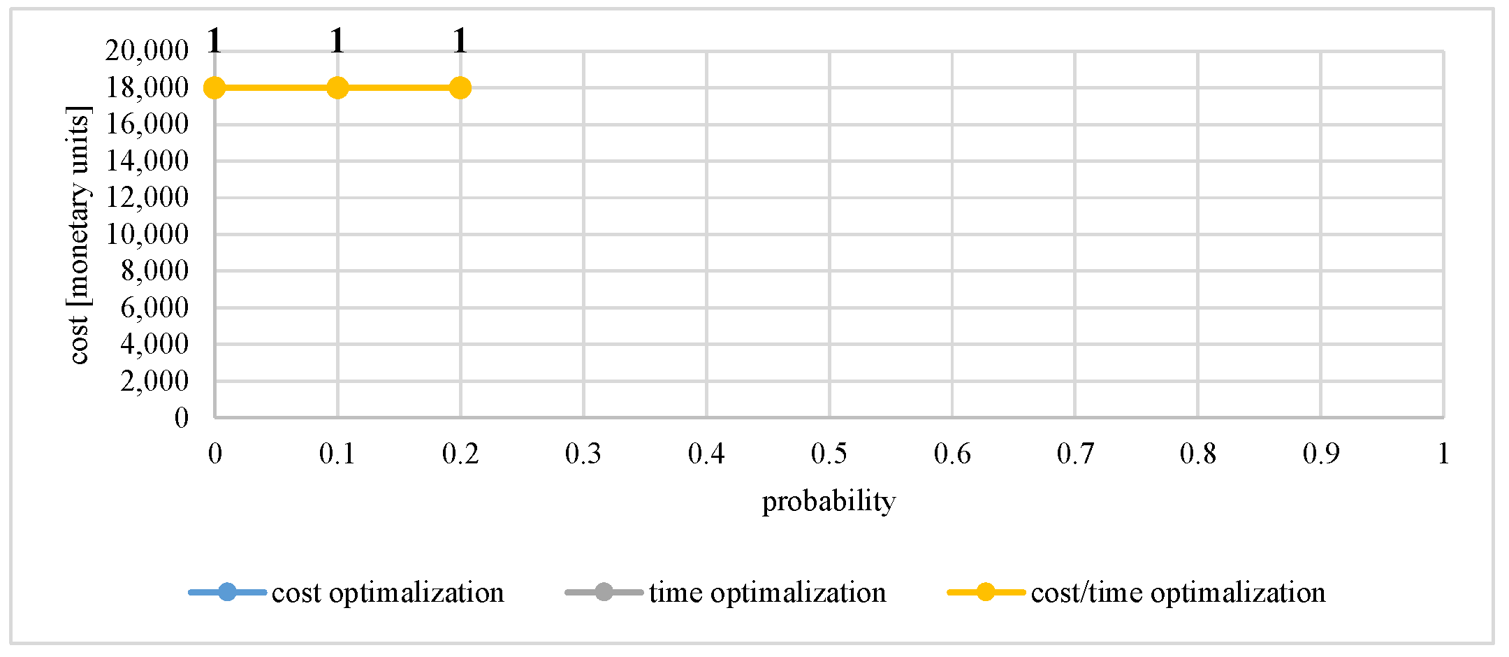
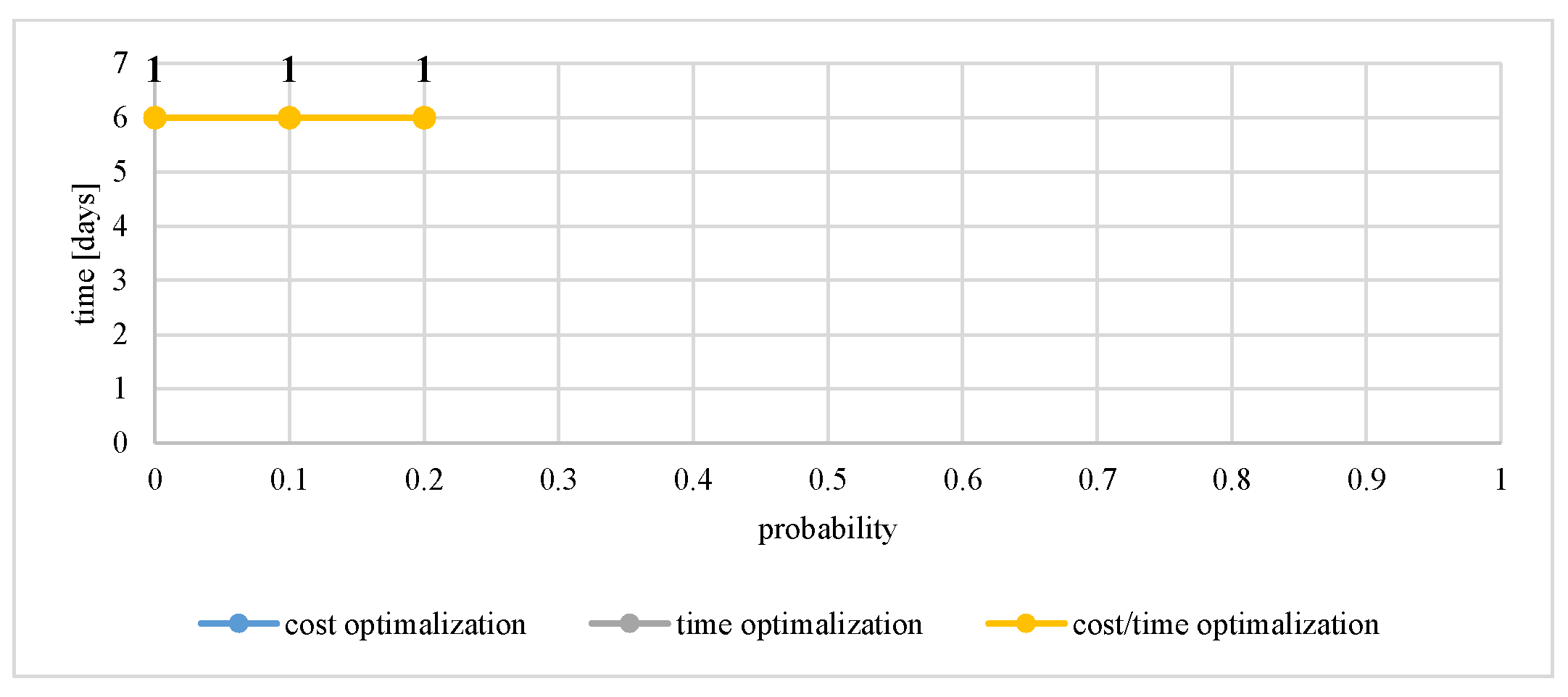
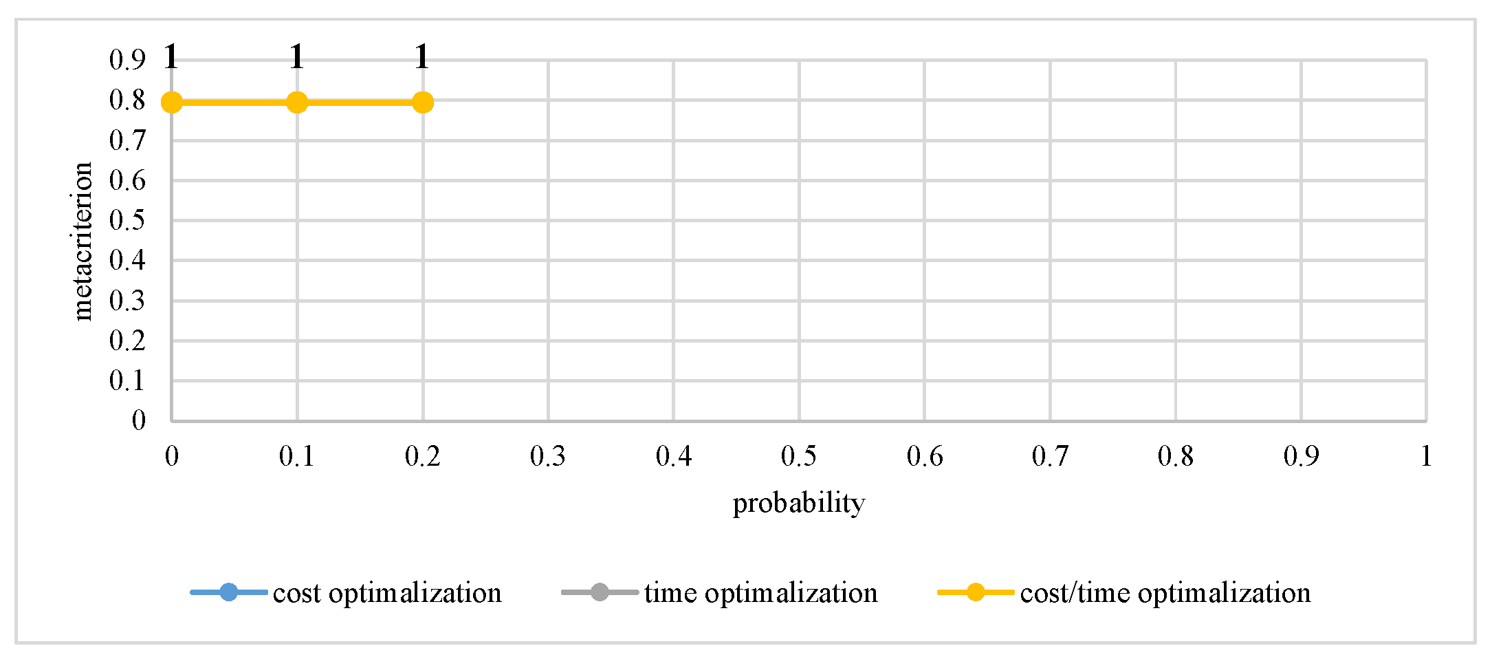
| Vertex 11 | >0 | 18,000.00 | 18,000.00 | 6.00 | 6.00 | 0.794872 | 0.794872 |
| ≥0.1 | 18,000.00 | 18,000.00 | solution not found | 6.00 | 0.794872 | 0.794872 | |
| ≥0.2 | 18,000.00 | 18,000.00 | 6.00 | 6.00 | 0.794872 | 0.794872 | |
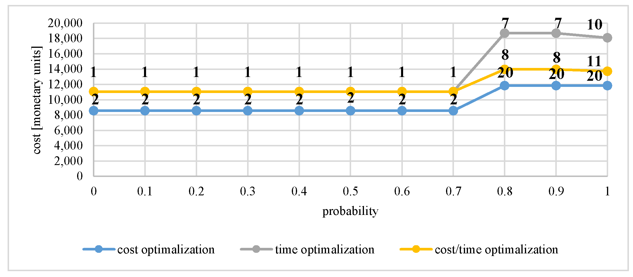
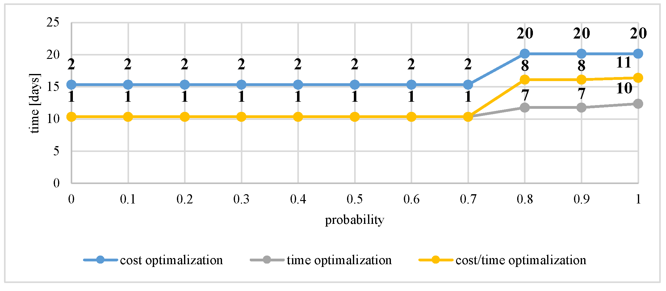
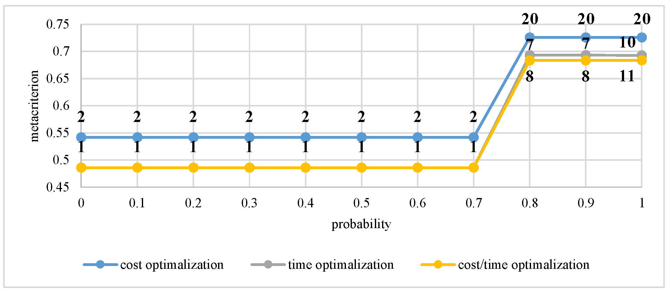
| Vertex 17 | >0 | 8555.56 | 8555.56 | 10.33 | 10.33 | 0.485979 | 0.485979 |
| ≥0.1 | 8555.56 | 8555.56 | 10.33 | 10.33 | 0.485979 | 0.485979 | |
| ≥0.2 | 8555.56 | 8555.56 | 10.33 | 10.33 | 0.485979 | 0.485979 | |
| ≥0.3 | solution not found * | 8555.56 | 10.33 | 10.33 | 0.485979 | 0.485979 | |
| ≥0.4 | 8555.56 | 8555.56 | solution not found * | 10.33 | 0.485979 | 0.485979 | |
| ≥0.5 | 8555.56 | 8555.56 | 10.33 | 10.33 | 0.485979 | 0.485979 | |
| ≥0.6 | solution not found * | 8555.56 | 10.33 | 10.33 | 0.485979 | 0.485979 | |
| ≥0.7 | 8555.56 | 8555.56 | 10.33 | 10.33 | 0.485979 | 0.485979 | |
| ≥0.8 | solution not found * | 11,841.67 | 12.37 | 11.78 | 0.683898 | 0.683426 | |
| ≥0.9 | 11,841.67 | 11,841.67 | 12.37 | 11.78 | 0.683898 | 0.683426 | |
| =1 | 11,841.67 | 11,841.67 | 12.37 | 12.37 | 0.683898 | 0.683898 | |
| Stochastic Network | Stochastic Decision Network | |||||
|---|---|---|---|---|---|---|
| No. of the Final Vertex | Probability of Being Carried Out | Expected Cost of Completion [Monetary Units] | Expected Completion Time [Days] | The optimal Expected Completion Cost [Monetary Units] | The Optimal Expected Completion Time [Days] | Metacriterion for the Weights: |
| 11 | 0.155 | 21290.32 | 9.58 | 18,000.00 for sub-networks: | 6.00 for sub-networks: | 0.795 for sub-networks: |
| 17 | 0.845 | 11891.62 | 14.85 | 11,841.00 for sub-networks: | 11.78 for sub-networks: | 0.683 for sub-networks: |
© 2019 by the authors. Licensee MDPI, Basel, Switzerland. This article is an open access article distributed under the terms and conditions of the Creative Commons Attribution (CC BY) license (http://creativecommons.org/licenses/by/4.0/).
Share and Cite
Śladowski, G.; Szewczyk, B.; Sroka, B.; Radziszewska-Zielina, E. Using Stochastic Decision Networks to Assess Costs and Completion Times of Refurbishment Work in Construction. Symmetry 2019, 11, 398. https://0-doi-org.brum.beds.ac.uk/10.3390/sym11030398
Śladowski G, Szewczyk B, Sroka B, Radziszewska-Zielina E. Using Stochastic Decision Networks to Assess Costs and Completion Times of Refurbishment Work in Construction. Symmetry. 2019; 11(3):398. https://0-doi-org.brum.beds.ac.uk/10.3390/sym11030398
Chicago/Turabian StyleŚladowski, Grzegorz, Bartłomiej Szewczyk, Bartłomiej Sroka, and Elżbieta Radziszewska-Zielina. 2019. "Using Stochastic Decision Networks to Assess Costs and Completion Times of Refurbishment Work in Construction" Symmetry 11, no. 3: 398. https://0-doi-org.brum.beds.ac.uk/10.3390/sym11030398