A Hybrid Model Based on a Two-Layer Decomposition Approach and an Optimized Neural Network for Chaotic Time Series Prediction

Abstract

The prediction of chaotic time series has been a popular research field in recent years. Due to the strong non-stationary and high complexity of the chaotic time series, it is difficult to directly analyze and predict depending on a single model, so the hybrid prediction model has become a promising and favorable alternative. In this paper, we put forward a novel hybrid model based on a two-layer decomposition approach and an optimized back propagation neural network (BPNN). The two-layer decomposition approach is proposed to obtain comprehensive information of the chaotic time series, which is composed of complete ensemble empirical mode decomposition with adaptive noise (CEEMDAN) and variational mode decomposition (VMD). The VMD algorithm is used for further decomposition of the high frequency subsequences obtained by CEEMDAN, after which the prediction performance is significantly improved. We then use the BPNN optimized by a firefly algorithm (FA) for prediction. The experimental results indicate that the two-layer decomposition approach is superior to other competing approaches in terms of four evaluation indexes in one-step and multi-step ahead predictions. The proposed hybrid model has a good prospect in the prediction of chaotic time series.

1. Introduction

Chaotic time series exist in a wide range of areas, such as nature, the economy, society, and industry. They contain many important and valuable information, useful for complex system modeling and prediction. Time series data mining is an important means of the control and decision-making of practical problems in various fields [1,2]. In recent years, scholars have carried out a great amount of research work on chaotic time series analysis and prediction. Han et al. [3] proposed an improved extreme learning machine combined with a hybrid variable selection algorithm for the prediction of multivariate chaotic time series, which can achieve high predictive accuracy and reliable performance. Chandra [4] put forward a competitive cooperative coevolution algorithm to train recurrent neural networks (RNNs) for chaotic time series prediction. Yaslan et al. [5] presented a hybrid model based on empirical mode decomposition (EMD) and support vector regression (SVR) for electricity load forecasting. Chen [6] proposed a prediction model of a radial basis function (RBF) neural network optimized by an artificial bee colony algorithm for prediction of traffic flow time series. A multilayered echo state machine with the addition of multiple layers of reservoirs was introduced in [7], and it could be more robust than the echo state network with a conventional reservoir in dealing with chaotic time series prediction.

The time series prediction models proposed in recent years are usually divided into three types: statistical models, artificial intelligence models, and hybrid models. The statistical models mainly include autoregressive (AR) models [8], the autoregressive moving average (ARMA), the autoregressive integrated moving average (ARIMA) [9], multivariate linear regression, the Gaussian process [10], and so on. Since statistical models require time series to be subject to certain a priori assumptions, such as stationarity, they are not ideal for practical systems with many uncertainties. With the development of computational intelligence, artificial intelligence models have obtained widespread attention. They are data-driven methods that do not require any a priori assumptions and thus have a wide range of applications. Commonly used artificial intelligence models include support vector regression [11], RBF neural networks [12], Elman neural networks [4], echo state networks [7], deep neural networks [13], extended Kalman filters [14], adaptive neuro-fuzzy inference systems (ANFISs) [15,16,17], etc. So as to improve the performance of single-model-based prediction models, a novel framework based on decomposition algorithm has been introduced for time series prediction [18]. Multiple decomposition methods have been put forward to analyze time series, thus forming the hybrid prediction models [19]. The subsequences obtained by the decomposition algorithms are much easier to predict than the original time series, which brings forward a new means of predicting nonlinear and non-stationary time series [20]. Ren et al. [21] introduced a hybrid model, EMD combined with kNN, for wind speed prediction. The model generated a set of feature vectors from the components obtained by EMD, and kNN was then employed for prediction. The suggested hybrid model performed well for long-term wind speed forecasting. An ensemble EMD (EEMD)–ARIMA model has been proposed to predict annual runoff time series [22]. According to the experimental results, it was concluded that the introduction of EEMD could observably improve prediction performance, and the EEMD–ARIMA model was superior to the ARIMA. It is confirmed that hybrid models perform better than their corresponding single models in chaotic time series prediction.

Though these existing hybrid prediction models have indeed increased the performance of chaotic time series prediction, they still cannot handle the chaotic time series with strong non-stationary and nonlinear very well. Hence, the hybrid models can be further improved to obtain more accurate predictions. For the sake of enhancing the accuracy of actual chaotic time series prediction, we put forward a novel hybrid model based on a two-layer decomposition technique and an optimized back propagation neural network (BPNN). The main contents and contributions of this paper are summarized as follows.

• A hybrid model based on a two-layer decomposition technique is proposed in this paper. For the sake of solving the problem that the prediction model based on single decomposition technique cannot completely deal with the nonlinear and non-stationary of chaotic time series, this paper puts forward a two-layer decomposition technique based on CEEMDAN and VMD, which is able to fully extract the complex characteristics of time series and improve prediction accuracy.
• A firefly algorithm (FA) is applied to optimize the weights between input and hidden layer, the weights between the hidden and output layer and the thresholds of neuron nodes, which can reduce the human interference of parameter settings and improve the function approximation ability of the neural network. A BPNN optimized by the FA is applied to predict the subsequences obtained by two-layer decomposition.
• The real world chaotic time series, daily maximum temperature time series in Melbourne, is used to assess the validity of the proposed hybrid model. The experimental results indicate that our hybrid model has a significant improvement in prediction accuracy compared to the existing single-model-based approaches and hybrid models based on the single layer decomposition technique.

The remainder of the paper is organized as follows. Preliminaries and related works are introduced in Section 2. In Section 3, we introduce the principles and the implementation steps of the proposed method. Section 4 presents the experiments illustrating the availability of the proposed model. Finally, conclusions and future directions are demonstrated in Section 5. For the convenience of reading, the notations used in this paper are shown in

Table 1. The notations used in this paper.

Notation	Meaning
$\epsilon (t)$	independent Gaussian white noise with unit variance
${\omega }_0$	a noise coefficient
$r_1\left(t\right)$	the first residue
$E_j(\cdot )$	a function to extract the j-th intrinsic mode function (IMF) decomposed by EMD
$u_k\left(t\right)$	the k-th mode of decomposition
${\omega }_k$	the center frequency of mode k
${\partial }_t(\cdot )$	partial derivative
$\sigma$	the Dirac distribution
$\ast$	convolution computation
$\alpha$	the balancing parameter of the data-fidelity constraint
$\lambda$	the Lagrangian multiplier
$\widehat{f}\left(\omega \right)$	the Fourier transforms of $f\left(t\right)$
$I_0$	the intensity of the light source
$\gamma$	the light absorption coefficient
$r_{ij}$	the distance between firefly $i$ and $j$
${\beta }_0$	the attractiveness at the light source $(r=0)$
$s_i$	the space positions of firefly $i$

.

2. Preliminaries and Related Works

In this section, we will firstly introduce the basic methods, including CEEMDAN, VMD, and the FA. Furthermore, related works of the hybrid prediction model will be described.

2.1. Complete Ensemble Empirical Mode Decomposition with Adaptive Noise

Ensemble EMD (EEMD) adds white noise to the original signal to solve the mode mixing problem of EMD. However, the white noise sequence cannot be absolutely canceled through the finite average, and the magnitude of reconstruction error depends on the times of integration. In addition, increasing the times of integration would lead to an increase computational burden. To solve these problems, CEEMDAN was proposed as an improved version of EEMD [23]. By adding a finite number of adaptive white noise at each stage, the CEEMDAN method is able to obtain the reconstruction error close to zero through a small average number of times of integration. Thus, CEEMDAN avoids the mode mixing problem in EMD, while reducing computational complexity compared to EEMD.

2.2. Variational Mode Decomposition

VMD is a novel non-recursive signal processing approach [24], which decomposes the original signal into a group of subsequences. Each subsequence is called a mode and is concentrated near a specific central pulsation frequency. For assessing the bandwidth of each mode, there are three main schemes: Firstly, apply the Hilbert transform to each mode separately, calculate the associated analytic signals, and then obtain a number of unilateral frequency spectrums. Then, adjust each mode to its estimated center frequency by adding an exponential term, so as to shift the frequency spectrums of these modes to the respective baseband. Finally, estimate the bandwidth of every mode by means of the Gaussian smoothness of the demodulated signal, for example, the L2-norm of the gradient.

2.3. Firefly Algorithm

The firefly algorithm (FA) [25] is a heuristic optimization algorithm based on firefly behavior, whereby flash signals are used to attract potential mates for positional movement. It is a swarm intelligence optimization algorithm and therefore has the advantages of a swarm intelligence algorithm. In addition, compared with other similar algorithms, it has the following two advantages. Firstly, it can realize automatic segmentation, which is well suited for solving highly nonlinear optimization problems. Secondly, the FA has multi-modal characteristics and can deal with multi-modal problems quickly and efficiently. The basic idea of the FA is to treat every point in space as a firefly, which is attracted to the brighter fireflies and moves in this direction. During the movement of the weakly glowing firefly, the position is updated until the optimal position is found. Since it is proposed, FA has been widely used to solve various practical problems.

2.4. Related Works

Aiming at the analysis of nonlinear and non-stationary time series, many hybrid models have been proposed. In [26], the EMD–BPNN is presented and applied to forecast tourism demand, namely the number of tourists. The hybrid model showed better performance than a single BPNN or ARIMA model. Zhou et al. [27] put forward a hybrid model of EEMD–GRNN (general regression neural network) for PM2.5 forecasting. Simulation results indicated that the EEMD–GRNN model outperformed the GRNN, multiple linear regression, and the ARIMA. This research was significant for the development of air quality warning systems. Moreover, a comparison work of hybrid prediction models based on wavelet decomposition, wavelet packet decomposition, EMD, and fast EEMD was implemented in [28]. The study investigated the decomposition and prediction performance of multiple hybrid models. In [29], VMD was adopted to decompose wind power time series into multiple modes, and Gram–Schmidt orthogonalization was used to eliminate redundant attributes. Next, the hybrid model based on VMD and extreme learning machines was proposed for short-term wind power forecasting. Similarly, Lahmiri [30] proposed a hybrid model for economic and financial time series forecasting, called VMD–GRNN. Jianwei E et al. [31] raised a hybrid model VMD–ICA–ARIMA for crude oil price forecasting. Wang et al. [32] suggested a hybrid model based on VMD, phase space reconstruction, and a wavelet neural network, which is reliable for multi-step prediction of wind speed time series.

As mentioned before, hybrid models based on decomposition methods, such as EMD, EEMD, and VMD, have been extensively used for time series modeling and have exhibited satisfactory performance.

3. Methodology

3.1. The Structure of CEEMDAN–VMD–FABP Model

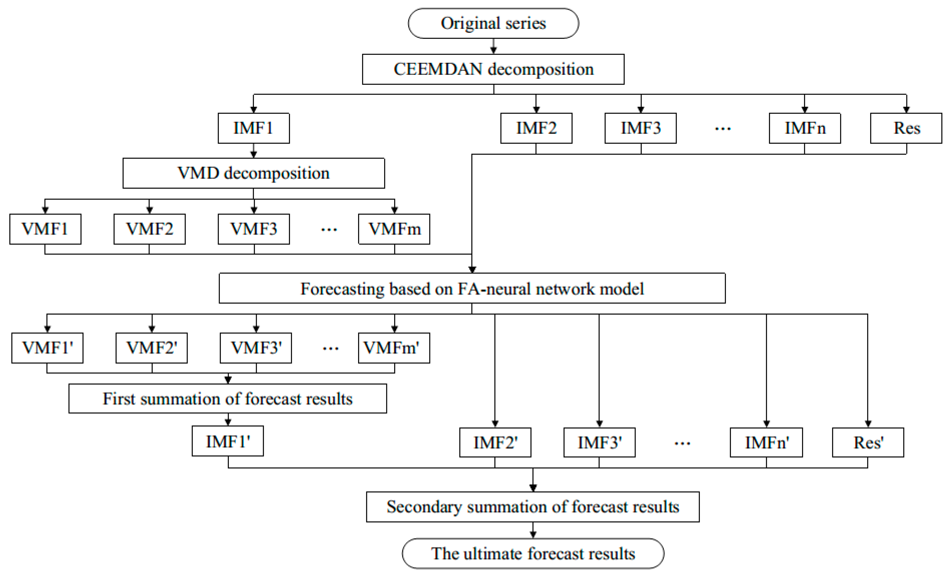
Subsequences obtained by an effective decomposition technique are much easier to analyze than an original time series, and a single-layer decomposition pattern is one of the most commonly adopted methods in existing hybrid models. Models based on a single-layer decomposition technique are able to increase the predictive performance of various chaotic time series to some extent, but they are difficult in completely reflecting the non-stationarity and irregularity of original signals. In view of this, we propose a novel two-layer decomposition approach using CEEMDAN and VMD for chaotic time series forecasting, which is shown in Figure 1. In addition, we adopt a BPNN optimized by an FA (FABP) to predict subsequences obtained by a two-layer decomposition operation. FABP has the ability to automatically optimize weights and thresholds, which is able to reduce the randomness of parameter selection and ultimately strengthen the function approximation ability of a neural network. Next, we will comprehensively introduce the structure of the proposed model.

The CEEMDAN method with noise robustness is first used to decompose the original signal. CEEMDAN has good performance in anti-noise, so the original signal is not denoised in this paper. At present, many scholars are committed to improving the CEEMDAN algorithm by increasing its robustness and improving its adaptive anti-noise performance so that it omits the process of denoising the original signal. Therefore, the original signal is automatically decomposed into a group of intrinsic mode functions (IMFs), namely IMF1, IMF2, …, IMFn, and a residue.

IMF1 has the highest frequency, which is the most difficult to track and predict. To improve the overall prediction accuracy of the original signal, the VMD algorithm is introduced here for the secondary decomposition of IMF1. IMF1 is decomposed by the VMD algorithm into VMF1, VMF2, …, VMFm. Next, they are each predicted by FABP. Afterwards, the prediction results of these subsequences are combined into the final result of IMF1. Furthermore, the subsequences IMF2, …, IMFn and the residue are each predicted using FABP. The summation of the prediction results of IMF2, …, IMFn and the residue is superimposed with the prediction result of the IMF1. The final forecast result of the original chaotic signal is obtained. At this point, the entire forecast process is complete.

3.2. Algorithm Design

3.2.1. CEEMDAN for Original Time Series

First, the CEEMDAN decomposition algorithm [23] is adopted to obtain a group of IMFs adaptively. The computational process of CEEMDAN is as follows.

Step 1. A collection of noise-added original time series is created: $x^i\left(t\right)=x\left(t\right)+{\omega }_0{\epsilon }^i\left(t\right)$, $i\in \{1,\dots ,I\}$, where $\epsilon (t)$ is independent Gaussian white noise with unit variance, and ${\omega }_0$ is a noise coefficient.

Step 2. For each $x^i\left(t\right)$, EMD is used to obtain the first IMF and take the average:

$$c_1\left(t\right)=\frac{1}{I}{\displaystyle \sum _{i=1}^I{c}_1^i\left(t\right)}.$$

(1)

The first residue is then $r_1\left(t\right)=x\left(t\right)-c_1\left(t\right)$.

Essentially, the procedure of the EMD algorithm is a sifting process from which IMFs can be obtained [33]. The specific computation process of the signal $x^i(t)$ is described as follows. Firstly, we obtain every local maxima and local minima of $x^i(t)$. Next, the upper envelope $u(t)$ and the lower envelope $l(t)$ are structured by cubic spline interpolation. Finally, we calculate the average of $u(t)$ and $l(t)$ and record the average as $m(t)$.

$$m\left(t\right)=\left(u\left(t\right)+l\left(t\right)\right)/2.$$

(2)

We subtract $m(t)$ from the original signal $x^i(t)$ and record the result as $c_1^i(t)$.

$$c_1^i\left(t\right)=x^i\left(t\right)-m\left(t\right).$$

(3)

It is then determined whether $c_1^i(t)$ is an integral part of the IMF by checking whether $c_1^i(t)$ satisfies the above two conditions. The IMFs should conform to the following two conditions: (1) the absolute value of the difference between the number of extreme points and zero crossing must be less than or equal to 1 in the whole data series; (2) the average of the upper envelope and lower envelope must be zero at any point. If $c_1^i(t)$ meets the above two conditions, $c_1^i(t)$ is recognized as IMF1. In the meantime, $r(t)=x(t)-c(t)$ is used as the residue instead of $x(t)$. If $c_1^i(t)$ is not an IMF, $c_1^i(t)$ is used instead of $x^i(t)$, and the above process is repeated until we IMF1 is obtained.

Step 3. The second IMFs is obtained by decomposing the noise-added residue $r_1+{\omega }_1{E}_1\left({\epsilon }_1\left(t\right)\right)$:

$$c_2\left(t\right)=\frac{1}{I}{\displaystyle \sum _{i=1}^I{E}_1\left(r_1+{\omega }_1{E}_1\left({\epsilon }^i\left(t\right)\right)\right)},$$

(4)

where $E_j(\cdot )$ represents the j-th IMF obtained by EMD.

Step 4. The remaining IMFs are repeated until the number of extreme points of the residual signal does not exceed two.

So far, the original signal has been decomposed into a series of IMF components, namely IMF1, IMF2, …, IMFn. Due to the highest frequency and unpredictability of IMF1, this research introduces the second decomposition of the IMF1 based on the VMD.

3.2.2. VMD for IMF1

The main task of the VMD algorithm [34] is to solve the following constrained optimization problem:

$$\begin{array}{l}\underset{\left\{u_k\right\},\left\{{\omega }_k\right\}}{\min }{\displaystyle \sum _k{\Vert {\partial }_t\left[\left(\sigma \left(t\right)+\frac{j}{\pi t}\right)\ast u_k\left(t\right)\right]e^{-j{\omega }_{k}t}\Vert }_2^2}\\ s.t.\hspace{0.17em}\hspace{0.17em}\hspace{0.17em}\hspace{0.17em}\hspace{0.17em}{\displaystyle \sum _k{u}_k=f}\end{array}$$

(5)

where $u_k\left(t\right)$ denotes the k-th mode of decomposition, ${\omega }_k$ is the center frequency of mode $k$, ${\partial }_t(\cdot )$ denotes partial derivative, $\sigma$ indicates the Dirac distribution, $\ast$ denotes convolution computation, and f is the original signal to be decomposed.

In order to solve the above constrained optimization problem, a quadratic penalty term and a Lagrangian multiplier are shown in Equation (6). The former is conducive to enforcing the constraint, and the latter helps to improve convergence. Hence, the translated unconstrained form is shown as

$$L\left(\left\{u_k\right\},\left\{{\omega }_k\right\},\lambda \right)=\alpha {\displaystyle \sum _k{\Vert {\partial }_t\left[\left(\sigma \left(t\right)+\frac{j}{\pi t}\right)\ast u_k\left(t\right)\right]e^{-j{\omega }_{k}t}\Vert }_2^2}+{\Vert f-{\displaystyle \sum _k{u}_k\left(t\right)}\Vert }_2^2+\langle \lambda \left(t\right),f\left(t\right)-{\displaystyle \sum _k{u}_k\left(t\right)}\rangle ,$$

(6)

where $\alpha$ represents the balancing parameter, and $\lambda$ is the Lagrangian multiplier.

An alternate direction method of multipliers (ADMM) [35] is applied to settle the optimization problem of (6). The saddle point of the obtained augmented Lagrangian $L$ in iterative optimization process is determined by AMDD. The suboptimized solution is embedded into ADMM and optimized in the Fourier domain. The detailed calculation process can be found in [24]. To implement the VMD algorithm and update the modes, $u_k$ and ${\omega }_k$ are iterated in two directions according to the following solutions:

$$u_k^{n+1}=\arg \min \{\alpha {\displaystyle \sum _k{\Vert {\partial }_t\left[\left(\sigma \left(t\right)+\frac{j}{\pi t}\right)\ast u_k\left(t\right)\right]e^{-j{\omega }_{k}t}\Vert }_2^2}+{\Vert f-{\displaystyle \sum _k{u}_i\left(t\right)-\frac{\lambda \left(t\right)}{2}}\Vert }_2^2,$$

(7)

$${\omega }_k^{n+1}=\arg \min {\Vert {\partial }_t\left[\left(\sigma \left(t\right)+\frac{j}{\pi t}\right)\ast u_k\left(t\right)\right]e^{-j{\omega }_{k}t}\Vert }_2^2.$$

(8)

Subsequently, the solutions are represented as follows:

$${\widehat{u}}_k^{n+1}\left(\omega \right)=\frac{\widehat{f}\left(\omega \right)-{\displaystyle \sum _{i\ne k}{\widehat{u}}_i\left(\omega \right)+\frac{\widehat{\lambda }\left(\omega \right)}{2}}}{1+2\alpha {\left(\omega -{\omega }_k\right)}^2}$$

(9)

$${\omega }_k^{n+1}=\frac{{\displaystyle {\int }_0^{\infty }\omega {\left|{\widehat{u}}_k\left(\omega \right)\right|}^{2}d\omega }}{{\displaystyle {\int }_0^{\infty }{\left|{\widehat{u}}_k\left(\omega \right)\right|}^{2}d\omega }}$$

(10)

where $\widehat{f}\left(\omega \right)$, ${\widehat{u}}_k\left(\omega \right)$, and $\widehat{\lambda }\left(\omega \right)$ represent the Fourier transforms of $f\left(t\right)$, $u_k\left(t\right)$, and $\lambda \left(t\right)$, and n denotes the number of iterations.

The complete calculation process of VMD is organized in Algorithm 1. IMF1 is decomposed by VMD algorithm into VMF1, VMF2, …, VMFm.

Algorithm 1: ADMM Optimization Process for VMD

Initialize$\left\{{\widehat{u}}_k^1\right\}$, $\left\{{\omega }_k^1\right\}$, ${\widehat{\lambda }}^1$, $n=0$

repeat

$n=n+1$

for $k=1:K$ do

Update ${\widehat{u}}_k^1$ for all $\omega \ge 0$

${\widehat{u}}_k^{n+1}\left(\omega \right)=\frac{\widehat{f}\left(\omega \right)-{\displaystyle \sum _{i\ne k}{\widehat{u}}_i\left(\omega \right)+\frac{\widehat{\lambda }\left(\omega \right)}{2}}}{1+2\alpha {\left(\omega -{\omega }_k\right)}^2}$

Update ${\omega }_k$

${\omega }_k^{n+1}=\frac{{\displaystyle {\int }_0^{\infty }\omega {\left|{\widehat{u}}_k\left(\omega \right)\right|}^{2}d\omega }}{{\displaystyle {\int }_0^{\infty }{\left|{\widehat{u}}_k\left(\omega \right)\right|}^{2}d\omega }}$

end for

for all $\omega \ge 0$

${\widehat{\lambda }}^{n+1}\left(\omega \right)\leftarrow {\widehat{\lambda }}^n\left(\omega \right)+\gamma \left[\widehat{f}\left(\omega \right)-{\displaystyle \sum _k{\widehat{u}}_k^{n+1}\left(\omega \right)}\right]$

until convergence ${\displaystyle {\sum }_k\Vert {\widehat{u}}_k^{n+1}-{\widehat{u}}_k^n\Vert {}_2^2/{\Vert {\widehat{u}}_k^n\Vert }_2^2}<\epsilon$

3.2.3. BPNN Optimized by a Firefly Algorithm

After two-layer decomposition, a BPNN is used to predict all subsequences obtained by decomposition. The FA is adopted to optimize the parameters of the BPNN and is capable of improving the BPNN’s function approximation ability.

The search process is related to two important parameters of fireflies: the brightness and mutual attraction of the fireflies. Bright fireflies will attract the weak fireflies to move to them. The brighter the lights are, the better their positions are, and the brightest fireflies represent the optimal solution of the function. The higher a firefly’s brightness is, the more attractive it is to other fireflies. If the luminance is the same, the fireflies will engage in a random motion, and the two important parameters are inversely proportional to the distance. The greater the distance is, the smaller the attraction is.

The relative fluorescent brightness of a firefly is defined as

$$I=I_0{e}^{-\gamma r_{ij}{}^2},$$

(11)

where $I_0$ denotes the intensity of the light source. The better the objective function value is, the higher the firefly’s brightness is. $\gamma$ represents the light absorption coefficient. As the distance increases and the transmission medium weakens the light intensity, the fluorescence gradually decreases. The light absorption coefficient is set to reflect this characteristic. The parameter $r_{ij}$ denotes the distance between firefly $i$ and $j$, which is calculated according to the following formula:

$$r_{ij}=\sqrt{{\displaystyle \sum _{k=1}^n{\left(s_{ik}-s_{jk}\right)}^2}},$$

(12)

where $n$ represents the dimension of the problem.

Once a firefly is attracted by the flash of other fireflies, the attractiveness $\beta$ is updated based on

$$\beta ={\beta }_0{e}^{-\gamma r_{ij}{}^2},$$

(13)

where ${\beta }_0$ denotes the attractiveness at the light source $(r=0)$.

The formula for updating the location of fireflies is as follows:

$$s_i\left(t+1\right)=s_i\left(t\right)+{\beta }_0{e}^{-\gamma r_{ij}{}^2}\left(s_j\left(t\right)-s_i\left(t\right)\right)+\alpha \epsilon ,$$

(14)

where $s_i$ and $s_j$ denotes the space positions of firefly $i$ and $j$, separately. $\alpha$ denotes the step factor, and $\epsilon$ represents a random value.

The main algorithm process of the FA can be described as Algorithm 2.

Algorithm 2: Process of the Firefly Algorithm

Initialize$n$, ${\beta }_0$, $\gamma$, $\alpha$, $\epsilon$, $t=0$

Define the maximum number of iterations (MaxGeneration).

while$t<MaxGeneration$

$t=t+1$

for $i=1:n$

for $j=1:i$

Calculate light intensity $I_i$ at $s_i$ position.

If $I_j>I_i$

Move firefly $i$ towards $j$.

end if

Update the attractiveness values.

Evaluate the new solutions and update the light intensity.

end for

end for

Rank the fireflies and find the current best.

end while

Output the global optimal value.

We then obtain all prediction results of all subsequence, and the final prediction results of all sub-signals obtained by decomposition are superimposed. The advantages of this approach are verified in the next section.

4. Experimental Results

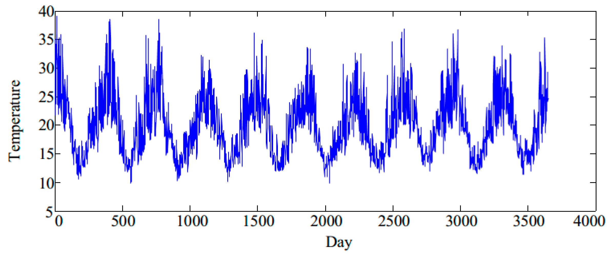
In this section, the daily maximum temperature time series in Melbourne is applied to analyze and verify the availability of the presented method. The experimental data is collected from the real world. The evaluation criteria are selected as root-mean-squared error (RMSE), normalized root-mean-square error (NRMSE), mean absolute percentage error (MAPE), and symmetric mean absolute percentage error (SMAPE). All prediction errors shown next are the mean values of 50 experimental results. The expressions are as follows:

$$\mathrm{RMSE}={\left[\frac{1}{n-1}{\displaystyle \sum _{k=1}^n{\left[\widehat{y}\left(k\right)-y\left(k\right)\right]}^2}\right]}^{\raisebox{1ex}{$1$}\!\left/ \!\raisebox{-1ex}{$2$}\right.},$$

(15)

$$\mathrm{NRMSE}=\frac{{\left[\frac{1}{n-1}{\displaystyle \sum _{k=1}^n{\left[\widehat{y}\left(k\right)-y\left(k\right)\right]}^2}\right]}^{\raisebox{1ex}{$1$}\!\left/ \!\raisebox{-1ex}{$2$}\right.}}{y_{\max }-y_{\min }},$$

(16)

$$\mathrm{MAPE}=\frac{100}{n}{\displaystyle \sum _{k=1}^n\left|\frac{\widehat{y}\left(k\right)-y\left(k\right)}{y\left(k\right)}\right|},$$

(17)

$$\mathrm{SMAPE}=\frac{1}{n}{\displaystyle \sum _{k=1}^n\frac{\left|y\left(k\right)-\widehat{y}\left(k\right)\right|}{\left|y\left(k\right)\right|+\left|\widehat{y}\left(k\right)\right|}},$$

(18)

where $y(k)$ denotes the real value, $\widehat{y}(k)$ denotes the predicted value, and $n$ denotes the number of samples.

The daily maximum temperature time series in Melbourne is used in the experiment. The dataset contains the daily maximum temperature from 3 January 1981 to 31 December 31 1990, a total of 3650 samples, which is shown in Figure 2. The training set is made up of the first 3000 samples, and the testing set is composed of the remaining 650. In order to compare the effectiveness of the model, six other methods were used in the comparative experiments: an RBF neural network, [36], an ANFIS [37], the original BP model, FABP, FABP with CEEMDAN decomposition (CEEMDAN–FABP), and FABP with VMD decomposition (VMD–FABP). The experimental environment involved the Windows 7 operating system, and all experiments were carried out using MATLAB R2016a on a 3.50 GHz, Intel(R) Core i3-4150M CPU with 6 GB RAM.

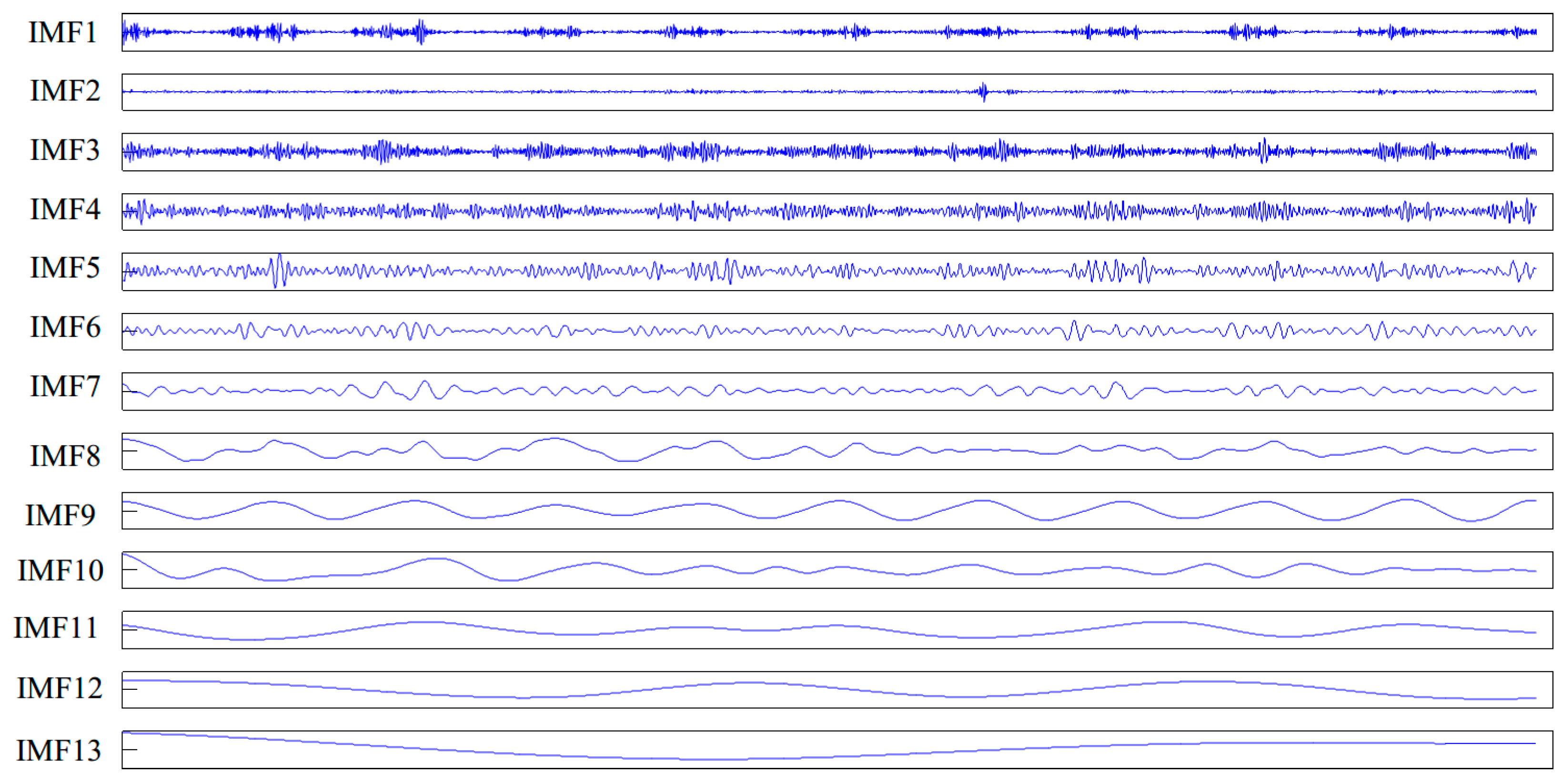
Figure 3 shows the decomposition results of the original time series based on CEEMDAN, which adaptively obtains 13 IMFs. CEEMDAN has good anti-noise performance, so this paper leaves out the de-noising process of the original time series.

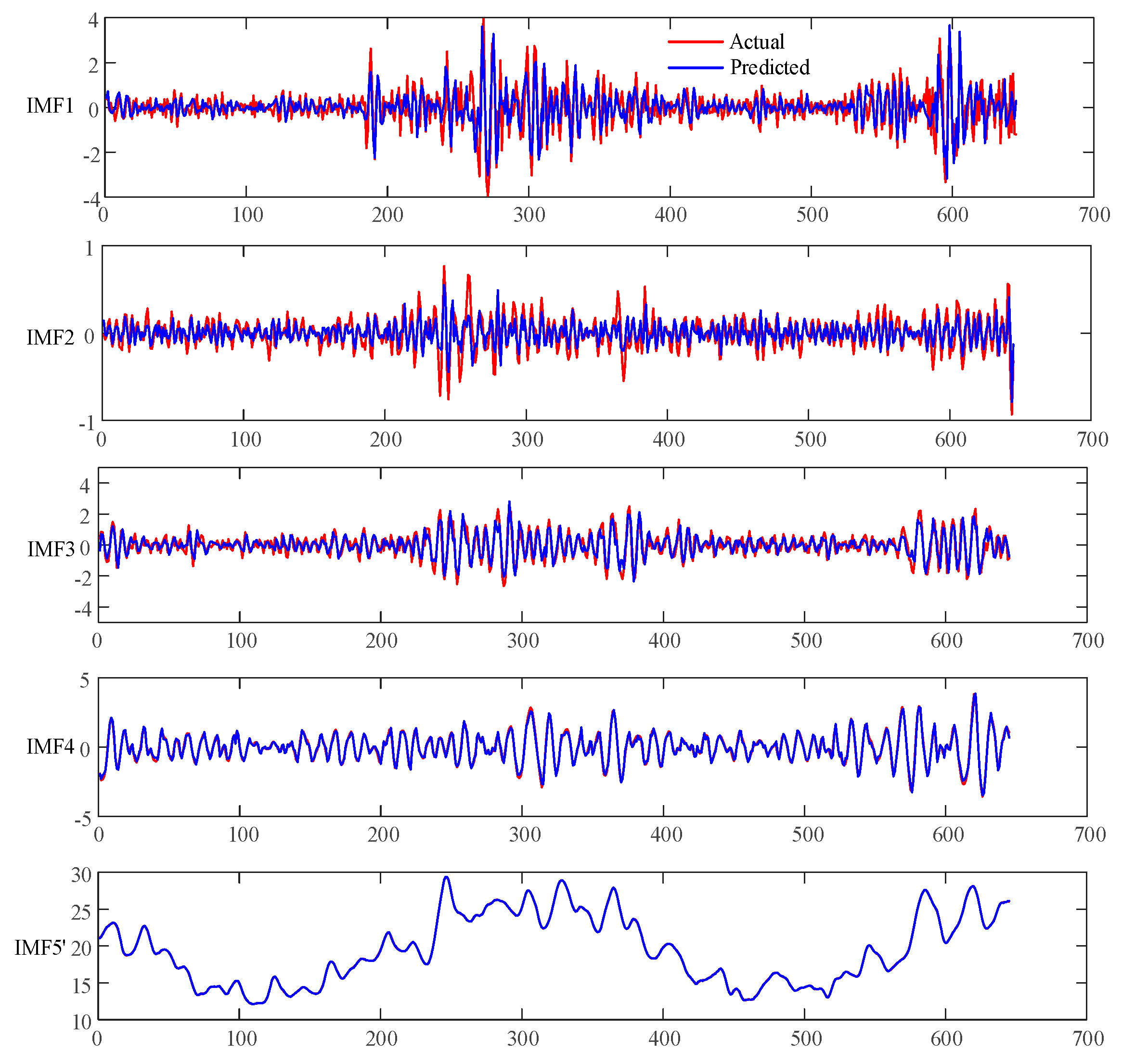
In this paper, sample entropy is an indicator for judging the way IMF predicts. Figure 4 shows the sample entropies of the IMFs. The entropy of the original time series is 0.81, which is indicated by the dotted line. In this research, the IMF components, whose entropy is greater than the entropy of the original time series, are predicted separately, because these IMFs are highly complex. The IMFs whose entropies are smaller than the original time series are combined and superimposed. After the combined operation, the model complexity and computational time are significantly reduced, while ensuring accuracy of prediction. Based on the results in Figure 4, the first four IMF components should be predicted separately, while the IMF components from 5 to 13 should be combined for prediction.

We obtained the prediction results of five IMF components, as shown in Figure 5. It can be observed that the prediction curve of each IMF is able to track the actual values, and the prediction trend is basically consistent. Due to the high frequency characteristics of IMF1, accurate prediction and tracking is more difficult, resulting in larger prediction errors for IMF1.

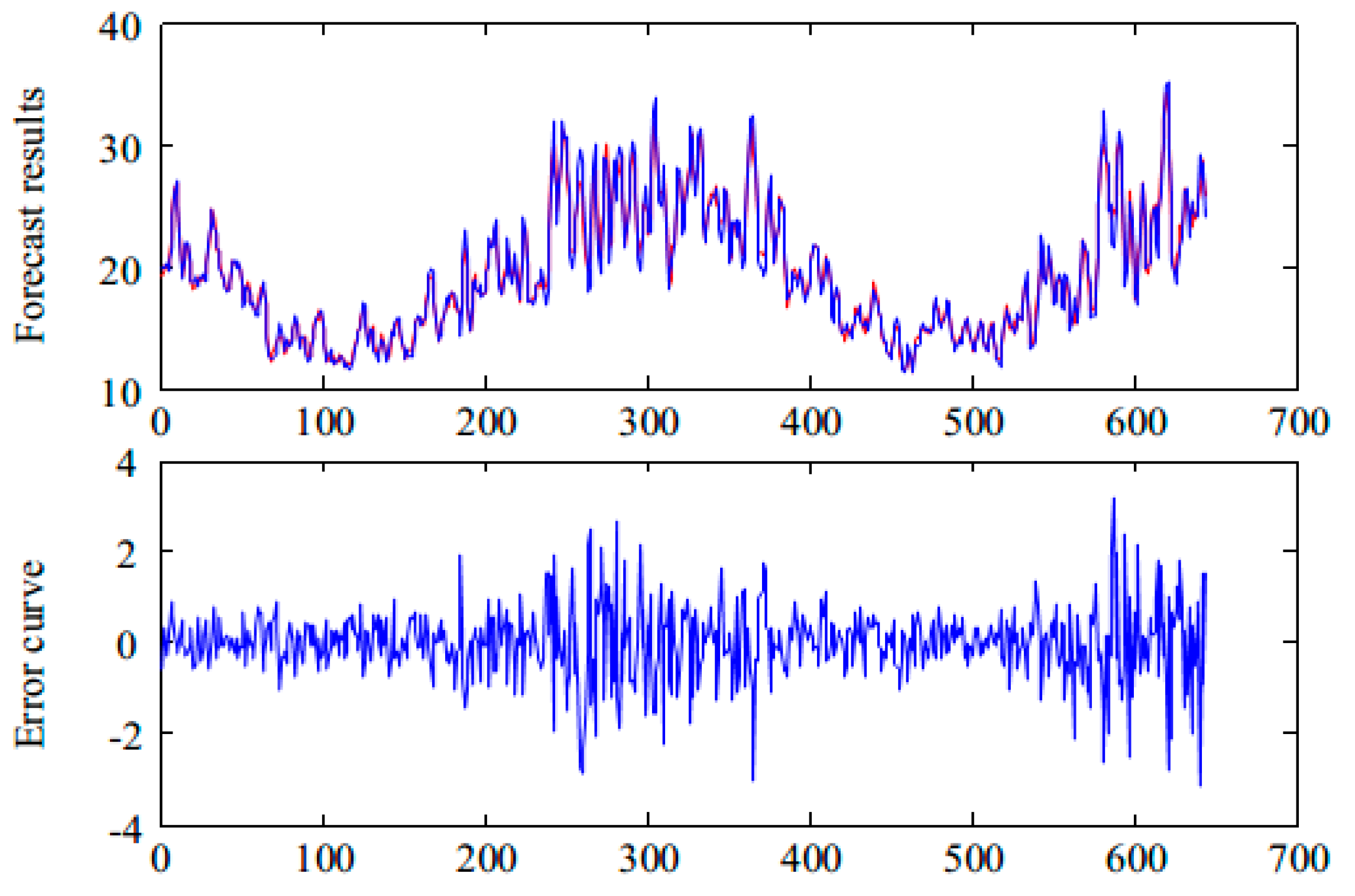
Figure 6 shows the final prediction results of the hybrid model of CEEMDAN and FABP. It can be seen that the prediction curve can track the real curve well and that the prediction error is small. The prediction result can be obtained in the case of the original time series without denoising.

The prediction errors presented in Figure 5 and Figure 6 are shown in

Table 2. Overall prediction error and prediction error of IMF1.

Prediction Error	RMSE	NRMSE	MAPE	SMAPE
Overall prediction error	0.7763	0.0325	0.0277	0.0138
IMF1 prediction error	0.6361	0.0808	1.8515	0.5829

. As can be seen from Table 2, the overall prediction error of the time series is 0.7763, while the prediction error of IMF1 is 0.6361. Therefore, if the prediction accuracy of IMF1 can be improved, the overall prediction accuracy will be greatly improved. Based on the above analysis, we propose the application of a two-layer decomposition strategy to further decompose the IMF1 component.

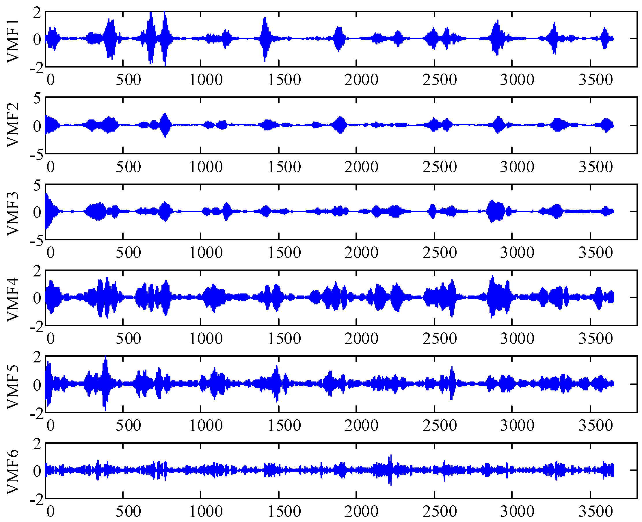
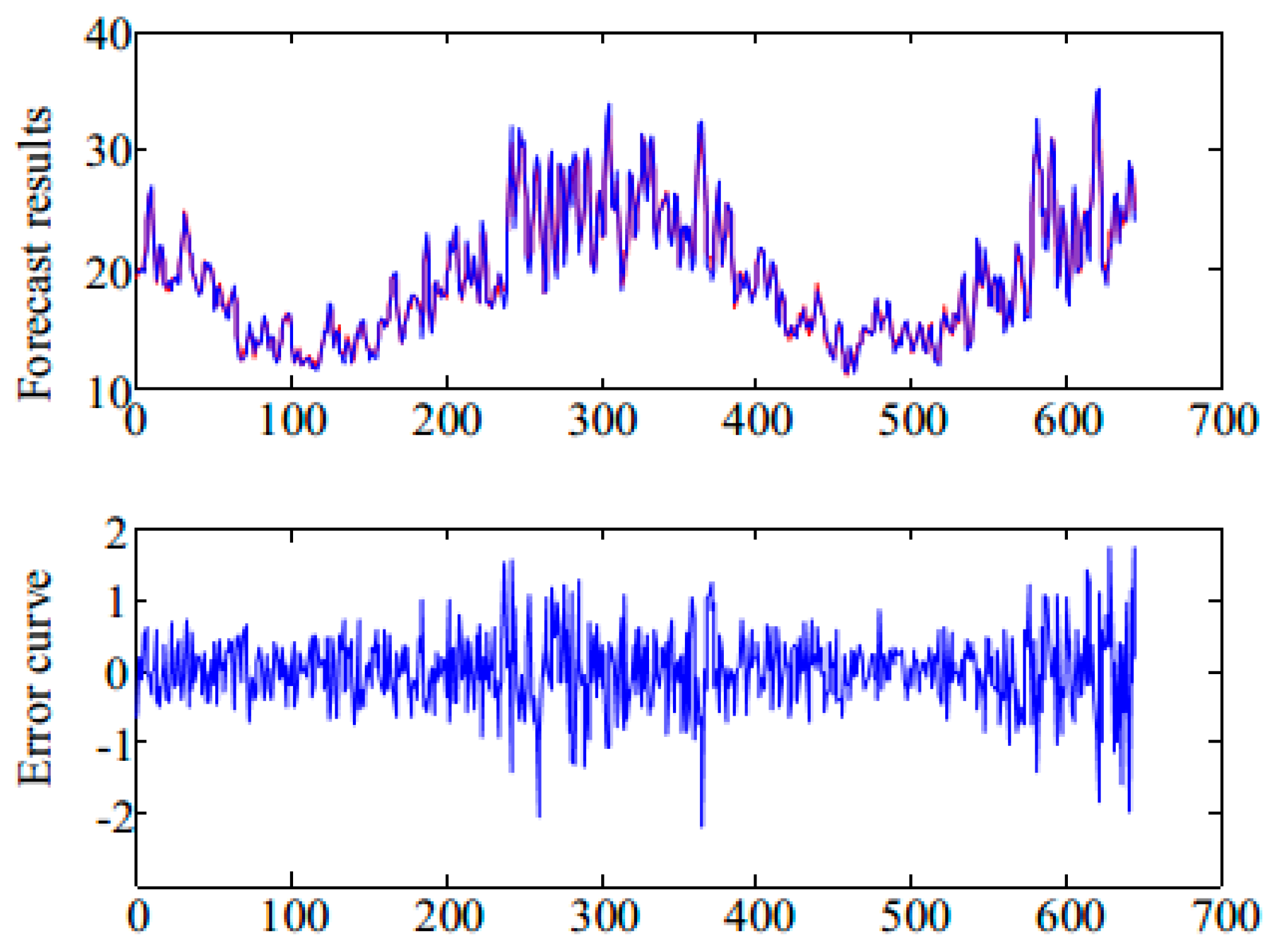
The IMF1 component is decomposed into six subsequences based on the VMD algorithm. The decomposition results of the IMF1 component are shown in Figure 7. We use FABP to predict VMF1, …, VMF6, and we combine the prediction results to obtain the prediction results of the IMF1 component. Next, we combine the prediction results of IMF1 with IMF2, …, IMF5’ components, thereby obtaining the prediction results of daily maximum temperature time series in Melbourne, which are shown in Figure 8. The error indexes of different prediction models are shown in

Table 3. Prediction errors of daily maximum temperature time series based on different algorithms (one step ahead).

Model	RMSE	NRMSE	MAPE	SMAPE	Training Time	Testing Time
RBF	1.7241	0.0721	0.0695	0.0345	0.9984	0.1092
ANFIS	3.2410	0.1356	0.1224	0.0598	22.3393	0.0936
BP	1.3818	0.0578	0.0511	0.0255	0.4368	0.0468
FABP	1.3618	0.0570	0.0505	0.0251	34.4294	0.0780
CEEMDAN–FABP	0.7763	0.0325	0.0277	0.0138	151.3834	0.1404
VMD–FABP	0.7026	0.0294	0.0266	0.0132	197.1852	0.2340
CEEMDAN–VMD–FABP	0.5131	0.0215	0.0198	0.0099	307.5092	0.2964

. It can be seen that the proposed two-layer decomposition algorithm can significantly reduce the prediction error and improve prediction accuracy compared with the direct prediction. This is mainly because the decomposition algorithm converts complex original signals into several simple and easy-to-analyze sub-signals, which is conducive to analysis and prediction. Based on the two-layer decomposition model, the prediction error is smaller than the single-layer approach, and the prediction performance is improved.

We conducted one-step-, two-step-, three-step-, and five-step-ahead prediction experiments on the time series. The corresponding prediction errors, including RMSE, NRMSE, MAPE, and SMAPE, are shown in Table 3,

Table 4. Prediction errors of daily maximum temperature time series based on different algorithms (two steps ahead).

Model	RMSE	NRMSE	MAPE	SMAPE
RBF	2.6741	0.1119	0.1051	0.0517
ANFIS	3.4725	0.1453	0.1317	0.0644
BP	2.4105	0.1009	0.0912	0.0454
FABP	2.4032	0.1006	0.0924	0.0456
CEEMDAN–FABP	0.9292	0.0389	0.0346	0.0172
VMD–FABP	0.7240	0.0303	0.0276	0.0138
CEEMDAN–VMD–FABP	0.6910	0.0289	0.0262	0.0130

,

Table 5. Prediction errors of daily maximum temperature time series based on different algorithms (three steps ahead).

Model	RMSE	NRMSE	MAPE	SMAPE
RBF	3.3242	0.1391	0.1286	0.0628
ANFIS	3.4715	0.1453	0.1330	0.0651
BP	3.1497	0.1318	0.1211	0.0589
FABP	3.1435	0.1315	0.1194	0.0587
CEEMDAN–FABP	1.1266	0.0471	0.0420	0.0209
VMD–FABP	0.9105	0.0381	0.0345	0.0172
CEEMDAN–VMD–FABP	0.8692	0.0364	0.0333	0.0166

and

Table 6. Prediction errors of daily maximum temperature time series based on different algorithms (five steps ahead).

Model	RMSE	NRMSE	MAPE	SMAPE
RBF	3.4960	0.1463	0.1353	0.0662
ANFIS	3.4408	0.1440	0.1333	0.0654
BP	3.3497	0.1402	0.1295	0.0633
FABP	3.3595	0.1406	0.1285	0.0632
CEEMDAN–FABP	1.5822	0.0662	0.0598	0.0297
VMD–FABP	1.2500	0.0523	0.0487	0.0242
CEEMDAN–VMD–FABP	0.9864	0.0413	0.0370	0.0183

. According to the results presented in the tables, the proposed model has a minimum prediction error in multiple prediction experiments, which indicates that the hybrid model of CEEMDAN–VMD–FABP has the best prediction performance. We can also say that the hybrid model based on the two-layer decomposition approach is better than the hybrid models based on a single decomposition approach. Surprisingly, although the ANFIS performed poorly in one-step prediction, its one-step prediction and multi-step prediction have similar effects, especially in the five-step ahead prediction experiment, and its performance is better than the RBF in multi-step prediction. The ANFIS method shows stability ability in terms of prediction, although the overall effect was not satisfactory. The prediction results of other models except for the ANFIS basically conform to the actual law. The more advanced the steps are, the more difficult it is to predict the chaotic time series.

To show the above experimental results more intuitively, we transform the error values, i.e. the RMSE, NRMSE, MAPE, and SMAPE shown in Table 3, Table 4, Table 5 and Table 6, into a column chart, presented in Figure 9. It can be seen that the proposed hybrid model of CEEMDAN–VMD–FABP has the best performance. The proposed two-layer decomposition model has minimum prediction error in one-step-, two-step-, three-step-, and five-step-ahead prediction.

Moreover, we compared the training time and testing time in one-step-ahead prediction. Under different prediction steps, the running time is not much different, so we only list the running time of one-step prediction in Table 3. As can be seen in the table, the testing time of each method is not much different. Although the method proposed in this paper has the longest training time, the experimental results prove that the proposed two-layer decomposition model can obtain the best prediction accuracy, which shows the effectiveness of the proposed method. Moreover, even if the training time is long, the overall running time is only a few minutes (not long), completely within the acceptable range.

5. Conclusions

In this paper, we propose a two-layer decomposition technique consisting of CEEMEAN and VMD. We obtained a group of subsequences by a two-layer decomposition method. These subsequences were separately predicted, and the prediction results were combined to obtain the final result. For the prediction, we used a BPNN optimized by a firefly algorithm. From this work, the following can be concluded:

• The actual time series is usually non-stationary and noisy. It is generally difficult to analyze the original time series. CEEMDAN is an anti-noise decomposition method, and VMD can handle non-stationary signals very well. Therefore, subsequences decomposed by CEEMDAN and VMD are easy to analyze and predict.
• After decomposition of the original signal, the BPNN was used for prediction. At this stage, the parameters in the BPNN greatly influenced prediction accuracy. Therefore, in order to reasonably select the model parameters, the FA algorithm was introduced to optimize the parameters of BP.

In general, in order to improve prediction accuracy, the following can be considered for further study: Firstly, original input variables were analyzed to eliminate factors that are not conducive to analysis and prediction. Secondly, we optimized the prediction model at the prediction stage. We studied the two aspects simultaneously, and the experimental results demonstrate the effectiveness of the proposed method.

References

- Shah, H.; Tairan, N.; Garg, H.; Ghazali, R. A Quick Gbest Guided Artificial Bee Colony Algorithm for Stock Market Prices Prediction. Symmetry 2018, 10, 292. [Google Scholar] [CrossRef]
- Zhai, H.; Cui, L.; Nie, Y.; Xu, X.; Zhang, W. A Comprehensive Comparative Analysis of the Basic Theory of the Short Term Bus Passenger Flow Prediction. Symmetry 2018, 10, 369. [Google Scholar] [CrossRef]
- Han, M.; Zhang, R.; Xu, M. Multivariate Chaotic Time Series Prediction Based on ELM–PLSR and Hybrid Variable Selection Algorithm. Neural Process. Lett. 2017, 46, 705–717. [Google Scholar] [CrossRef]
- Chandra, R. Competition and collaboration in cooperative coevolution of Elman recurrent neural networks for time-series prediction. IEEE Trans. Neural Netw. Learn. Syst. 2015, 26, 3123–3136. [Google Scholar] [CrossRef] [PubMed]
- Yaslan, Y.; Bican, B. Empirical mode decomposition based denoising method with support vector regression for time series prediction: A case study for electricity load forecasting. Measurement 2017, 103, 52–61. [Google Scholar] [CrossRef]
- Chen, D. Research on traffic flow prediction in the big data environment based on the improved RBF neural network. IEEE Trans. Ind. Inform. 2017, 13, 2000–2008. [Google Scholar] [CrossRef]
- Malik, Z.K.; Hussain, A.; Wu, Q.J. Multilayered echo state machine: A novel architecture and algorithm. IEEE Trans. Cybern. 2017, 47, 946–959. [Google Scholar] [CrossRef]
- Gibson, J. Entropy Power, Autoregressive Models, and Mutual Information. Entropy 2018, 20, 750. [Google Scholar] [CrossRef]
- Alsharif, M.H.; Younes, M.K.; Kim, J. Time Series ARIMA Model for Prediction of Daily and Monthly Average Global Solar Radiation: The Case Study of Seoul, South Korea. Symmetry 2019, 11, 240. [Google Scholar] [CrossRef]
- Yan, J.; Li, K.; Bai, E.; Yang, Z.; Foley, A. Time series wind power forecasting based on variant Gaussian Process and TLBO. Neurocomputing 2016, 189, 135–144. [Google Scholar] [CrossRef]
- Nava, N.; Di Matteo, T.; Aste, T. Financial Time Series Forecasting Using Empirical Mode Decomposition and Support Vector Regression. Risks 2018, 6, 7. [Google Scholar] [CrossRef]
- Baghaee, H.R.; Mirsalim, M.; Gharehpetian, G.B. Power calculation using RBF neural networks to improve power sharing of hierarchical control scheme in multi-DER microgrids. IEEE J. Emerg. Sel. Top. Power Electron. 2016, 4, 1217–1225. [Google Scholar] [CrossRef]
- Ahn, J.; Shin, D.; Kim, K.; Yang, J. Indoor Air Quality Analysis Using Deep Learning with Sensor Data. Sensors 2017, 17, 2476. [Google Scholar] [CrossRef] [PubMed]
- Takeda, H.; Tamura, Y.; Sato, S. Using the ensemble Kalman filter for electricity load forecasting and analysis. Energy 2016, 104, 184–198. [Google Scholar] [CrossRef]
- Bogiatzis, A.; Papadopoulos, B. Global Image Thresholding Adaptive Neuro-Fuzzy Inference System Trained with Fuzzy Inclusion and Entropy Measures. Symmetry 2019, 11, 286. [Google Scholar] [CrossRef]
- Mlakić, D.; Baghaee, H.R.; Nikolovski, S. A novel ANFIS-based islanding detection for inverter–interfaced microgrids. IEEE Trans. Smart Grid 2018, in press. [Google Scholar]
- Alhasa, K.M.; Mohd Nadzir, M.S.; Olalekan, P.; Latif, M.T.; Yusup, Y.; Iqbal Faruque, M.R.; Ahamad, F.; Abd Hamid, H.H.; Aiyub, K.; Md Ali, S.H.; et al. Calibration Model of a Low-Cost Air Quality Sensor Using an Adaptive Neuro-Fuzzy Inference System. Sensors 2018, 18, 4380. [Google Scholar] [CrossRef]
- Zhou, J.; Yu, X.; Jin, B. Short-Term Wind Power Forecasting: A New Hybrid Model Combined Extreme-Point Symmetric Mode Decomposition, Extreme Learning Machine and Particle Swarm Optimization. Sustainability 2018, 10, 3202. [Google Scholar] [CrossRef]
- Fan, G.-F.; Qing, S.; Wang, H.; Hong, W.-C.; Li, H.-J. Support Vector Regression Model Based on Empirical Mode Decomposition and Auto Regression for Electric Load Forecasting. Energies 2013, 6, 1887–1901. [Google Scholar] [CrossRef]
- Liu, H.; Tian, H.Q.; Liang, X.F.; Li, Y.F. Wind speed forecasting approach using secondary decomposition algorithm and Elman neural networks. Appl. Energy 2015, 157, 183–194. [Google Scholar] [CrossRef]
- Ren, Y.; Suganthan, P.N. Empirical mode decomposition-k nearest neighbor models for wind speed forecasting. J. Power Energy Eng. 2014, 2, 176–185. [Google Scholar] [CrossRef]
- Wang, W.C.; Chau, K.W.; Xu, D.M.; Chen, X.Y. Improving forecasting accuracy of annual runoff time series using ARIMA based on EEMD decomposition. Water Resour. Manag. 2015, 29, 2655–2675. [Google Scholar] [CrossRef]
- Torres, M.E.; Colominas, M.A.; Schlotthauer, G.; Flandrin, P. A complete ensemble empirical mode decomposition with adaptive noise. In Proceedings of the IEEE International Conference on Acoustics, Speech, and Signal Processing (ICASSP), Prague, Czech Republic, 22–27 May 2011. [Google Scholar]
- Dragomiretskiy, K.; Zosso, D. Variational mode decomposition. IEEE Trans. Signal Process. 2014, 62, 531–544. [Google Scholar] [CrossRef]
- Yang, X.S. Firefly algorithm, stochastic test functions and design optimization. Int. J. Bio-Inspired Comput. 2010, 2, 78–84. [Google Scholar] [CrossRef]
- Chen, C.F.; Lai, M.C.; Yeh, C.C. Forecasting tourism demand based on empirical mode decomposition and neural network. Knowl.-Based Syst. 2012, 26, 281–287. [Google Scholar] [CrossRef]
- Zhou, Q.; Jiang, H.; Wang, J.; Zhou, J. A hybrid model for PM2. 5 forecasting based on ensemble empirical mode decomposition and a general regression neural network. Sci. Total Environ. 2014, 496, 264–274. [Google Scholar] [CrossRef]
- Liu, H.; Tian, H.Q.; Li, Y.F. Comparison of new hybrid FEEMD-MLP, FEEMD-ANFIS, Wavelet Packet-MLP and Wavelet Packet-ANFIS for wind speed predictions. Energy Convers. Manag. 2015, 89, 1–11. [Google Scholar] [CrossRef]
- Abdoos, A.A. A new intelligent method based on combination of VMD and ELM for short term wind power forecasting. Neurocomputing 2016, 203, 111–120. [Google Scholar] [CrossRef]
- Lahmiri, S. A variational mode decompoisition approach for analysis and forecasting of economic and financial time series. Expert Syst. Appl. 2016, 55, 268–273. [Google Scholar] [CrossRef]
- Jianwei, E.; Bao, Y.; Ye, J. Crude oil price analysis and forecasting based on variational mode decomposition and independent component analysis. Phys. A Stat. Mech. Appl. 2017, 484, 412–427. [Google Scholar]
- Wang, D.; Luo, H.; Grunder, O.; Lin, Y. Multi-step ahead wind speed forecasting using an improved wavelet neural network combining variational mode decomposition and phase space reconstruction. Renew. Energy 2017, 113, 1345–1358. [Google Scholar] [CrossRef]
- Huang, N.E.; Shen, Z.; Long, S.R.; Wu, M.C.; Shih, H.H.; Zheng, Q.; Yen, N.; Tung, C.C.; Liu, H.H. The empirical mode decomposition and the Hilbert spectrum for nonlinear and non-stationary time series analysis. Proc. R. Soc. Lond. Ser. A Math. Phys. Eng. Sci. 1998, 454, 903–995. [Google Scholar] [CrossRef]
- Li, Y.; Li, Y.; Chen, X.; Yu, J. Denoising and Feature Extraction Algorithms Using NPE Combined with VMD and Their Applications in Ship-Radiated Noise. Symmetry 2017, 9, 256. [Google Scholar] [CrossRef]
- Ghadimi, E.; Teixeira, A.; Shames, I.; Johansson, M. Optimal parameter selection for the alternating direction method of multipliers (ADMM): Quadratic problems. IEEE Trans. Autom. Control 2015, 60, 644–658. [Google Scholar] [CrossRef]
- Baghaee, H.R.; Mirsalim, M.; Gharehpetan, G.B.; Talebi, H.A. Nonlinear load sharing and voltage compensation of microgrids based on harmonic power-flow calculations using radial basis function neural networks. IEEE Syst. J. 2018, 12, 2749–2759. [Google Scholar] [CrossRef]
- Nikolovski, S.; Reza Baghaee, H.; Mlakić, D. ANFIS-based peak power shaving/curtailment in microgrids including PV units and besss. Energies 2018, 11, 2953. [Google Scholar] [CrossRef]
Figure 1.
The structure of the two-layer decomposition prediction model.