Article

Unified Fuzzy Divergence Measures with Multi-Criteria Decision Making Problems for Sustainable Planning of an E-Waste Recycling Job Selection

1
Department of Mathematics, National Institute of Technology, Warangal 506004, Telangana, India
2
Center for Sustainable Supply Chain Engineering, Department of Technology and Innovation, University of Southern Denmark, Campusvej 55, 5230 Odense, Denmark
3
Department of Mathematics, Govt College Jaitwara, Satna 485221, M P, India
4
Informetrics Research Group, Ton Duc Thang University, Ho Chi Minh City 758307, Vietnam
5
Faculty of Business Administration, Ton Duc Thang University, Ho Chi Minh City 758307, Vietnam
6
Department of Quantitative Methods, School of Business, King Faisal University, Al-Hasa 31982, Saudi Arabia
7
Department of Mathematics, Guru Jambheshwar University of Science and Technology, Hisar 125001, Haryana, India
*
Author to whom correspondence should be addressed.
Submission received: 30 October 2019 / Revised: 18 December 2019 / Accepted: 27 December 2019 / Published: 2 January 2020

Abstract

:
In the literature of information theory and fuzzy set doctrine, there exist various prominent measures of divergence; each possesses its own merits, demerits, and disciplines of applications. Divergence measure is a tool to compute the discrimination between two objects. Particularly, the idea of divergence measure for fuzzy sets is significant since it has applications in several areas viz., process control, decision making, image segmentation, and pattern recognition. In this paper, some new fuzzy divergence measures, which are generalizations of probabilistic divergence measures are introduced. Next, we review two different generalizations of the following measures. Firstly, directed divergence (Kullback–Leibler or Jeffrey invariant) and secondly, Jensen difference divergence, based on these measures, we develop a class of unified divergence measures for fuzzy sets (FSs). Then, a method based on divergence measure for fuzzy sets (FSs) is proposed to evaluate the multi-criteria decision-making (MCDM) problems under the fuzzy atmosphere. Lastly, an illustrative example of the recycling job selection problem of sustainable planning of the e-waste is presented to demonstrate the reasonableness and usefulness of the developed method.

1. Introduction

The doctrine of fuzzy sets (FSs) and fuzzy logic pioneered by Zadeh [1], has been employed to form uncertainty, lack of information, and ambiguity arises in the decision making, logical programming, image processing, process control, pattern recognition, medical diagnosis, etc. Zadeh [2] defined the concept of fuzzy entropy as an essential tool for quantifying the fuzzy information. Corresponding to Shannon’s entropy, De Luca and Termini [3] established the measure of entropy and originated the essential axioms, which the fuzzy entropy should fulfill. Afterward, Pal and Pal [4] introduced the exponential fuzzy entropy. Moreover, fuzzy divergence measure as a prominent tool to evaluate the degree of discrimination for FSs has received much concentration in the last decades. Next, divergence measure construction is not easy work. First, Bhandari and Pal [5] defined the measure of directed divergence in terms of axioms for FSs based on a directed divergence of [6]. Shang and Jiang [7] provided an altered form of Bhandari and Pal [5] measured based on [8]. Next, Montes, et al. [9] improved the axiomatic definition of a divergence measure for FSs with various properties. They mentioned that very well-known functions described in the literature to compute the discrimination for FSs are, indeed, divergences. Conversely, it is also an amount of dissimilarity, and it persuades a set of desirable properties, which are constructive for evaluating discrimination for FSs.
In the literature, various information measures have been proposed such that each definition enjoys some definite axiomatic or heuristic postulates, which lead to their extensive applications in different disciplines. A conventional categorization to distinguish these measures is as: parametric, non-parametric, and entropy-type measures of information [10]. Parametric measures determine the amount of information delivered by the object regarding an unknown parameter α and are functions of α . The renowned measures of this type are Fisher [11] measures of information. Non-parametric measures quantify the amount of information delivered by the object for discriminating the object P against the object Q , or for determining the distance or similarity between P and Q . The Kullback–Leibler (K–L) [6], Bhandari and Pal [5] and Fan and Xie [12] measures are the prominent non-parametric measures. Entropy measures assess the amount of information enclosed in distribution, that is, the degree of fuzziness related to the objectives. The renowned measures are De Luca and Termini [3] and Pal and Pal [4] measure and others [13,14,15,16].
In recent years, several of the previously published papers highlighted the importance of decision making methods in different application areas [17,18,19,20]. Though, in general, the criteria concerned in the multi-criteria decision-making (MCDM) dispute with each other, and therefore, it is difficult to find a solution gratifying all criteria at the same time. The general illustration is an association between the development prospect and environment protection. An effective solution needs to be capable of maximizing both objectives, although, in most circumstances, such an option is not feasible. The Pareto efficient solution was the first that showed such circumstances, holding the condition that the enhancement of one criterion will cause worsening of at least one other criterion [21]. Consistent with the compromise programming [22], a large number of approaches have been developed in the literature for the purpose of handling the MCDM-related problems [18], for instance, the methods such as TOPSIS, ELECTRE, PROMETHEE, VIKOR, etc.

Motivation and Novelty

The problem of e-waste requires to be solved effectively and immediately based on the sustainability principles with the aim of achieving the circular economy objectives, as mentioned earlier [23]. Existing literature has been comprehensively reviewed, and numerous experts in the field have been interviewed in order to find out the way e-waste is managed currently across the world [24,25,26,27,28]. In general, the e-waste management can be classified into improper or proper [13]. The improper e-waste management refers to the utilization of several recycling technologies, which lead in turn to social and environmental degradations, hence bringing about negative sustainability implications. On the other hand, proper e-waste management is often implemented only in developed countries since they have access to necessary infrastructure. The aim of the paper is understanding the reason why a number of firms and organizations have not adopted the policy measures pertaining to the e-waste management, especially with taking into account the fact that the electronics industry is playing one of the most significant roles in economy, and that there are lots of public health problems accompanied with the inappropriate removal of e-waste.
Sustainable planning of e-waste issues has received much attention in waste management, but there have been very few studies for the practice of recycling partner job selection [29,30]. Due to multiple criteria, the recycling job selection is considered as an MCDM problem concerning both qualitative and quantitative uncertain information. In order to handle the recycling partner job selection problem in e-waste management, we present a new MCDM approach under fuzzy environment. The objectives of the present study are listed in the following points:
  • Some new divergence measures are introduced for FSs based on probabilistic divergence measures.
  • Based on directed divergence measures and Jensen’s difference divergence measures, a class of unified divergence measures is developed for FSs.
  • Based on proposed measures, an MCDM technique is presented to solve the MCDM problems over FSs.
  • A decision-making problem of e-waste recycling partner selection is solved to illustrate the applicability and usefulness of the proposed method.
  • A comparison with existing methods is discussed to reveal the validity of the developed method.
The structure of this paper is organized in the following sections. Section 2 provided the fundamental outset of FSs and fuzzy information measures of the proposed method. Section 3 proposed a novel method based on a new divergence measure for FSs. Section 4 presented the analysis of the proposed method for e-waste recycling job selection. Section 5 presented the results of the proposed method and comparison of the proposed method with other existing methods. Section 6 discussed the conclusion, limitations, and recommendations for further work.

2. Preliminaries

This section firstly reminds various entropy and divergence measures for the probability distribution. We also discuss the outset of FSs and fuzzy information measures.
For any probability distribution S = ( s 1 , s 2 , , s n ) Δ n , [31] pioneered the entropy as follows:
H ( S ) = i = 1 r s i ln s i .
Rényi [32] is given by
H Re n y i ( S ) = 1 α 1 ln ( i = 1 r s i α ) ,
where α > 0 , α 1 .
Pal and Pal [4] pioneered entropy on exponential function as
H P a l ( S ) = i = 1 r s i e ( 1 s i ) 1 .
Next, Kullback and Leibler [6] proposed the divergence measure from a probability distribution S to probability distribution T , which measures the degree of discrimination, is defined as
C K L ( S | | T ) = i = 1 r s i ln s i t i .
The ln represents the logarithmic used throughout this correspondence unless otherwise stated. It is well known that C K L ( S | | T ) is nonnegative, additive but not symmetric [33]. To obtain an asymmetric measure, one can define its symmetric version, i.e., Jeffrey’s invariant is mentioned as [34]
D m ( S | | T ) = C K L ( S | | T ) + C K L ( T | | S ) .
Clearly, Equations (4) and (5) divergences share most of their properties.
Renyi divergence is associated with Rényi [32] entropy as Kullback–Leibler divergence is associated with Shannon’s entropy, and comes up in many settings.
C R ( S | | T ) = 1 α 1 ln i = 1 r s i α t i 1 α ,
where α > 0 , α 1 .
Lin [8] initiated the Jensen–Shannon divergence for the distributions P and Q is given by
C J S ( S | | T ) = H ( S + T 2 ) H ( S ) + H ( T ) 2 ,
where H ( . ) is the Shannon entropy shown in (1).
For simplicity, we write
R ( S | | T ) = 1 2 [ C J S ( S | | S + T 2 ) + C J S ( S | | S + T 2 ) ] .
Definition 1
(Zadeh [1]). Let X = { x 1 , x 2 , , x n } be the finite discourse set. An FS K defined on X is given as
K = { ( x i , μ K ( x i ) ) : μ K ( x i ) [ 0 , 1 ] ; x i X } ,
where the function μ K ( x i ) ( 0 μ K ( x i ) 1 ) is the membership degree of x i to K in X .
Throughout this paper, = [ 0 , ] , let F S s ( X ) be the set of all FSs on a X and Ρ ( X ) be the set of all crisp sets on discourse set X . μ K ( x i ) is the membership function of K F S ( X ) , [ a ] is the FSs of X for which μ [ a ] ( x i ) = a , x i X ( a [ 0 , 1 ] ) . For FSs K , we use K c to articulate the complement of K , i.e. , μ K c ( x i ) = 1 μ K ( x i ) , x i X . For FSs K and L , K L is given as μ K L ( x i ) = max { μ K ( x i ) , μ L ( x i ) } , K L is defined as μ K L ( x i ) = min { μ K ( x i ) , μ L ( x i ) } and K L iff μ K ( x i ) μ L ( x i ) .
Definition 2
(Montes, Couso, Gil and Bertoluzza [9]). Let K = { ( x i , μ K ( x i ) ) : x i X } and L = { ( x i , μ L ( x i ) ) : x i X } be two FSs in the finite discourse set X . Then, the function D m : F S ( X ) × F S ( X ) is called the divergence measure for FSs if it holds the following axioms:
(P1).
D m ( K | | L ) = D m ( L | | K ) ,
(P2).
D m ( K | | L ) = 0 if K = L ,
(P3).
D m ( K T | | L T ) D m ( K | | L ) for every T F S ( X ) ,
(P4).
D m ( K T | | L T ) D m ( K | | L ) for every T F S ( X ) .
Firstly, Bhandari and Pal [5] pioneered divergence measure for FSs based on KL-divergence measure as follows:
C E B ( K | | L ) = i = 1 r [ μ K ( x i ) ln μ K ( x i ) μ L ( x i ) + ( 1 μ K ( x i ) ) ln ( 1 μ K ( x i ) ) ( 1 μ K ( x i ) ) ] ,
and symmetric form is given by
D m B ( K | | L ) = C E B ( K | | L ) + C E B ( L | | K ) .
Fan and Xie [12] developed exponential divergence as follows:
C E F ( K | | L ) = i = 1 r ( 1 ( 1 μ K ( x i ) ) e ( μ K ( x i ) μ L ( x i ) ) μ K ( x i ) e ( μ L ( x i ) μ K ( x i ) ) ) .
Bajaj and Hooda [35] proposed a divergence measure based on Rényi [32] divergence measure as follows:
C E H ( K | | L ) = 1 α 1 ln ( i = 1 r [ μ K α ( x i ) μ L 1 α ( x i ) + ( 1 μ K ( x i ) ) α ( 1 μ L ( x i ) ) 1 α ] ) ,
where α > 0 , α 1 .
The aim of this review is to give different two parametric generalizations of measures (4), (5), and (7) for FSs and to study their properties and application. These generalizations are put in the form of unified expression for FSs. We will also develop some new extension of divergence measures for FSs and apply these measures to information theory, image processing, statistics, and engineering.

3. Proposed Method

From the available literature, it was examined that all the existing measures did not incorporate the plan of decision expert (DE) preferences into the measure. Moreover, the above-mentioned measures are in a linear order; therefore, they do not provide the precise nature of the options. In order to take the flexibility and efficiency of the criteria of fuzzy sets, the new generalized parametric divergence measures were presented to enumerate the degree of fuzziness of a set. For this, novel divergence measures for FSs have been developed, which composes the DEs more consistent and flexible for the diverse values of the parameters. After that, these measures have been originated by intriguing the convex linear combinations of the degree of membership between two FSs. Based on the above-mentioned works, some enviable properties of developed measures have been studied. Here, the purpose was to endeavor with the parametric and non-parametric extension of symmetric and non-symmetric divergences. A similar variety of work of the divergence measures with their parametric generalization for probability distributions can be done in [36]. It is worth mentioning that developing a generalized divergence by initiating a real parameter permits to unite various existing divergence measures considered separately and acquiesces several new divergences. It offers a vast horizon of divergence measures for authors to select that deems finest for their research disciplines. Next, we developed divergence measures based method to construct the criterion weights. Criterion, which has less amount of entropy and larger the cross-entropy, needs to be carefully taken into consideration. To reinforce the weight-evaluating approaches and overall performance values of alternatives, some new divergence measures were initiated, which extend the existing ones.

3.1. New Divergence for FSs

Corresponding to Kumar and Chhina [10] divergence measure, we proposed the divergence measure for FSs as follows:
D m 1 ( K | | L ) = i = 1 r [ ( μ K ( x i ) + μ L ( x i ) ) ( μ K ( x i ) μ L ( x i ) ) 2 μ K ( x i ) μ L ( x i ) ln ( ( μ K ( x i ) + μ L ( x i ) ) 2 μ K ( x i ) μ L ( x i ) ) + ( 2 μ K ( x i ) μ L ( x i ) ) ( μ K ( x i ) μ L ( x i ) ) 2 ( 1 μ K ( x i ) ) ( 1 μ L ( x i ) ) ln ( ( 2 μ K ( x i ) μ L ( x i ) ) 2 ( 1 μ K ( x i ) ) ( 1 μ L ( x i ) ) ) ] .
Measure (14) describes as symmetric Chi-square, arithmetic, and geometric mean divergence measure for FSs. Consider the function
f ( x ) = i = 1 r [ ( x + 1 ) ( x 1 ) 2 x ln ( ( x + 1 ) 2 x ) ] .
where x [ 0 , 1 ] . It may be noted that f ( x ) fulfills f ( x ) > 0 , x [ 0 , 1 ] , and f ( 1 ) = 0 . Thus D m 1 ( K | | L ) = 0 if K = L . The convexity of f ( x ) ensures that D m 1 ( K | | L ) is non-negative and D m 1 ( K | | L ) = D m 1 ( L | | K ) .
Corresponding to Triangular divergence measure [37] for the probability distribution, we define the following divergence measure for FSs as
D m 2 ( K | | L ) = i = 1 r [ ( μ K ( x i ) μ L ( x i ) ) 2 μ K ( x i ) + μ L ( x i ) + ( μ L ( x i ) μ K ( x i ) ) 2 2 μ K ( x i ) μ L ( x i ) ] .
Next, we obtained divergence inequality presenting the bounds for D m 1 ( K | | L ) in terms of D m 2 ( K | | L ) .
Theorem 1.
The measures D m 1 ( K | | L ) and D m 2 ( K | | L ) , are defined as (14) and (16), hold the inequality
D m 1 ( K | | L ) 4 ( ( μ K ( x i ) μ L ( x i ) ) 2 μ K ( x i ) μ L ( x i ) + ( μ L ( x i ) μ K ( x i ) ) 2 ( 1 μ K ( x i ) ) ( 1 μ L ( x i ) ) ) 2 D m 2 ( K | | L ) .
Proof. 
Let α , β [ 0 , 1 ] . Consider arithmetic mean (AM), geometric mean (GM) and harmonic mean (HM), then they hold inequality, i.e., HM GM AM . Now, HM AM .
Or,
2 α β α + β α + β 2 .
Or,
ln ( α + β 2 α β ) ln ( 2 α β α + β ) .
Multiplying both sides of ( α + β ) ( α β ) 2 / α β , we obtained
( α + β ) ( α β ) 2 α β ln ( α + β 2 α β ) ( α + β ) ( α β ) 2 α β ln ( 2 α β α + β ) .
From HM GM , we have 2 α β / α + β 1 , and thus
ln ( 2 α β α + β ) = ln ( 1 + ( 2 α β α + β 1 ) ) 4 α β α + β 2 α β ( α + β ) 2 3 2 .
Now, from (18) and (19), we obtained
( α + β ) ( α β ) 2 α β ln ( α + β 2 α β ) 4 ( α β ) 2 α β 2 ( α β ) 2 ( α + β ) .
Therefore,
i = 1 r [ ( μ K ( x i ) + μ L ( x i ) ) ( μ K ( x i ) μ L ( x i ) ) 2 μ K ( x i ) μ L ( x i ) ln ( ( μ K ( x i ) + μ L ( x i ) ) 2 μ K ( x i ) μ L ( x i ) ) + ( 2 μ K ( x i ) μ L ( x i ) ) ( μ L ( x i ) μ K ( x i ) ) 2 ( 1 μ K ( x i ) ) ( 1 μ L ( x i ) ) ln ( ( 2 μ K ( x i ) μ L ( x i ) ) 2 ( 1 μ K ( x i ) ) ( 1 μ L ( x i ) ) ) ] 4 ( ( μ K ( x i ) μ L ( x i ) ) 2 μ K ( x i ) μ L ( x i ) + ( μ L ( x i ) μ K ( x i ) ) 2 ( 1 μ K ( x i ) ) ( 1 μ L ( x i ) ) ) 2 i = 1 r [ ( μ K ( x i ) μ L ( x i ) ) 2 μ K ( x i ) + μ L ( x i ) + ( μ L ( x i ) μ K ( x i ) ) 2 2 μ K ( x i ) μ L ( x i ) ] .
Hence
D m 1 ( K | | L ) 4 ( ( μ K ( x i ) μ L ( x i ) ) 2 μ K ( x i ) μ L ( x i ) + ( μ L ( x i ) μ K ( x i ) ) 2 ( 1 μ K ( x i ) ) ( 1 μ L ( x i ) ) ) 2 D m 2 ( K | | L ) .
Based on Parkash [38] divergence measure, we introduce divergence measure for FSs as follows:
D m R ( K | | L ) = 1 ( α 1 2 ) i = 1 r [ μ K ( x i ) ( α + 1 2 ) ln ( μ K ( x i ) μ L ( x i ) ) + ( 1 μ K ( x i ) ) ( α + 1 2 ) ln ( ( 1 μ K ( x i ) ) ( 1 μ L ( x i ) ) ) 1 ] ; α > 0 , α 1 2 .
However, it has been pointed out that (23) has a drawback, i.e., when μ L ( x i ) approaches 0 or 1, its value will tend toward infinity. Therefore, the modified version is
D m R 1 ( K | | L ) = 1 ( α 1 2 ) i = 1 r [ μ K ( x i ) ( α + 1 2 ) ln ( μ K ( x i ) ( 1 / 2 ) ( μ K ( x i ) + μ L ( x i ) ) ) + ( 1 μ K ( x i ) ) ( α + 1 2 ) ln ( ( 1 μ K ( x i ) ) 1 ( 1 / 2 ) ( μ K ( x i ) + μ L ( x i ) ) ) 1 ] ; α > 0 , α 1 2 .
Measures (23) and (24) are not symmetric. Therefore the symmetric version is given as follows:
D m 3 ( K | | L ) = D m R ( K | | L ) ) + D m R ( L | | K ) .
 □
Remark 1.
It is noted that if α 1 / 2 , then (23) and (24) reduce to the Bhandari and Pal [5] and Shang and Jiang [7] divergence measures for FSs.
Inspired by [39] information radius measure, the divergence measure for FSs is as
D m 4 ( K | | L ) = { 1 α 1 i = 1 r [ ( μ K α ( x i ) + μ L α ( x i ) 2 ) ( μ K ( x i ) + μ L ( x i ) 2 ) 1 α + ( ( 1 μ K ( x i ) ) α + ( 1 μ L ( x i ) ) α 2 ) ( 2 μ K ( x i ) μ L ( x i ) 2 ) 1 α 1 ] , α ( > 0 ) 1 , i = 1 r [ ( μ K ( x i ) ln μ K ( x i ) + μ L ( x i ) ln μ L ( x i ) 2 ) ( μ K ( x i ) + μ L ( x i ) 2 ) ln ( μ K ( x i ) + μ L ( x i ) 2 ) + ( ( 1 μ K ( x i ) ) ln ( 1 μ K ( x i ) ) + ( 1 μ L ( x i ) ) ln ( 1 μ L ( x i ) ) 2 ) ( 2 μ K ( x i ) μ L ( x i ) 2 ) ln ( 2 μ K ( x i ) μ L ( x i ) 2 ) ] , α = 1 .
Theorem 2.
Let K , L , T F S s ( X ) , then the proposed measure D m γ ( K | | L ) ( γ = 1 , 2 , 3 , 4 ) satisfies the following properties, which are given as follows:
(J1).
D m γ ( K | | L ) = D m γ ( L | | K ) and 0 D m γ ( K | | L ) 1 ,
(J2).
D m γ ( K | | L ) = 0 if K = L ,
(J3).
D m γ ( K T | | L T ) D m γ ( K | | L ) for every T F S ( X ) ,
(J4).
D m γ ( K T | | L T ) D m γ ( K | | L ) for every T F S ( X ) ,
(J5).
D m γ ( K | | L ) = D m γ ( K c | | L c ) ,
(J6).
D m γ ( K | | L c ) = D m γ ( K c | | L ) ,
(J7).
D m γ ( K | | K c ) = 1 , if K is crisp set,
(J8).
D m γ ( K | | K L ) = D m γ ( K L | | L ) D m γ ( K | | L ) for K L and L K ,
(J9).
D m γ ( K L | | K L ) = D m γ ( K | | L ) ,
(J10).
D m γ ( K | | L ) D m γ ( K | | T ) and D m γ ( L | | T ) D m γ ( K | | T ) for K L T .

3.2. Unified ( α , β ) Divergence Measure for FSs

Bajaj and Hooda [35] defined the following divergence for FSs based on Sharma and Mittal [40]:
C α β ( K | | L ) = 1 1 β [ ( i = 1 r { μ K α ( x i ) μ L 1 α ( x i ) + ( 1 μ K ( x i ) ) α ( 1 μ L ( x i ) ) 1 α } ) β 1 α 1 1 ] .
In particular, when α = β , we obtained
C β β ( K | | L ) = 1 β 1 [ i = 1 r { μ K β ( x i ) μ L 1 β ( x i ) + ( 1 μ K ( x i ) ) β ( 1 μ L ( x i ) ) 1 β } 1 ] .
The measure C β β ( K | | L ) has also been studied extensively in various ways. For a brief review, the following limiting cases are as follows:
lim α 1 C α β ( K | | L ) = C 1 β ( K | | L ) ; lim β 1 C α β ( K | | L ) = C α 1 ( K | | L ) ; lim α 1 C α 1 ( K | | L ) = lim β 1 C 1 β ( K | | L ) = lim β 1 C β β ( K | | L ) = C ( K | | L ) ;
where
C 1 β ( K | | L ) = 1 β 1 [ exp { ( β 1 ) i = 1 r ( μ K ( x i ) ln μ K ( x i ) μ L ( x i ) + ( 1 μ K ( x i ) ) ln ( 1 μ K ( x i ) ) ( 1 μ L ( x i ) ) ) } 1 ] ,
is an exponential-type divergence measure for FSs.
Instead of studying these measures separately, we can study them jointly for FSs based on [36] for the probability distribution. The unification is given as follows:
S α β ( K | | L ) = { C α β ( K | | L ) , α 1 , β 1 , C 1 β ( K | | L ) , α = 1 , β 1 , C α 1 ( K | | L ) , α 1 , β = 1 , C ( K | | L ) , α = 1 , β = 1 ,
For all K , L F S s , α [ 0 , ] , and β [ , ] . Here, the measure C β β ( K | | L ) does not appear in the unified Expression (30), it is a particular case of C α β ( K | | L ) . Hence it is already contained in it. The unified expression S α β ( K | | L ) is called the unified ( α , β ) directed divergence.

3.2.1. First Generalization of the Unified Expression

Next, D and R-divergence have been given by (5) and (8), respectively, depending on the divergence measure C ( K | | L ) . Based on unified expression S α β ( K | | L ) and the Equations (5) and (8), we extended the D and R-divergences. Here, an alternative system to generalize the D and R-divergence was discussed.
1 V α β ( K | | L ) = 1 2 [ S α β ( K | | K + L 2 ) + S α β ( L | | K + L 2 ) ] .
and
1 W α β ( K | | L ) = S α β ( K | | L ) + S α β ( L | | K ) ,
For all K , L F S s , α [ 0 , ] and β [ , ] .
The generalized Jensen difference divergence measures according to the (31) are given by the following unified expression:
1 V α β ( K | | L ) = { 1 R α β ( K | | L ) , α 1 , β 1 , 1 R 1 β ( K | | L ) , α = 1 , β 1 , 1 R α 1 ( K | | L ) , α 1 , β = 1 , R ( K | | L ) , α = 1 , β = 1 ,
where
1 R α β ( K | | L ) = 2 ( β 1 ) [ { i = 1 r μ K α ( x i ) ( μ K ( x i ) + μ L ( x i ) 2 ) 1 α + ( 1 μ K ( x i ) ) α ( 2 μ K ( x i ) μ L ( x i ) 2 ) 1 α } β 1 α 1 + { i = 1 r μ L α ( x i ) ( μ K ( x i ) + μ L ( x i ) 2 ) 1 α + ( 1 μ L ( x i ) ) α ( 2 μ K ( x i ) μ L ( x i ) 2 ) 1 α } β 1 α 1 2 ] , α 1 , α β , 1 R 1 β ( K | | L ) = 2 ( β 1 ) [ exp { ( β 1 ) i = 1 r ( μ K ( x i ) ln ( 2 μ K ( x i ) μ K ( x i ) + μ L ( x i ) ) + ( 1 μ K ( x i ) ) ln ( 2 ( 1 μ K ( x i ) ) 2 μ K ( x i ) μ L ( x i ) ) ) exp { ( β 1 ) i = 1 r ( μ L ( x i ) ln ( 2 μ L ( x i ) μ K ( x i ) + μ L ( x i ) ) + ( 1 μ L ( x i ) ) ln ( 2 ( 1 μ L ( x i ) ) 2 μ K ( x i ) μ L ( x i ) ) ) } 2 ] , β 1 , and 1 R α 1 ( K | | L ) = 2 α 1 [ ln { i = 1 r { μ K α ( x i ) ( μ K ( x i ) + μ L ( x i ) 2 ) 1 α + ( 1 μ K ( x i ) ) α ( 2 μ K ( x i ) μ L ( x i ) 2 ) 1 α } i = 1 r { μ L α ( x i ) ( μ K ( x i ) + μ L ( x i ) 2 ) 1 α + ( 1 μ L ( x i ) ) α ( 2 μ K ( x i ) μ L ( x i ) 2 ) 1 α } } ] , α 1 ,
for all K , L F S s , α [ 0 , ] , and β [ , ] .
The generalized D-divergence measures, according to (32) are given by the following expression:
1 W α β ( K | | L ) = { 1 D m α β ( K | | L ) , α 1 , β 1 , 1 D m 1 β ( K | | L ) , α = 1 , β 1 , 1 D m α 1 ( K | | L ) , α 1 , β = 1 , D m ( K | | L ) , α = 1 , β = 1 ,
where
1 D m α β ( K | | L ) = 2 ( β 1 ) [ { i = 1 r μ K α ( x i ) μ L 1 α ( x i ) + ( 1 μ K ( x i ) ) α ( 1 μ L ( x i ) ) 1 α } β 1 α 1 + { i = 1 r μ L α ( x i ) μ K 1 α ( x i ) + ( 1 μ L ( x i ) ) α ( 1 μ K ( x i ) ) 1 α } β 1 α 1 2 ] , α 1 , α β , 1 D m 1 β ( K | | L ) = 1 ( β 1 ) [ exp { ( β 1 ) i = 1 r ( μ K ( x i ) ln ( μ K ( x i ) μ L ( x i ) ) + ( 1 μ K ( x i ) ) ln ( ( 1 μ K ( x i ) ) 1 μ L ( x i ) ) ) + exp { ( β 1 ) i = 1 r ( μ L ( x i ) ln ( μ L ( x i ) μ K ( x i ) ) + ( 1 μ L ( x i ) ) ln ( ( 1 μ L ( x i ) ) ( 1 μ K ( x i ) ) ) ) } 2 ] , β 1 , and 1 D m α 1 ( K | | L ) = 1 α 1 [ ln { i = 1 r { μ K α ( x i ) μ L 1 α ( x i ) + ( 1 μ K ( x i ) ) α ( 1 μ L ( x i ) ) 1 α } i = 1 r { μ L α ( x i ) μ K 1 α ( x i ) + ( 1 μ L ( x i ) ) α ( 1 μ K ( x i ) ) 1 α } } ] , α 1 ,
For all K , L F S s , α [ 0 , ] and β [ , ] .
In particular, when α = β , we obtained
1 R β β ( K | | L ) = R β β ( K | | L ) = 1 ( β 1 ) [ i = 1 r { ( μ K α ( x i ) + μ L α ( x i ) 2 ) ( μ K ( x i ) + μ L ( x i ) 2 ) 1 α + ( ( 1 μ K ( x i ) ) α + ( 1 μ L ( x i ) ) α 2 ) ( 2 μ K ( x i ) μ L ( x i ) 2 ) 1 α } 1 ] , β > 0 , β 1 ,
and
1 D m β β ( M | | N ) = D m β β ( M | | N ) = 2 ( β 1 ) [ i = 1 r ( { μ K β ( x i ) μ L 1 β ( x i ) + ( 1 μ K ( x i ) ) β ( 1 μ L ( x i ) ) 1 β } + { μ L β ( x i ) μ K 1 β ( x i ) + ( 1 μ L ( x i ) ) β ( 1 μ K ( x i ) ) 1 β } ) 2 ] , β 1 , β > 0 .

3.2.2. Second Generalization of Unified Expression

The expressions emerging in (37) and (38) are employed to generate an alternative method for generalizing the R and D-divergence, respectively.
The generalization of Jensen divergence measure is based on an expression (37) are given by
2 V α β ( K | | L ) = { 2 R α β ( K | | L ) , α 1 , β 1 , 2 R 1 β ( K | | L ) , α = 1 , β 1 , 2 R α 1 ( K | | L ) , α 1 , β = 1 , R ( K | | L ) , α = 1 , β = 1 ,
where
2 R α β ( K | | L ) = 1 ( β 1 ) [ { i = 1 r ( μ K α ( x i ) + μ L α ( x i ) 2 ) ( μ K ( x i ) + μ L ( x i ) 2 ) 1 α + ( ( 1 μ K ( x i ) ) α + ( 1 μ L ( x i ) ) α 2 ) ( 2 μ K ( x i ) μ L ( x i ) 2 ) 1 α } β 1 α 1 1 ] , α 1 , α β , 2 R 1 β ( K | | L ) = 1 ( β 1 ) [ exp { ( β 1 ) R ( K | | L ) } 1 ] , β 1 ,   and 2 R α 1 ( K | | L ) = 1 α 1 [ ln { i = 1 r { ( μ K α ( x i ) + μ L α ( x i ) 2 ) ( μ K ( x i ) + μ L ( x i ) 2 ) 1 α + ( ( 1 μ K ( x i ) ) α + ( 1 μ L ( x i ) ) α 2 ) ( 2 μ K ( x i ) μ L ( x i ) 2 ) 1 α } } ] , α 1 ,
for all K , L F S s , α [ 0 , ] , and β [ , ] .
The second generalization of D-divergence is based on an expression emerging in (38) as follows:
2 W α β ( K | | L ) = { 2 D m α β ( K | | L ) , α 1 , β 1 , 2 D m 1 β ( K | | L ) , α = 1 , β 1 , 2 D m α 1 ( K | | L ) , α 1 , β = 1 , D m ( K | | L ) , α = 1 , β = 1 ,
where
1 D m α β ( K | | L ) = 2 ( β 1 ) [ ( i = 1 r 1 2 { μ K α ( x i ) μ L 1 α ( x i ) + ( 1 μ K ( x i ) ) α ( 1 μ L ( x i ) ) 1 α + μ L α ( x i ) μ K 1 α ( x i ) + ( 1 μ L ( x i ) ) α ( 1 μ K ( x i ) ) 1 α } ) β 1 α 1 2 ] , α 1 , α β , 2 D m 1 β ( K | | L ) = 2 ( β 1 ) [ exp { ( β 1 2 ) D m ( K | | L ) } 1 ] , β 1 , 2 D m α 1 ( M | | N ) = 1 α 1 [ ln { ( i = 1 r 1 2 { μ K α ( x i ) μ L 1 α ( x i ) + ( 1 μ K ( x i ) ) α ( 1 μ L ( x i ) ) 1 α + μ L α ( x i ) μ K 1 α ( x i ) + ( 1 μ L ( x i ) ) α ( 1 μ K ( x i ) ) 1 α } ) } ] , α 1 ,
for all K , L F S s , α [ 0 , ] and β [ , ] .
In particular, when α = β , we obtained
1 V α β ( K | | L ) = 2 V α β ( K | | L )   and   1 W α β ( K | | L ) = 2 W α β ( K | | L ) .
The measures γ V α β ( K | | L ) { γ = 1 , 2 } are called the unified ( α , β ) Jensen difference divergence measures and the measures γ W α β ( K | | L ) { γ = 1 , 2 } are called the unified ( α , β ) D divergence (Jeffreys) invariant measures.

4. Fuzzy MCDM Method for E-Waste Recycling Job Selection
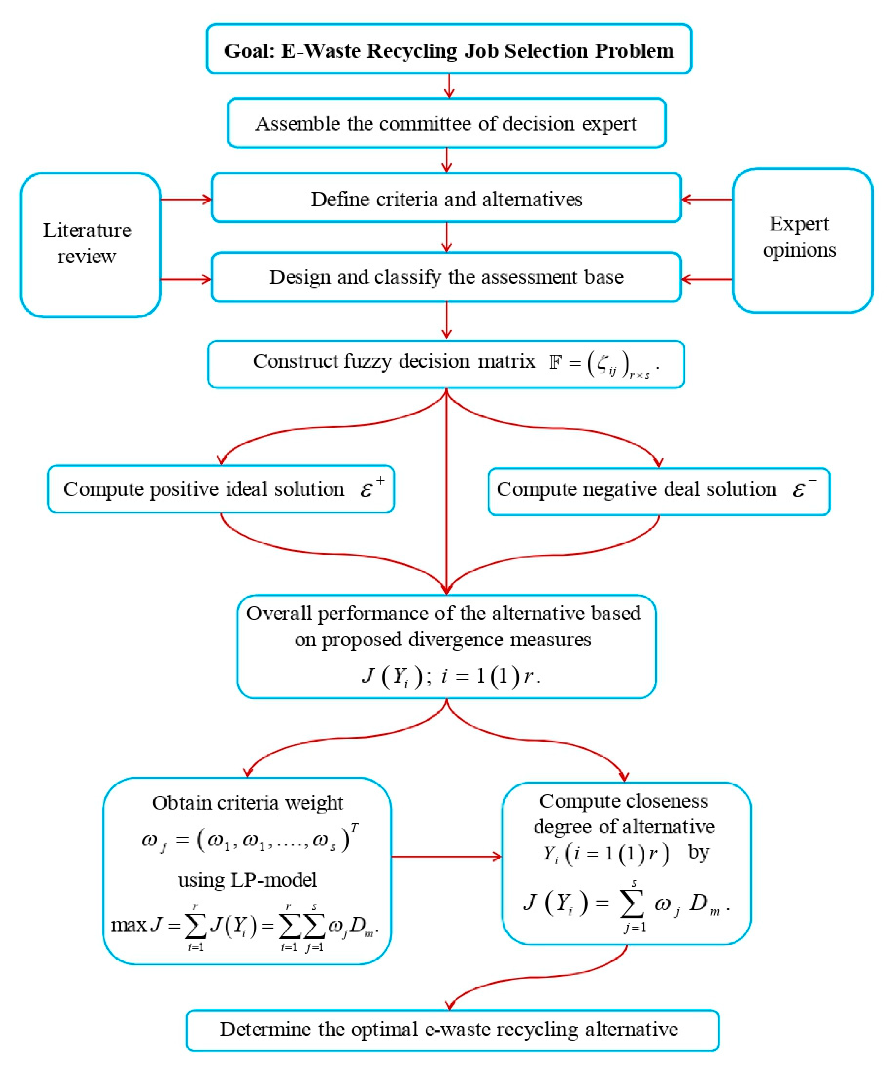
The evolution of the fuzzy MCDM method is according to the conception of the degree of optimality rooted in an option where multiple criteria distinguish the concept of the desirable option. This perception has been applied extensively by the MCDM approach known technique for order preference by similarity to the ideal solution. As considered by the notion, the most desirable option should not only have the shortest distance from the ideal option but also have the longest distance from the anti-ideal option.
Based on the concept, the overall preference value of an option is computed by its divergences to the ideal solution and the anti-ideal solution. This divergence is thus interrelated with the criteria weights and should be incorporated in the divergence measure. To handle the issue, the fuzzy MCDM method developed uses the optimal criteria weights and the optimal dimension weights, as shown in Figure 1 and discussed in Section 4, to weight the divergence between the option and the ideal/anti-ideal option. The proposed method was implemented to evaluate the recycling job selection problem of sustainable planning of the e-waste as follows:
Definition 3.
A triangular fuzzy number (TFN) ζ is given by triplet ( f , g , h ) . The membership function μ ζ ( x ) is defined as follows:
μ ζ ( x ) = { 0 , x f x f g f , f x g x h g h , g x h 0 , x h .
The linguistic variable refers to those expressed in form of linguistic ratings. The philosophy of linguistic variables is highly constructive in handling with circumstances of a high complexity level or imprecision to be logically expressed in the form of traditional quantitative phenomenon. Such linguistic values are characterized by fuzzy numbers (FNs). Table 1 demonstrates linguistic values for weights and ratings.
Now, to develop a fuzzy MCDM approach, the canonical demonstration of operation on TFN is implemented, which is associated with the graded mean integration representation model [41].
Definition 4
(Chou [41]). For TFN ζ i j = ( f i j , g i j , h i j ) the graded mean integration representation of TFN ζ i j is defined by
P ( ζ i j ) = f i j + 4 g i j + h i j 6 .
Next, linear normalization is applied to the transformation of different criteria scale into a similar scale since it has simple calculations instead of vector normalization. As a result, here is constructed the normalized triangular fuzzy matrix represented by Ζ = ( ζ i j ) m × n , where
ζ = ( f i j h j , g i j h j , h i j h j ) , j v b ;
and
ζ = ( f j f i j , f j g i j , f j h i j ) , j v n ;
such that
h j = max i h i j i f j v b   and   f j = min i f i j i f j v n .
where v b and v n stand for the set of criteria in terms of beneficial and non-beneficial, respectively.
Generally, an MCDM problem can be sketchily demonstrated as
Z 1 Z 2 Z s F = Y 1 Y 2 Y r [ ξ 11 ξ 11 ξ 1 ξ 21 ξ 22 ξ 2 s ξ r 1 ξ r 2 ξ r s ]
where Y = { Y 1 , Y 2 , , Y r } and Z = { Z 1 , Z 2 , , Z s } are the sets of alternatives and criteria, respectively, and ζ i j = ( f i j , g i j , h i j ) ; i = 1 ( 1 ) r , j = 1 ( 1 ) s present the fuzzy numbers.
Let the MCDM problems consist of r alternatives Y i ( i = 1 ( 1 ) r ) such that alternative is achieved by means of S criteria Z j ( j = 1 ( 1 ) s ) . ζ i j is constructed by alternative Y i ( i = 1 ( 1 ) r ) with respect to criterion Z j ( j = 1 ( 1 ) s ) , are fuzzy values (FVs). Let ω j be the weight of criterion with the condition that ω j 0 , j = 1 s ω j = 1 . Here, ω j = ( ω 1 , ω 2 , , ω s ) T symbolizes the set of known information, this is generated by decision experts in the form of linear constraints, concerning the criterion weights. It is worth mentioning that the proposed method is appropriate for circumstances where the number of decision experts is small such that they assess the criterion based on their experience and knowledge and the alternatives could be of any type, then assessment of alternatives is constructed in the form of FVs.
The developed approach is implemented to solve the MCDM problems with partially or completely unknown criteria’s weights information. This method consists of the subsequent steps (see Figure 1):
Step 1:
Construct the fuzzy decision matrix F = ( ζ i j ) r × s .
The decision experts furnish all the feasible assessments regarding the alternative Y i concerning criterion Z j , mentioned by fuzzy numbers (FNs) ζ i j = ( f i j , g i j , h i j ) ; i = 1 ( 1 ) r , j = 1 ( 1 ) s which are obtained based on Table 1 and Equations (43) and (44) and demonstrated in Equation (48).
Step 2:
Compute ideal solution (IS) and anti-ideal solution (A-IS).
The optimal values (or IS) for diverse criterion are altered and pointed out as
ε + = { max i = 1 ( 1 ) r ζ i j for benefit criterion v j min i = 1 ( 1 ) s ζ i j for cos t criterion v j ,   for   j = 1 ( 1 ) s .
Similarly, the worst values (or A-IS) for diverse criterion is given by
ε = { min i = 1 ( 1 ) r ζ i j for benefit criterion v j max i = 1 ( 1 ) s ζ i j for cos t criterion v j   for   j = 1 ( 1 ) s .
Step 3:
Compute the criteria weights
In case the information about the criterion weight ω j is partially known, then the criterion weights can be evaluated in advance. Based on the divergence measure analysis, we developed a nonlinear programming model for the purpose of selecting the criterion weight vector ω j ; it will maximize all of the deviation values for the alternatives.
According to (14), we evaluated D m i j + ( ζ i j , ε + ) and D m i j ( ζ i j , ε ) as follows:
D m i j + ( ζ i j , ε + ) = i = 1 n [ ( μ ζ i j ( x i ) + μ ε + ( x i ) ) ( μ ζ i j ( x i ) μ ε + ( x i ) ) 2 μ ζ i j ( x i ) μ ε + ( x i ) ln ( ( μ ζ i j ( x i ) + μ ε + ( x i ) ) 2 μ ζ i j ( x i ) μ ε + ( x i ) ) + ( 2 μ ζ i j ( x i ) μ ε + ( x i ) ) ( μ ε + ( x i ) μ ζ i j ( x i ) ) 2 ( 1 μ ζ i j ( x i ) ) ( 1 μ ε + ( x i ) ) ln ( ( 2 μ ζ i j ( x i ) μ ε + ( x i ) ) 2 ( 1 μ ζ i j ( x i ) ) ( 1 μ ε + ( x i ) ) ) ] ,
D m i j ( ζ i j , ε ) = i = 1 n [ ( μ ζ i j ( x i ) + μ ε ( x i ) ) ( μ ζ i j ( x i ) μ ε ( x i ) ) 2 μ ζ i j ( x i ) μ ε ( x i ) ln ( ( μ ζ i j ( x i ) + μ ε ( x i ) ) 2 μ ζ i j ( x i ) μ ε ( x i ) ) + ( 2 μ ζ i j ( x i ) μ ε ( x i ) ) ( μ ε ( x i ) μ ζ i j ( x i ) ) 2 ( 1 μ ζ i j ( x i ) ) ( 1 μ ε ( x i ) ) ln ( ( 2 μ ζ i j ( x i ) μ ε ( x i ) ) 2 ( 1 μ ζ i j ( x i ) ) ( 1 μ ε ( x i ) ) ) ] .
Next, the overall performance of the alternative u i computed by the given formula
J ( Y i ) = j = 1 n ω j D m i j ,
where
D m i j = D m i j D m i j + D m i j + .
Apparently, the larger value of J ( Y i ) shows the superior option. Thus, all the alternatives are measured as a whole to construct a combined weight vector. Thus, LP-model is demonstrated as below:
max J = i = 1 m J ( Y i ) = i = 1 m j = 1 n ω j D m i j s .   t .   { ω W , ω j 0 , j = 1 s ω j = 1 , j = 1 ( 1 ) s .
Step 4:
Compute the closeness degree of the alternative(s).
Based on (53), the closeness degree J ( Y i ) of each alternative Y i ( i = 1 ( 1 ) r ) regarding the ideal solution is evaluated.
Step 5:
Rank the alternatives.
Choose the biggest value, which is signified by J ( Y k ) , among the values J ( Y i ) , i = 1 ( 1 ) r . Thus, Y k is the best option.

5. Investigating the Sustainable Planning of an E-Waste Recycling Job Selection

In the global climate change and global warming, the three entities of society, economy, and environment are in an inseparable connection with each other [42,43]. Such interconnection has caused human well-being to be closely dependent on the environment health condition [44,45]. In consequence, we can see the aftermaths of such conditions in the form of complicated challenges that have already occurred as sustainability challenges [46]. Clearly, the natural resources are being exhausted, but simultaneously the demand of society is increasingly rising, which has placed a disparaging pressure upon the environment, economy, and society [33]. One of the typical instances of sustainability challenges is an electronic waste (e-waste) [47]; this is a problem of high complexity in its nature, it does not seem to be solvable at all, and this is of a socio-ecological scale. E-waste emerges with discarding the electronic products like cellular phones, computers, and other electronic appliances we are using daily. As can be easily understood, the last few decades have witnessed a vast evolution of the electrical and electronics industry [48]. There has been an extraordinary rise in consuming electronic equipment, especially computers and mobile phones. This tremendous increase in consumption has led to the accumulation of waste electrical and electrical equipment (WEEE) [49,50,51], which is normally discussed under the title of E-waste [52]. Across the globe, electronic equipment usage has become an indispensable part of daily life. Currently, there is a big pressure from academic communities, interest groups, environmental watchdogs, etc. on electronic producers and local industries to bring into action the effective management mechanisms in a way to make efficient response to the perceived and potential e-waste problems.
To deal with the e-waste recycling planning issues pointed above, we proposed a novel sustainable planning method for meeting the best sustainability interests of an e-recycling company. The method utilizes a fuzzy MCDM approach and a series of optimal weighting approaches to find and choose the option recycling activities for e-waste recycling jobs of an e-recycling company. It shows an innovative contribution to the procedural development of weighting the three dimensions of corporate sustainability for planning decisions.
In this section, a case study of recycling partner selection in sustainable planning of e-waste was presented, aiming at showing the viability of the proposed approach. The proposed method was utilized to rank the given recycling associations in India. Let Y 1 , Y 2 , Y 3 , and Y 4 are four selected associations that conduct the recycling procedures for products that are end-of-life vehicles, scraped electronics, scraped metals, scraped paper recycling, as well as dismasting operations. These four associations were computed based on given inter-independent criterion set { Z 1 , Z 2 , Z 3 , Z 4 , Z 5 } . Out of these first, second and fourth were benefit criteria, while third and fifth were cost criteria. In order to choose an appropriate sustainable recycling partner, the proposed approach was applied and evaluated as follows: after preliminary screening, four potential alternatives of this company were considered, which are denoted as Y i (i = 1, 2, ..., 4) with most favorable performance assessment of the e-waste options on qualitative sustainability criteria (given in Table 2). An expert group consisting of three decision-makers (D1, D2, D3, and D4) was established for the purpose of doing the performance rating of each e-waste option. The decision-makers’ weights were assumed as ϖ 1 = 0.25 , ϖ 2 = 0.25 , ϖ 3 = 0.25 , ϖ 4 = 0.25 , since they had different levels of technical knowledge and expertise. The next step was to estimate the best e-waste recycling partner selection through the proposed method. To estimate the best e-waste recycling partner option, the decision experts (DEs) assumption was that each criterion is beneficial. Table 3 depicts the estimation values in terms of linguistic values constructed by e-waste recycling partner decision experts.
Here, evaluating the mean values of fuzzy scores of the estimation outcomes allocated by DEs, we achieved the estimation matrix. Afterward, Equations (45)–(47) were implemented to construct a triangular fuzzy normalized estimation matrix (see Table 4). Later on, the ratings were transformed into crisp values on the basis of Definition 4. After that, the normalized F-DM was created according to Equation (44), is presented in Table 5.
Here, there is a group of experts to make decisions on choosing the recycling partner. The decision experts furnish all the feasible evaluations regarding the alternative Y i with respect to criterion Z j , and construct aggregated decision matrix, which is given in Table 5 associated with Table 1 and Equations (43) and (47). According to their knowledge and experience regarding the criterion set, partial information of the weights is given by
W = { ( ω j ) T | 0.2 ω 1 0.35 , 0.1 ω 2 0.27 , 0.15 ω 3 0.25 , ω 1 0.2 ω 4 , 0.08 ω 4 0.15 , 0.2 ω 5 0.4 , ω 2 ω 5 ω 3 } such   that   j = 1 s ω j = 1 .
Step 1:
Fuzzy IS and A-IS are calculated by using (49) and (50) are as follows:
ε + = { 0.757 , 0.76 , 0.231 , 0.317 , 0.244 } ,
ε = { 0.24 , 0.25 , 0.767 , 0.229 , 0.77 } .
Step 2:
Corresponding to (51) and (52), the divergence measure of ζ i j form ε + and ζ i j form ε are evaluated as follows:
D m 11 + = 0.3021 , D m 12 + = 0.0000 , D m 13 + = 0.0000 , D m 14 + = 0.0236 , D m 15 + = 0.0000 , D m 21 + = 0.2211 , D m 22 + = 0.3913 , D m 23 + = 0.5253 , D m 24 + = 0.0000 , D m 25 + = 0.4674 , D m 31 + = 0.0000 , D m 32 + = 0.0000 , D m 33 + = 0.000566 , D m 34 + = 0.1138 , D m 35 + = 0.0000315 , D m 41 + = 0.4910 , D m 42 + = 0.058 , D m 43 + = 0.0089 , D m 44 + = 0.0015 , D m 45 + = 0.0053 .
And
D m 11 = 0.0000525 , D m 12 = 0.3913 , D m 13 = 0.5253 , D m 14 = 0.008647 , D m 15 = 0.4674 , D m 21 = 0.0004378 , D m 22 = 0.0000 , D m 23 = 0.0000 , D m 24 = 0.1138 , D m 25 = 0.0000 , D m 31 = 0.4583 , D m 32 = 0.3913 , D m 33 = 0.2478 , D m 34 = 0.0000 , D m 35 = 0.3250 , D m 41 = 0.0000 , D m 42 = 0.0101 , D m 43 = 0.1009 , D m 44 = 0.0172 , D m 45 = 0.1081 .
Next, the overall performances, by using (53), of alternative are calculated as follows:
D m 11 = 0.0001737 , D m 12 = 1.0000 , D m 13 = 1.0000 , D m 14 = 0.2681 , D m 15 = 1.0000 , D m 21 = 0.0020 , D m 22 = 0.0000 , D m 23 = 0.0000 , D m 24 = 1.0000 , D m 25 = 0.0000 , D m 31 = 1.0000 , D m 32 = 1.0000 , D m 33 = 0.9977 , D m 34 = 0.0000 , D m 35 = 0.9999 , D m 41 = 0.0000 , D m 42 = 0.1483 , D m 43 = 0.9189 , D m 44 = 0.9198 , D m 45 = 0.9533 .
Step 3:
To compute the weight vector, construct the model
max J = 1.0022 ω 1 + 2.1483 ω 2 + 2.9166 ω 3 + 2.1879 ω 4 + 2.9532 ω 5 s . t . { 0.25 ω 1 0.4 , 0.16 ω 2 0.27 , 0.1 ω 4 0.18 , 0.2 ω 5 0.35 , 0.15 ω 3 0.25 , ω 1 0.2 ω 4 , ω 5 ω 2 ω 3 ω j = ( ω 1 , ω 2 , , ω s ) T , ω j 0 , j = 1 s ω j = 1 .
Using MATHEMATICA, model (57) is computed and the criteria’s weight vector is computed by
( ω j ) T = ( 0.25 , 0.16 , 0.165 , 0.1 , 0.325 ) T .
Step 4:
The calculated closeness degrees of the alternatives are given as
J ( Y 1 ) = 0.6769 , J ( Y 2 ) = 0.1005 , J ( Y 3 ) = 0.8996 , J ( Y 4 ) = 0.5771 .
Step 5:
Based on calculated closeness degrees of the alternatives, the ranking of the associations is Y 3 Y 1 Y 4 Y 2 .
Hence, a suitable e-waste recycling job is Y 3 .

Comparison and Discussion for the Sustainable Planning of an E-Waste Recycling Job Selection

The grading of given associations is also acquired by the TOPSIS, F-TOPSIS, intuitionistic fuzzy TOPSIS, and proposed methods, and is presented in Table 6.
We observed that there was no discrepancy in the grading order of the e-waste recycling job options by the TOPSIS method, F-TOPSIS method, IF-TOPSIS methods, and proposed method. Hence, all the methods provided the unique optimal alternative Y3, i.e., desirable e-waste recycling job. In general, the advantages of the extended approach over the existing methods are presented by
  • The portrayal of the relative significance of various criteria is made simple with the help of linguistic evaluations enabling the attainment of the desirable stability between parameter performance and desirable e-waste recycling job in various circumstances.
  • The aggregation of various criteria (e.g., health and safety at workplace, public acceptability, and green technology innovation) is performed efficiently with the proposed method whereas, the preference order abnormality problem is evaded with the help of objective utility functions.
  • The developed method utilizes a conventional concept of the synchronized satisfaction of the given objectives that comprises the compromise doctrine of TOPSIS, that is, to be as closer as likely to an IS and as farther as likely from an A-IS.
  • The aggregation of various criteria is made with FSR TOPSIS Chamodrakas, et al. [57], a proposed method to evade possible inconsistency of the ranking outcomes. Furthermore, the utilization of parameterized utility functions for evaluating the normalized decision matrix in FSR TOPSIS reduces the order abnormality concern.
  • As the significance of DEs is considered, we have discussed a method based graded mean integration representation (GMIR) of TFN, which provides more precise outcomes for MCDM problems.
From the analyses presented above, the proposed method based on divergence measures of FSs has the following advantages.
First, FSs used in this paper can express the evaluation information more flexibly. They can embed several values in membership degrees and can retain the completeness of original data or the inherent thoughts of decision-makers, which is the prerequisite of guaranteeing the accuracy of final outcomes.
Second, the proposed fuzzy divergence measures are different from the existing divergence measures that always involve the extensions whose impact on the final solution may be considerable, because the proposed divergence measures can include the advantages of parametric generalization, and overcome these shortcomings. This can avoid losing and distorting the preference information provided, which makes the final results better correspond with real decision-making problems.
Finally, the proposed method can provide a useful and flexible way to efficiently facilitate the decision-making process within the fuzzy environment. Moreover, the first method could handle some special cases where the weight information is not always available and instead only partial knowledge of criteria weights may be obtained as a group of linear constraints.

6. Conclusions

In the present study, we introduced some new divergence measures for FSs, which are generalizations of probabilistic divergence measures and discussed some elegant properties, which shows the strength of the proposed measures. Later on, we defined a family of unified divergence measures for FSs based on various types of entropy function. Next, an approach, which is based on the fuzzy divergence measure to determine the weights of criteria, was developed for MCDM problems within the fuzzy atmosphere. The criteria with large cross-entropy and small entropy need to be well taken into account. Finally, we implemented the proposed method with an example that demonstrated its applicability and effectiveness in comparison to the results of the methods already proposed in the literature.
The advantages of the proposed method were that they could be easily and conveniently evaluated and they could efficiently reduce the loss of information estimation. The method proposed in this study was proved both feasible and valid through the example illustration of recycling partner selection of sustainable practices and comparison with existing methods. Thus, proposed method had vast application potential for solving MCDM problems in FSs, where alternatives were constructed with regard to the criterion set in terms of FVs, and the criterion weights were partially known. In the future, we would enlarge our research to IF-divergence measures and interval-valued intuitionistic fuzzy-divergence measures and implement various real-life applications.

Author Contributions

Conceptualization, P.R. and Y.Y.; methodology, P.R.; software, A.R.M. validation, A.M., M.A. and A.M.; formal analysis, A.R.M.; resources, A.M.; writing—original draft preparation, M.A.; writing—review and editing, D.S.H. supervision, K.G.; project administration, K.G. All authors have read and agreed to the published version of the manuscript.

Funding

This research was supported by Ton Duc Thang University.

Conflicts of Interest

The authors declare no conflict of interest.

References

  1. Zadeh, L.A. Fuzzy sets. Inf. Control 1965, 8, 338–353. [Google Scholar] [CrossRef] [Green Version]
  2. Zadeh, L.A. Fuzzy algorithms. Inf. Control 1968, 12, 94–102. [Google Scholar] [CrossRef] [Green Version]
  3. De Luca, A.; Termini, S. A definition of a nonprobabilistic entropy in the setting of fuzzy sets theory. Inf. Control 1972, 20, 301–312. [Google Scholar] [CrossRef] [Green Version]
  4. Pal, N.R.; Pal, S.K. Object-background segmentation using new definitions of entropy. IEE Proc. E Comput. Digit. Tech. 1989, 136, 284–295. [Google Scholar] [CrossRef] [Green Version]
  5. Bhandari, D.; Pal, N.R. Some new information measures for fuzzy sets. Inf. Sci. 1993, 67, 209–228. [Google Scholar] [CrossRef]
  6. Kullback, S.; Leibler, R.A. On information and sufficiency. Ann. Math. Stat. 1951, 22, 79–86. [Google Scholar] [CrossRef]
  7. Shang, X.G.; Jiang, W.S. A note on fuzzy information measures. Pattern Recognit. Lett. 1997, 18, 425–432. [Google Scholar] [CrossRef]
  8. Lin, J.H. Divergence measure based on shannon entropy. IEEE Trans. Inf. Theory 1991, 37, 145–151. [Google Scholar] [CrossRef] [Green Version]
  9. Montes, S.; Couso, I.; Gil, P.; Bertoluzza, C. Divergence measure between fuzzy sets. Int. J. Approx. Reason. 2002, 30, 91–105. [Google Scholar] [CrossRef] [Green Version]
  10. Kumar, P.; Chhina, S. A symmetric information divergence measure of the csiszar’s f-divergence class and its bounds. Comput. Math. Appl. 2005, 49, 575–588. [Google Scholar] [CrossRef] [Green Version]
  11. Fisher, R.A. Theory of statistical estimation. Math. Proc. Camb. Philos. Soc. 1925, 22, 700–725. [Google Scholar] [CrossRef] [Green Version]
  12. Fan, J.L.; Xie, W.X. Distance measure and induced fuzzy entropy. Fuzzy Sets Syst. 1999, 104, 305–314. [Google Scholar] [CrossRef]
  13. Wang, Z.; Guo, D.; Wang, X.; Zhang, B.; Wang, B. How does information publicity influence residents’ behaviour intentions around e-waste recycling? Resour. Conserv. Recycl. 2018, 133, 1–9. [Google Scholar] [CrossRef]
  14. Mishra, A.R.; Rani, P. Shapley divergence measures with vikor method for multi-attribute decision-making problems. Neural Comput. Appl. 2019, 31, 1299–1316. [Google Scholar] [CrossRef]
  15. Hwang, C.L.; Yoon, K. Multiple Attribute Decision Making: Methods and Applications; Springer: New York, NY, USA, 1981. [Google Scholar]
  16. Zeleny, M. Multiple Criteria Decision Making Kyoto 1975; Springer Science & Business Media: Berlin, Germany, 2012; Volume 123. [Google Scholar]
  17. Belton, V.; Stewart, T.; Hobbs, B.F. Multiple Criteria Decision Analysis: An Integrated Approach; Springer Science & Business Media: Berlin, Germany, 2002. [Google Scholar]
  18. De Brucker, K.; Macharis, C.; Verbeke, A. Multi-criteria analysis and the resolution of sustainable development dilemmas: A stakeholder management approach. Eur. J. Oper. Res. 2013, 224, 122–131. [Google Scholar] [CrossRef]
  19. Insua, D.R. Sensitivity analysis in multi-objective decision making. In Sensitivity Analysis in Multi-Objective Decision Making; Springer: Berlin, Germany, 1990; pp. 74–126. [Google Scholar]
  20. Valentinaa, F.; Ireneb, P.; Alexisb, T. Supporting decisions in public policy making processes: Generation of alternatives and innovation. Eur. J. Oper. Res. 2017. [Google Scholar]
  21. Pareto, V. Cours d’économie politique. Trav. Sci. Soc. 1964, 1–424. [Google Scholar]
  22. Yu, P.-L. A class of solutions for group decision problems. Manag. Sci. 1973, 19, 936–946. [Google Scholar] [CrossRef]
  23. Awasthi, A.K.; Cucchiella, F.; D’Adamo, I.; Li, J.; Rosa, P.; Terzi, S.; Wei, G.; Zeng, X. Modelling the correlations of e-waste quantity with economic increase. Sci. Total. Environ. 2018, 613, 46–53. [Google Scholar] [CrossRef]
  24. Ilankoon, I.M.S.K.; Ghorbani, Y.; Chong, M.N.; Herath, G.; Moyo, T.; Petersen, J. E-waste in the international context—A review of trade flows, regulations, hazards, waste management strategies and technologies for value recovery. Waste Manag. 2018, 82, 258–275. [Google Scholar] [CrossRef]
  25. Li, K.; Xu, Z. A review of current progress of supercritical fluid technologies for e-waste treatment. J. Clean. Prod. 2019, 227, 794–809. [Google Scholar] [CrossRef]
  26. Otto, S.; Kibbe, A.; Henn, L.; Hentschke, L.; Kaiser, F.G. The economy of e-waste collection at the individual level: A practice oriented approach of categorizing determinants of e-waste collection into behavioral costs and motivation. J. Clean. Prod. 2018, 204, 33–40. [Google Scholar] [CrossRef]
  27. Sajid, M.; Syed, J.H.; Iqbal, M.; Abbas, Z.; Hussain, I.; Baig, M.A. Assessing the generation, recycling and disposal practices of electronic/electrical-waste (e-waste) from major cities in pakistan. Waste Manag. 2019, 84, 394–401. [Google Scholar] [CrossRef] [PubMed]
  28. Zhang, B.; Du, Z.; Wang, B.; Wang, Z. Motivation and challenges for e-commerce in e-waste recycling under “big data” context: A perspective from household willingness in china. Technol. Forecast. Soc. Chang. 2019, 144, 436–444. [Google Scholar] [CrossRef]
  29. Yeh, C.-H.; Xu, Y. Sustainable planning of e-waste recycling activities using fuzzy multicriteria decision making. J. Clean. Prod. 2013, 52, 194–204. [Google Scholar] [CrossRef]
  30. Xu, Y.; Yeh, C.-H. Sustainability-based selection decisions for e-waste recycling operations. Ann. Oper. Res. 2017, 248, 531–552. [Google Scholar] [CrossRef]
  31. Shannon, C.E. A mathematical theory of communication. Bell Syst. Tech. J. 1948, 27, 379–423. [Google Scholar] [CrossRef] [Green Version]
  32. Rényi, A. On measures of entropy and information. In Proceedings of the Fourth Berkeley Symposium on Mathematical Statistics and Probability, Berkeley, CA, USA, 20 June–30 July 1960; The Regents of the University of California: Berkeley, CA, USA, 1961. [Google Scholar]
  33. Ghisellini, P.; Cialani, C.; Ulgiati, S. A review on circular economy: The expected transition to a balanced interplay of environmental and economic systems. J. Clean. Prod. 2016, 114, 11–32. [Google Scholar] [CrossRef]
  34. Kullback, S. Information Theory and Statistics; Courier Corporation: North Chelmsford, MA, USA, 1968. [Google Scholar]
  35. Bajaj, R.K.; Hooda, D. On some new generalized measures of fuzzy information. World Acad. Sci. Eng. Technol. 2010, 62, 747–753. [Google Scholar]
  36. Taneja, I.J.; Pardo, L.; Morales, D.; Menéndez, M.L. On generalized information and divergence measures and their applications: A brief review. Qüestiió Quaderns D’estadística i Investigació Operativa 1989, 13, 47–73. [Google Scholar]
  37. Le Cam, L. Asymptotic Methods in Statistical Decision Theory; Springer Science & Business Media: Berlin, Germany, 1986. [Google Scholar]
  38. Parkash, O. Mukesh, two new symmetric divergence measures and information inequalities. Int. J. Math. Appl. 2011, 4, 165–179. [Google Scholar]
  39. Sibson, R. Information radius. Zeitschrift für Wahrscheinlichkeitstheorie und verwandte Gebiete 1969, 14, 149–160. [Google Scholar] [CrossRef]
  40. Sharma, B.; Mittal, D. New non-additive measures of relative information. J. Comb. Inf. Syst. Sci. 1977, 2, 122–132. [Google Scholar]
  41. Chou, C.C. The canonical representation of multiplication operation on triangular fuzzy numbers. Comput. Math. Appl. 2003, 45, 1601–1610. [Google Scholar] [CrossRef] [Green Version]
  42. Bringezu, S.; Bleischwitz, R. Sustainable Resource Management: Global Trends, Visions and Policies; Routledge: Abingdon, UK, 2017. [Google Scholar]
  43. Meadowcroft, J.; Steurer, R. Assessment practices in the policy and politics cycles: A contribution to reflexive governance for sustainable development? J. Environ. Policy Plan. 2018, 20, 734–751. [Google Scholar] [CrossRef]
  44. Clarke-Sather, A.; Cobb, K. Onshoring fashion: Worker sustainability impacts of global and local apparel production. J. Environ. Policy Plan. 2019, 208, 1206–1218. [Google Scholar] [CrossRef]
  45. Breen, S.-P.W.; Loring, P.A.; Baulch, H. When a water problem is more than a water problem: Fragmentation, framing, and the case of agricultural wetland drainage. Front. Environ. Sci. 2018, 6, 129. [Google Scholar] [CrossRef]
  46. Jerome, L. What do citizens need to know? An analysis of knowledge in citizenship curricula in the uk and ireland. Comp. A J. Comp. Int. Educ. 2018, 48, 483–499. [Google Scholar] [CrossRef]
  47. Cruz-Sotelo, S.; Ojeda-Benítez, S.; Jáuregui Sesma, J.; Velázquez-Victorica, K.; Santillán-Soto, N.; García-Cueto, O.; Alcántara Concepción, V.; Alcántara, C. E-waste supply chain in mexico: Challenges and opportunities for sustainable management. Sustainability 2017, 9, 503. [Google Scholar] [CrossRef] [Green Version]
  48. Zidan, M.A.; Strachan, J.P.; Lu, W.D. The future of electronics based on memristive systems. Nat. Electron. 2018, 1, 22–29. [Google Scholar] [CrossRef]
  49. Casey, K.; Lichrou, M.; Fitzpatrick, C. Treasured trash? A consumer perspective on small waste electrical and electronic equipment (weee) divestment in ireland. Resour. Conserv. Recycl. 2019, 145, 179–189. [Google Scholar] [CrossRef]
  50. Stubbings, W.A.; Nguyen, L.V.; Romanak, K.; Jantunen, L.; Melymuk, L.; Arrandale, V.; Diamond, M.L.; Venier, M. Flame retardants and plasticizers in a canadian waste electrical and electronic equipment (weee) dismantling facility. Sci. Total Environ. 2019, 675, 594–603. [Google Scholar] [CrossRef] [PubMed]
  51. Diani, M.; Pievatolo, A.; Colledani, M.; Lanzarone, E. A comminution model with homogeneity and multiplication assumptions for the waste electrical and electronic equipment recycling industry. J. Clean. Prod. 2019, 211, 665–678. [Google Scholar] [CrossRef]
  52. Gu, W.; Bai, J.; Feng, Y.; Zhang, C.; Wang, J.; Yuan, W.; Shih, K. Chapter 9—biotechnological initiatives in e-waste management: Recycling and business opportunities. In Electronic Waste Management and Treatment Technology; Prasad, M.N.V., Vithanage, M., Eds.; Butterworth-Heinemann: Oxford, UK, 2019; pp. 201–223. [Google Scholar]
  53. Tzeng, G.-H.; Huang, J.-J. Multiple Attribute Decision Making: Methods and Applications; Chapman and Hall/CRC: London, UK, 1981. [Google Scholar]
  54. Chen, C.-T. Extensions of the topsis for group decision-making under fuzzy environment. Fuzzy Sets Syst. 2000, 114, 1–9. [Google Scholar] [CrossRef]
  55. Joshi, D.; Kumar, S. Intuitionistic fuzzy entropy and distance measure based topsis method for multi-criteria decision making. Egypt. Inform. J. 2014, 15, 97–104. [Google Scholar] [CrossRef]
  56. Mishra, A.R.; Rani, P.; Jain, D. Information measures based topsis method for multicriteria decision making problem in intuitionistic fuzzy environment. Iran. J. Fuzzy Syst. 2017, 14, 41–63. [Google Scholar]
  57. Chamodrakas, I.; Alexopoulou, N.; Martakos, D. Customer evaluation for order acceptance using a novel class of fuzzy methods based on topsis. Expert Syst. Appl. 2009, 36, 7409–7415. [Google Scholar] [CrossRef]
Figure 1. Procedure of the proposed method for multi-criteria decision-making (MCDM) problems.
Symmetry 12 00090 g001
Table 1. Linguistic values for evaluating sustainability assessment of e-waste products.
Linguistic TermsFuzzy Score
Very Strong (VS)(0.7, 0.9, 1.0)
Fairly Strong (FS)(0.5, 0.7, 0.9)
Equal (E)(0.3, 0.5, 0.7)
Fairly Weak (FW)(0.1, 0.3, 0.5)
Very Weak (VW)(0.0, 0.1, 0.3)
Table 2. The overall explanation of e-waste recycling job selection problem.
Sustainability Criteria under Each DimensionFirm’s E-Waste ProductsAlternatives of the E-Waste Recycling Job
Sustainability DimensionSustainability CriteriaDescriptionE-Waste ProductDescription
Social ( S ) Health and safety
at the workplace ( Z 1 )
The number of decreased
workers’ compensation
claimed
ComputerPersonal computers, CRT monitors, notebook computers, PC keyboards,
LCD monitors, modem, cables associated
with PC system, mouse, etc.
Y 1
Public acceptability ( Z 2 ) General attitudes/
public perceptions regard to the firms’ e-recycling
services
Communication
equipment
Server, telephone handsets,
hub, rack mount cabinets, routers, switch, assorted network gear, PABX controller units,
modems/print servers, uninterruptible power supplies, etc.
Economic ( E c ) Direct/Indirect cost ( Z 3 ) The expenditure is given/The expenses for exploring business opportunitiesBatteryLead acid batteries, lithium ion, lithium batteries,
NiCad batteries (vented/sealed), NiMH batteries,
Alkaline batteries, etc.
Y 2
Environmental ( E n ) Green technology Innovation ( Z 4 ) The new technology innovations Made to decrease the negative environmental EffectsCell phoneCell phones, battery, charger,
accessories, etc.
Y 3
The problem decreased the volume of trash/waste within the landfillOffice electrical equipmentDesktop printers, enterprise printer, photocopy machines,
fax machines, desktop scanners, desktop
multifunction printers/scanners, etc.
Landfill reduction ( Z 5 ) Consumer electrical equipmentCRT televisions, LCD televisions, plasma televisions,
VCR/DVD/set top box, speaker devices, Hi-Fi stereo,
domestic vacuum cleaners, microwave ovens,
cordless phones, digital still cameras, video cameras, etc.
Y 4
Table 3. Evaluation of e-waste recycling job alternatives in linguistic values.
Z 1 Z 2 Z 3 Z 4 Z 5
Y 1 (E,VW,FW,VW)(VS,E,VS,VS)(FW,FW,VW,VW)(FW,VW,FW,VW)(FW,FW,E,VW)
Y 2 (FW,FW,E,VW)(FW,FW,FW,VW)(VS,VS,VS,E)(VW,VW,VW,VW)(VS,VS,FS,FS)
Y 3 (FS,VS,FS,FS)(VS,FS,FS,FS)(FS,FW,VW,VW)(FS,VW,FW,VW)(VW,VW,FW,E)
Y 4 (E,FW,FW,VW)(FS,E,FW,FW)(FS,FW,E,VW)(VW,VW,VW,FW)(VS,FW,FW,VW)
Table 4. Triangular fuzzy evaluation matrix for e-waste recycling job selection problem.
Z 1 Z 2 Z 3 Z 4 Z 5
Y 1 (0.1,0.25,0.45)(0.6,0.8,0.93)(0.05,0.2,0.4)(0.05,0.2,0.35)(0.13,0.3,0.5)
Y 2 (0.15,0.35,0.5)(0.08,0.25,0.45)(0.6,0.8,0.93)(0.0,0.1,0.3)(0.65,0.8,0.95)
Y 3 (0.55,0.75,0.93)(0.5,0.75,0.9)(0.15,0.3,0.5)(0.1,0.3,0.5)(0.1,0.2,0.45)
Y 4 (0.12,0.3,0.5)(0.25,0.45,0.65)(0.23,0.4,0.6)(0.03,0.15,0.35)(0.22,0.4,0.55)
Table 5. Aggregated fuzzy decision matrix for e-waste recycling job selection problem.
Z 1 Z 2 Z 3 Z 4 Z 5
Y 1 0.28440.760.2310.2290.244
Y 2 0.3150.250.7670.0950.77
Y 3 0.7570.7510.3190.3170.275
Y 4 0.240.4350.4110.1570.391
Table 6. Comparison of grading order of alternatives from various methods.
MethodsBenchmarkRankingOptimal Alternative
TOPSIS Tzeng and Huang [53] methodCrisp Sets Y 3 Y 4 Y 1 Y 2 Y 3
F-TOPSIS Chen [54] methodFuzzy sets and distance measure Y 3 Y 1 Y 4 Y 2 Y 3
IF-TOPSIS Joshi and Kumar [55] methodIntuitionistic fuzzy sets and distance measure Y 3 Y 1 Y 4 Y 2 Y 3
IF-TOPSIS Mishra, et al. [56] method Intuitionistic fuzzy sets and similarity measure Y 3 Y 1 Y 4 Y 2 Y 3
Proposed method Fuzzy sets and divergence measure based linear programming model Y 3 Y 1 Y 4 Y 2 Y 3

