Eliciting Correlated Weights for Multi-Criteria Group Decision Making with Generalized Canonical Correlation Analysis


Graduate Program in Applied Informatics, University of Fortaleza, Fortaleza 60811-905, CE, Brazil
*
Authors to whom correspondence should be addressed.
Symmetry 2020, 12(10), 1612; https://0-doi-org.brum.beds.ac.uk/10.3390/sym12101612
Submission received: 7 September 2020
/
Revised: 22 September 2020
/
Accepted: 23 September 2020
/
Published: 28 September 2020
Abstract
:The proper solution of a multi-criteria group decision making (MCGDM) problem usually involves a series of critical issues that are to be dealt with, among which two are noteworthy, namely how to assign weights to the (possibly distinct) judgment criteria used by the different decision makers (DMs) and how to reach a satisfactory level of agreement between their individual decisions. Here we present a novel methodology to address these issues in an integrated and robust way, referred to as the canonical multi-criteria group decision making (CMCGDM) approach. CMCGDM is based on a generalized version of canonical correlation analysis (GCCA), which is employed for simultaneously computing the criteria weights that are associated with all DMs. Because the elicited weights maximize the linear correlation between all criteria at once, it is expected that the consensus measured between the DMs takes place in a more natural way, not necessitating the creation and combination of separate rankings for the different groups of criteria. CMCGDM also makes use of an extended version of TOPSIS, a multi-criteria technique that considers the symmetry of the distances to the positive and negative ideal solutions. The practical usefulness of the proposed approach is demonstrated through two revisited examples that were taken from the literature as well as other simulated cases. The achieved results reveal that CMCGDM is indeed a promising approach, being more robust to the problem of ranking irregularities than the extended version of TOPSIS when applied without GCCA.
1. Introduction
Multi-criteria group decision making (MCGDM) is usually described as the process of selecting the best alternative(s) from a given set of viable options that are based on the opinions that are provided by multiple domain experts, frequently referred to as decision makers (DMs), concerning multiple judgment criteria [1,2]. In recent years, a number of MCGDM techniques have been proposed and widely applied in many distinct fields, such as sustainable development [3,4], personnel evaluation [5], social network analysis [6], software selection [7,8], supplier selection [9,10], and economics [11].
Among others, Herrera-Viedma et al. [12] have argued that solving a group decision making (GDM) problem usually involves the carrying out of two complementary processes: a consensus reaching process (generally guided by a moderator), which refers to how to obtain, via one or more stages of negotiation, the maximum degree of agreement between the experts; and, a selection process, which achieves the final solution via the aggregation of the experts’ individual preferences over the different alternatives available. Various approaches have been developed so far to help undertaking these processes, especially the latter, in different circumstances; for instance, by addressing dynamic sets of alternatives [13] and criteria [14], changes of preferences [15] and opinions [16,17], as well as differences in the knowledge level between the accessible DMs [18,19].
Specifically concerning the modelling of the DMs’ preferences, the assignment of weights to their evaluation criteria turns out to be a crucial task to be accomplished, since the final decision that is delivered by a given MCGDM method usually depends on such weights to a large extent. However, properly calibrating criteria weights in multi-criteria decision making is a hard task to pursue, even when considering the single DM setting [20]. This task becomes even more relevant (and harder to attempt) when different criteria are adopted by different DMs. In this regard, Fan et al. [21] recently pointed out that research concerning this more complex scenario is still relatively scarce in the literature and, thus, developed a method for tackling MCGDM with different evaluation criteria sets.
Based on these considerations, this paper investigates a novel GDM approach that is aimed to address, in an integrated manner, both the elicitation of the DMs’ preferences and the consensus of their individual decisions. The approach, which is referred to as canonical multi-criteria group decision making (CMCGDM, for short), can also deal with MCGDM problems having different criteria sets for different DMs and makes use of a generalized version of canonical correlation analysis (CCA) [22] to automatically compute the values of criteria weights.
In a nutshell, the goal of CCA is to maximize the linear correlation between two sets of variables, so as to yield a novel set of canonical variates, which, in turn, may replace the original ones. This procedure involves computing the weights for both sets of original variables that result in the highest possible correlation between the canonical variates [23]. Although the standard CCA only handles two sets of variables, there are extensions that handle more, such as the generalized CCA (GCCA) version that was proposed by Kettenring [24].
CMCGDM also adopts the extended version of TOPSIS (technique for order preference by similarity solution) [25] that was proposed by Shih et al. [26], which is specific for MCGDM. The practical usefulness of CMCGDM is demonstrated by revisiting two examples, one on a human resource selection [26] and the other on a machine acquisition [21]. The results achieved in these examples and other simulated cases reveal that CMCGDM is indeed a promising approach, being more robust to cope with the ranking irregularity problem [27] than the extended TOPSIS for GDM without using GCCA.
In short, the main contributions of this paper are: to show that GCCA is a viable approach to eliciting weights in the MCGDM context; to prove that CMCGDM is more robust for dealing with the problem of classification irregularity than the extended TOPSIS without using GCCA, and that it does it in a straightforward way without the need for changes in the extended TOPSIS procedure; and, to be able to reach the group’s consensus by reconciling the different canonical weights that were provided by the GCCA.
The rest of this paper is organized as follows. In Section 2 and Section 3, we review the main aspects that are related to standard MCGDM and GCCA. In Section 4, we present the main steps comprising the new CMCGDM methodology and point out some of its relevant properties. In Section 5 and Section 6, we evaluate CMCGDM on the examples considered by Shih et al. [26] and Fan et al. [21], whereas, in Section 7, we compare GCCA with other well-known criteria weighting methods on several simulated cases. Finally, Section 8 concludes the paper and brings some remarks on future work.
2. Multi-Criteria Group Decision Making
Briefly stated, MCGDM refers to the process of making decisions in group when there are multiple (but a finite list of) alternative solutions that are available to the decision problem in hand. In addition, the group of DMs assess the pros and cons of these alternatives by taking multiple (usually conflicting) judgment criteria into account [1,2]. Formally, an MCGDM problem with M alternatives, N criteria, and K DMs can be formulated by defining K decision matrices of the form:
where denotes the set of feasible alternatives, represents the evaluation criteria that are associated with the k-th DM, is the performance rating of alternative under criterion (), and stands for the weight of this criterion. Notice that and . On the other hand, the K criteria sets may be equal, partially overlap, or be completely disjoint, in which case . Each criterion can be classified as either a benefit (“the higher, the better”) or cost (“the lower, the better”) criterion.
Several multi-criteria methods have been proposed or extended in order to cope with different variants of the MCGDM problem. In the sequel, we focus on the extended version of TOPSIS that was proposed by Shih et al. [26], which was adopted in the development of CMCGDM. Afterwards, we overview some of the most well-known methods used to compute criteria weights in TOPSIS, formalizing these methods in the context of GDM.
2.1. Extended TOPSIS for GDM
TOPSIS [25] is a well-known multi-criteria method, which is based on the notion that the chosen alternative should have the closest distance to a positive ideal solution (PIS) and the farthest distance to a negative ideal solution (NIS). A crucial assumption of this compensatory method is that the decision criteria are either monotonically increasing or decreasing [28]. The variant that was conceived by Shih et al. [26] keeps this assumption, but extends the scope of the method in order to acknowledge the existence of several DMs.
The main steps of the extended TOPSIS for GDM are:
- Step 1:
- compose the decision matrix for the k-th DM—refer to Equation (1).
- Step 2:
- compute the normalized decision matrix , for the k-th DM. For this purpose, the vector normalization scheme is usually employed [29]:
- Step 3:
- calculate the positive ideal solution and the negative ideal solution for the k-th DM, as follows:where and are the sets of benefit and cost criteria, respectively.
- Step 4:
- assign a weight vector to the criteria set of the k-th DM, such that .
- Step 5:
- compute the overall separation of a given alternative from the set of positive and negative ideal solutions. Here, two substeps should be performed. The first considers the PIS and NIS that are associated with each DM separately, while the second aggregates the measurements for the whole group.
- Substep 5a:
- Substep 5b:
- Step 6:
2.2. Objective Methods for Criteria Weighting
In the literature, different methods have been proposed in order to ascertain the relevance of the different decision criteria [30]. In this section, we review the following: Entropy [31], Statistical Variance, Standard Deviation [32], CRITIC [33], DEMATEL [34], and DEMATEL-based ANP [35]. However, other promising methods could be considered, such as CSW-DEA [36,37,38], nonlinear programming methods [39], and swing-weighting [40], just to name a few.
Weighting methods, in particular, attach cardinal or ordinal values directly to the criteria, so as to reflect their relative importance. Wang et al. [41] classify the weighting methods into three categories: subjective, objective, and combination methods. The first determine the weights based on the subjective preferences of the DMs, whereas the second make use of mathematical models without any consideration of the DM’s preferences. Combination methods are hybrids of the former, including, for instance, multiplication and additive synthesis. In the following, we review some of the most well-known methods of this class because the use of GCCA for computing the criteria weights in the context of CMCGDM can be regarded as an objective method.
2.2.1. Entropy Method
In short, entropy is a measure of uncertainty in information, as formulated in probability theory [31]. Entropy also means that some information cannot be recovered or is lost, like noise in a message. Accordingly, the higher the entropy E of a system, the lower its information content I. In fact, .
When applied to multi-criteria decision making, this concept can be used to quantitatively measure the capacity of a given criterion to discriminate the quality of different alternatives. High discrimination corresponds to low entropy and, thus, better information content. Conversely, low discrimination corresponds to high entropy and worse information. One particular advantage of using entropy as a criterion weight measure is that it weakens the bad effects from abnormal values (outliers), which makes the result of evaluation more accurate and reasonable.
When this procedure is applied to all criteria at once, it is possible to rank them according to their significance: the higher the information content I of a criterion, the more relevant it is comparatively. It is worthy noticing that these weights can be used for the assessment of alternatives, since they are built based on the dispersion (discrimination) of the alternatives’ performance values. Consequently, they are totally objective (unbiased), not depending upon the specific DM doing the analysis.
When considering the GDM context, in order to calculate the criteria weights via the entropy method, the decision matrix (1) should be first normalized to yield the probabilities , as given by
and then the following equations should be calculated:
where denotes the logarithm function, and and are, respectively, the entropy and weight values that are associated with the j-th criterion of the k-th DM. As discussed above, the higher the value of , the lower is the value of .
2.2.2. Statistical Variance Method
In statistics, variance is defined as the expectation of the squared deviation of a random variable from its mean. In other words, it measures how far a set of quantitative observations are spread out from their average value. Studying variance allows for one to quantify how much variability is in a probability distribution. If the outcomes of the distribution vary wildly, then it will have a large variance. Otherwise, if the variance is null (it is always non-negative), then the random variable takes a single constant value, which is exactly its expected value.
Based on the above considerations, statistical variance can be used in multi-criteria decision making in order to assess the capability of the judgment criteria to discriminate between the different alternatives available. The larger the variance of a given criterion (viewed as a random variable), the more dispersed are the performance values of the alternatives, which allows the DM to have better judgement on their good/bad characteristics. In this way, the higher the variance, the higher should be the relative weight of a criterion.
In this method, the statistical variance of information is first calculated for the j-th criterion of the k-th DM based on the original score values:
where is the statistical variance of the j-th criterion of the k-th DM and is the average value of the original score values .
Subsequently, the weights are obtained via a simple normalization, so that they lie in :
2.2.3. Standard Deviation Method
Because the standard deviation (SD) is defined as the positive square root of the statistical variance, it can also be regarded as a measure of dispersion around the mean of a data set. However, calculating the variance involves squaring deviations, so it does not have the same unit of measurement as the original observations. This negative feature is not shared by SD, whose values are in the same unit of the original scale. On the other hand, both variance and SD can be greatly affected if the mean gives a poor measure of central tendency, which can happen due to the presence of outliers. A single outlier can raise the standard deviation and, thus, distort the picture of spread.
In the context of multi-criteria decision making, the SD measure can be used to assign a small weight to a criterion if it shows similar values across the alternatives; otherwise, the criteria with larger deviations should be assigned the larger weights. If all available alternatives score almost equally with respect to a given criterion, then such a criterion will be regarded as unimportant by most experts and, thus, could be removed from the analysis.
Formally, the SD method determines the weights of the criteria in terms of their SDs, according to the following equations [32]:
where and are, respectively, the mean and SD values that are associated with the j-th criterion of the k-th DM.
Although the computation of variance and SD is similar, their differences are rather significant. By employing squared deviations, variance gives more weight to those criteria whose performance values are more spread around their average. Besides, the sum of square root values used in the denominator of Equation (16) yields a different normalization factor than the one adopted in Equation (14), which, in turn, is based on a sum of squared values. As a result, the rankings of alternatives that are produced by these measures need not be the same. In any case, both statistical measures are sensitive to a wide variation between the measurement scales of the different criteria. Of course, such a drawback is more aggravated in variance, due to the squared deviations. Entropy, in contrast, is robust to criteria scaling.
2.2.4. Criteria Importance through Inter-Criteria Correlation
The CRITIC (criteria importance through intercriteria correlation) method, as proposed by Diakoulaki et al. [33], uses correlation analysis to detect contrasts and dependencies between the criteria. Contrary to the other methods discussed so far, CRITIC was specifically conceived for the multi-criteria decision making domain, performing a detailed investigation of the decision matrix for extracting judicious information that is available in the evaluation criteria as well as their mutual/contrastive relationships. According to this method, objective weights are derived in order to quantify the intrinsic information of each evaluation criterion, while using both its standard deviation and its correlation (as calculated by Pearson correlation) with the other criteria. This way, both contrast and conflict intensity contained in the structure of the decision problem are captured by this method.
Consider the decision matrix of the k-th DM, as given in Equation (1). In order to calculate each weight , the following symbols are used: is the normalized performance measure of the i-th alternative with respect to the j-th criterion, denotes the quantity of contrastive information contained in the j-th criterion, stands for the standard deviation of the j-th criterion, and denotes the value of the Pearson correlation coefficient between the j-th and -th criteria. Based on these notations, the steps of the CRITIC method are given as follows [32]:
2.3. DEMATEL
Decision Making Trial and Evaluation Laboratory (DEMATEL) was elaborated as a procedure for solving problems of identifying cause-and-effect relationships [34]. With time, this method has been well adapted for use in multi-criteria decision making. This way, some authors discuss the use of DEMATEL in order to determine the significance of the criteria [42,43,44]. This section describes the approach that was proposed by Kobryń [42], whose formulation was adapted for several DMs.
First, the direct-influence matrix is created for each DM, which is a square matrix whose size is equal to the number of alternatives/criteria. For this purpose, we have adopted a four-degree scale to express the influence of the i-th criterion on the j-th criterion, where: 0—no influence, 1—medium influence, …, 4—maximum influence [45]. Besides, in the direct-influence matrix of the k-th DM, , the elements on the main diagonal are null, while non-zero elements reflect the impact of the i-th criterion on the j-th criterion:
Matrix (22) is then normalized, as follows:
From (23), we calculate the total-influence matrix (), as described by
where is the identity matrix.
Subsequently, two vectors of indicators are determined based on to express a relation between the criteria, covering both direct and indirect influences. They are defined as importance indicator vector () and relation indicator vector (), whose components are given as follows:
From Equations (25) and (26), the weights are determined as proportional to the average value () of the appropriate pair of indicators and , given as follows:
Next, the equation below can be used to calculate each normalized weight:
It is necessary to correct the weight values calculated from Equation (28), as no criterion can be assigned to zero weight. The key issue is to determine the correction value , and the final decision should belong to the decision-maker [42]. The value should be as small as possible and as such Kobryń [42] suggests setting , if . The values and are given as follows:
2.4. DEMATEL-Based ANP (DANP)
The DANP method was proposed by Yang et al. [35]. It consists in forming a matrix , which is similar to the Analytic of Network Process (ANP) [46], on the basis of the modified total-influence matrix (24), representing the outcome of the application of DEMATEL [47]. The components of should be given as:
where is the number of interrelated criteria adopted by the k-th DM, denotes the element of the matrix depicting the total influence of the j-th criterion on the i-th criterion, and represents a component of the matrix .
Next, the matrix is determined based on matrix , while using the procedure characteristic for ANP, as follows:
The matrix consists of identical columns. The elements of the individual columns depict the normalized weights of the criteria.
3. Generalized Canonical Correlation Analysis
In multivariate statistical analysis, data usually consist of multiple variables measured on a set of observations [48]. In this context, CCA comprises a family of statistical techniques that model the linear relationships between two (or more) sets of variables [22,49]. More specifically, in CCA, the variables of an observation can be partitioned into two or more sets, with each one regarded as a view of the data [22].
Like principal component analysis (PCA) and linear discriminant analysis (LDA) [48,49], CCA can reduce the dimensionality of the original variables, since only a few factor pairs are normally needed to represent the relevant information. Besides, CCA is invariant to any affine transformation of the input variables [50]. Another appealing property is that CCA does not assume a priori the direction of the relationship between the variable sets. This is in contrast to regression methods, which have to designate an independent and a dependent data set [51]. Finally, CCA characterizes relationships between data sets in an interpretable way, a property that is not displayed by other common correlation methods, which simply quantify the similarity between data sets [51].
Formally, given two zero-mean data sets and , with and denoting d-dimensional column vectors, standard CCA finds a canonical coordinate space that maximizes correlations between the projections of the two variable sets onto that space [51]. Associated with the j-th dimension of this new space, there is a pair of projection weight vectors, and , named canonical weights. The resulting projections of variable sets and onto the j-th dimension of the canonical space comprise a pair of d-dimensional vectors, and , which are called canonical variates. Here, denotes the inner (projection) product operator. CCA maximizes the linear correlations between each pair of canonical variates, as given by
where denotes the norm of vector .
More precisely, pairs of projection vectors are generated, so that the correlation between and is maximum, the correlation between and is maximum, subject to the constraint that the canonical variates and are orthogonal to and , respectively, and so on and so forth, up to the point that the correlation between and is maximum, provided that they correlate with neither nor , respectively. The symmetry of the correlation matrices guarantees orthogonality.
To accomplish this, CCA solves the following optimization problem [51]:
where represents the maximum value of the canonical correlation vector, denotes the sample covariance of the two variable sets, and , and and are their autocovariances.
The objective function (34) has infinite solutions if no restriction is imposed on weights and . However, the size of the canonical weights can be constrained, such that and [49]. This leads to the following Lagrangian [22,51]:
which, in turn, can be formulated as the following generalized eigenvalue problem:
Several variants of CCA have been proposed along the years, among which those that extend the correlation analysis to encompass more than two sets of variables [22]. These extensions, which are typically referred to as GCCA, aim at generating a series of components (variates) that maximize the association between the multiple variable sets. For instance, when considering the availability of three views on the data, the generalized eigenvalue problem that is defined in (36) can be simply extended, as follows [24,51]:
The fact that the sets of variables may differ significantly is an interesting property of this extended formulation. Hence, the number of variables in each set does not need to be the same. We argue that this feature is interesting for the MCGDM context, particularly in those circumstances when the DMs make use of different judgment criteria.
4. A Canonical Multi-Criteria Group Decision Making Approach
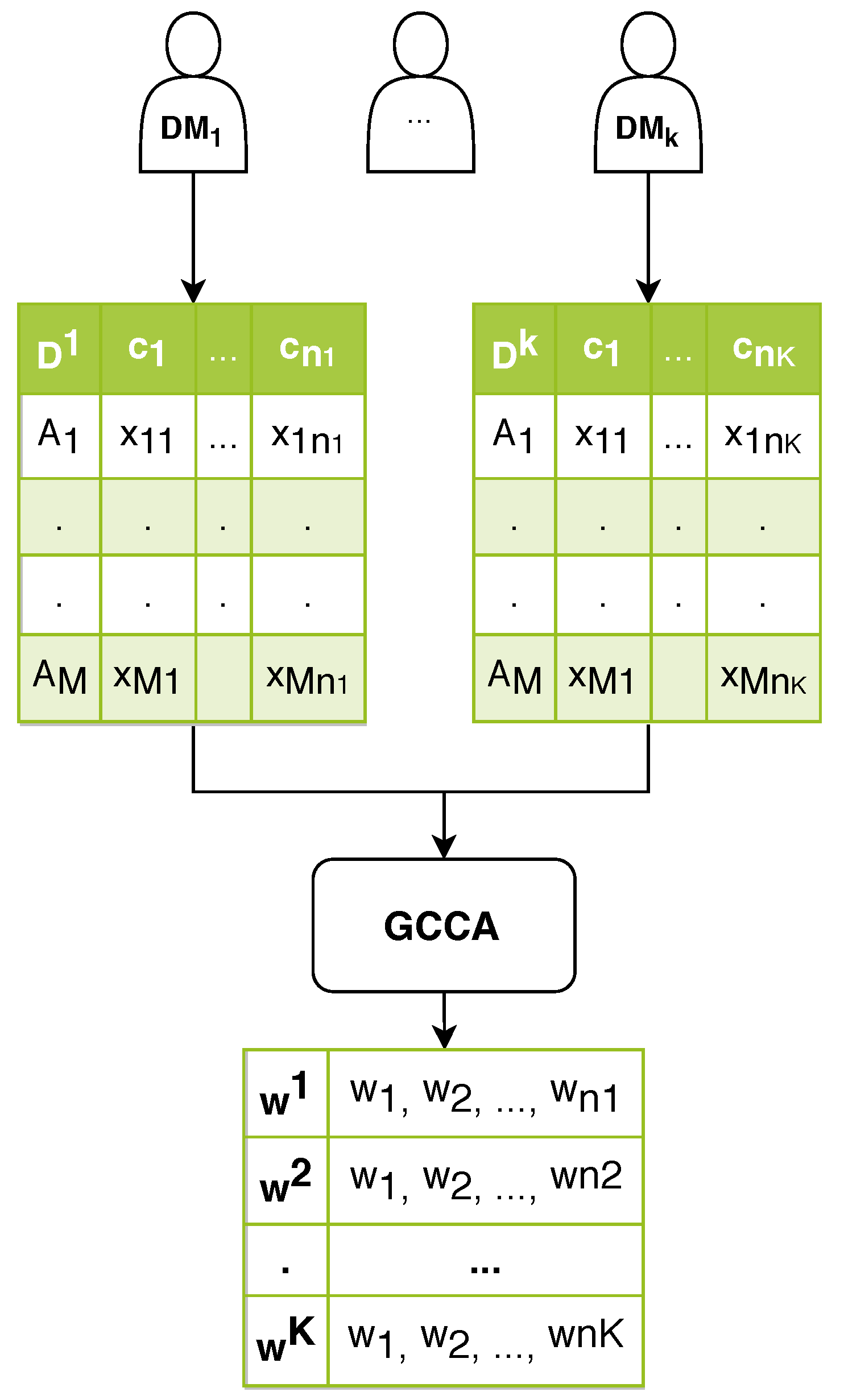
By drawing a parallel between GCCA and MCGDM, one can note that methods pertaining to both areas operate on numerical values arranged in two-dimensional (data/decision) matrices. While, in GCCA, there is a set of data instances (rows) represented by two or more variable sets (columns), in MCGDM one has a set of solution alternatives (rows), each assessed in accordance with two or more sets of criteria (columns). By establishing this correspondence, it is possible to make use of GCCA’s functionalities to automatically compute the values of the criteria weights used in MCGDM.
Assume that K decision matrices are available, with pertaining to the k-th DM, . GCCA is directly applied to all K matrices at once, yielding the criteria weights that are related to each matrix (refer to Figure 1). These weights are the canonical weights that are associated with the first dimension of the canonical space. To bring about the consensus decision between the DMs, CMCGDM employs the same steps of the extended TOPSIS variant proposed by Shih et al. [26] (see Section 2.1), with some minor modifications. More specifically, while the computation of and (Equations (3) and (4)) in the third step now takes into account the positive/negative signs of the canonical weights as calculated by GCCA (i.e., before they are normalized), in the fifth step the computation of and (Equations (5) and (6)) makes use of the normalized weights.
We claim that the above methodology is useful for capturing the intrinsic relationships between the DMs’ beliefs regarding the relative performance of the different alternatives. Usually, the weights of the criteria adopted by all DMs are separately calculated for each DM (sometimes via an unrelated methodology, such as in [52]) and, then, the group consensus is achieved by somehow reconciling the different weights adopted by the different DMs. In the case of CMCGDM, because the canonical weights maximize the correlation between the different decision matrices simultaneously, it is expected that the consensus between the experts can be captured more naturally and effectively, bringing about a more reliable ranking of the available alternatives. In this case, the canonical correlation index can be interpreted as a sort of consensus indicator between the DMs’ opinions.
When considering the more complicated setting where different groups of criteria are used by different DMs, our method can work well, even when the sets of criteria are completely disjoint (that is, with no overlap). Moreover, instead of generating separate rankings of alternatives for all criteria subsets, which are then aggregated to compose the final ranking by solving a specific optimization problem, such as in the approach that was proposed by Fan et al. [21], our methodology seems to be more straightforward, not demanding intermediary rankings for different criteria sets.
Another good property of CMCGDM is that it allows for one to interpret each criterion according to the sign of its associated canonical weight, taking the role played by the other criteria as reference. While positively weighted criteria can be considered as benefit ones, those with negative weights can be regarded as cost criteria.
In order to further clarify this important property, consider a fictitious MCGDM problem that involves four DMs and eight alternatives, each of which is evaluated via five judgment criteria, shared by all DMs. Table 1 and Table 2 show the criteria weights as elicited by GCCA, either before or after normalization is applied. As one can notice, for the first and second DMs, all criteria, except the last one, should be interpreted as of the cost type, since their weights are negative. For the fourth DM, in contrast, the number of benefit criteria is larger. Therefore, the interpretation is contextualized for each DM. Although the non-normalized weights are small in magnitude, they were induced by GCCA so as to maximize the correlation between the DMs’ decision matrices (not shown in this example). After normalization is applied, the magnitude of the criteria weights is rescaled, so that the more relevant ones are more noticeable (they are highlighted in Table 2).
Another good property of CMCGDM is that GCCA is invariant to any affine transformation of the input variables (criteria values), as mentioned before. Besides, like entropy, GCCA is robust against the problem of criteria scaling. By another perspective, the use of GCCA renders our approach flexible enough to allow the dynamic (re)calibration of the criteria weights once the sets of alternatives or criteria change over time. GCCA could be used without modification, even when the number of DMs is allowed to change. However, this important property will not be further explored in this paper and it should be investigated in future work.
We argue that these fine properties are not shared by other popular criteria weighting methods, such as those that are reviewed in Section 2.2. In fact, these methods were not conceived to elicit the weights of different groups of criteria based on the intrinsic relations between the DMs’ preferences (decision matrices). Moreover, as we will show in Section 7, the adopted MCGDM method becomes more resilient to the problem of ranking irregularity [27] when using GCCA in place of the aforementioned criteria weighting methods.
5. Example on Human Resource Selection
To demonstrate the utility of the proposed CMCGDM approach (our implementation uses the Python package Pyrcca [51] for GCCA, which is hosted in http://github.com/gallantlab/pyrcca), we first present in this section the same example considered by Shih et al. [26], which is about the recruitment of an on-line manager by a firm. Subsequently, we compare the performance displayed by the CMCGDM approach with that delivered by the extended TOPSIS version, as originally proposed by Shih et al. [26] (that is, without using GCCA to generate the criteria weights). This is done by considering how resilient each method is to the ranking irregularity problem.
According to the example, the human resource department of the firm coordinates some knowledge tests (namely, language, professional, and safety rule tests), skill tests (namely, professional and computer tests), and interviews (namely, panel and one-on-one interviews) with the candidates. In all, 17 qualified candidates are on the list, whereas four recruiters (DMs) are responsible for conducting the selection. The decision matrix that was used for the decision process is split in Table 3 and Table 4, according to the type of judgment criteria (objective vs subjective). Notice that the criteria sets are the same for all DMs, and all criteria are regarded as of the benefit type. Moreover, all of the DMs share the same score values for the objective criteria, only changing their assessment on the two subjective criteria. In addition, the normalized criteria weights elicited by the DMs themselves (as originally used in [26]) are shown in Table 5, whereas the canonical weights that are generated by GCCA (normalized or not) are displayed in Table 6.
According to Wang and Triantaphyllou [27], an intriguing problem that may happen with different decision-making methods is that of generating disparate outcomes (rankings) when submitted to the same decision problem instance. Consequently, it is natural to raise the question of how to properly assess the performance of such methods. Because it is practically impossible to know which is the best alternative solution for a given decision problem, in [53] some tests capturing different ranking irregularities are discussed as a way for assessing the performance of multi-criteria methods in general:
- Test #1:
- the best alternative selected should not alter when a non-optimal alternative is added or removed from the problem (assuming that the relative importance of each criterion remains unchanged) [54].
- Test #2:
- Test #3:
Table 7 brings the ranking of the alternatives delivered by the extended TOPSIS, as reported in [26], as well as the results of the application of the three ranking irregularity tests that are described above. Table 8 follows the same layout, but it relates to the extended TOPSIS with criteria weights estimated by GCCA (i.e., CMCGDM approach). In both tables, the second and third columns show the new rankings of the alternatives (and their associated scores) that result when an irrelevant alternative is added or removed, respectively, to the alternative set, whereas the last column exhibits the ranking that results from the replacement of a non-optimal alternative by a worse one. Those cases where the transitivity property is violated (Test #3) are indicated by shadowed alternatives.
The extended TOPSIS, using the weights given in Table 5, could pass well Tests #1 and #2, but failed to respect the transitivity requirement, since there is a ranking position change between alternatives A14 and A17 (A4 and A7) when an irrelevant alternative (namely, A1) is duplicated (removed) during the application of Test #1, as one can readily observe from Table 7. On the other hand, the proposed CMCGDM approach could get through all of the three ranking irregularity tests without generating any ranking inconsistencies.
6. Example on Machine Acquisition
In this section, we conduct the same previous analysis on a second example, taken from [21]. In this example, there are different criteria sets that are associated with different DMs. The decision problem relates to the acquisition of a novel machine by a given manufacturing company. There are seven products (alternatives) under analysis by the manufacture department (DM #1) and the financial department (DM #2). The last alternative was introduced by us in order to turn the decision problem a bit more complex. The criteria concerned by DM #1 include : positioning accuracy (mm), : maximum load (kg), : mean time to failure (h), : degree of standardization of parts, : reliable service life (h), and : delivery time (month). The criteria concerned by DM #2 include : price ($) and : down payment ratio (percent), as well as and .
The second, sixth, seventh, and eighth are cost criteria, while the others are benefit criteria. The weights of the criteria that are concerned by DM #1 are , whereas those of the criteria concerned by DM #2 are . The example, as proposed by Fan et al. [21], assumes that such weights were somehow calculated by the DMs themselves.
Table 9 and Table 10 bring the decision matrices that are associated with each DM, respectively, whereas Table 11 and Table 12 bring the results of the application of the three ranking irregularity tests described in the previous section. The layouts of these tables are the same of Table 7 and Table 8. As before, the extended TOPSIS could not keep up well with the transitivity requisite when a mid-ranked alternative (namely, A2) is duplicated. CMCGDM, in turn, could produce rankings showing no inconsistencies according to all ranking irregularity tests.
7. Simulated Cases
In the previous sections, the criteria weights that were used in the comparative analysis were set up either by the DMs themselves or via GCCA. In this section, we enlarge the assessment by also considering the objective criteria weighting methods that are discussed in Section 2.2. The idea is to study, via several simulated cases, how the choice of the weighting method affects the behavior of the extended TOPSIS that was proposed by Shih et al. [26] with respect to the ranking irregularity problem.
The simulations were performed by following the guidelines that were provided in [27,53,56]. According to these authors, the simulations comprise a reasonable expedient to conduct controllable and reproducible experiments in order to have a better understanding of the pros and cons of different multi-criteria decision making methods. By this means, these methods can be deeply assessed by considering different samples and amounts of parameters, numbers of criteria and alternatives, as well as distinct ways to assign weights to the criteria and scores to the alternatives. In our investigation, the main parameters considered along the simulations were the following:
- number of DMs: ;
- number of criteria: 7;
- number of alternatives: ;
- scores of the alternatives: randomly generated by a uniform distribution in the range [0–100];
- criteria weighting approach: GCCA and the methods described in Section 2.2;
- number of trials: 100 for each parameter configuration, thereby yielding 6300 different decision problem instances; and,
- performance criteria: the three irregularity tests described in Section 5.
Table 13 shows the results that were delivered by extended TOPSIS when configured with the different criteria weighting methods (it is worthy reminding that extended TOPSIS using GCCA refers to the CMCGDM approach). The third and fourth columns of this table indicate the number of problem instances (out of 6300) for which the transitivity requirement was violated when an unimportant alternative was inserted or removed, respectively. The fifth column does the same transitivity test, but it refers to those simulation trials where a non-optimal alternative was replaced by a worse one. Conversely, the sixth and seventh columns express the number of cases where the best alternative solution was altered either by adding/removing an irrelevant alternative or by replacing a non-optimal alternative by a worse one. Finally, the last column indicates the aggregated sum of the values in the third, fourth, and fifth columns. As one can notice, using GCCA to elicit the criteria weights has usually achieved better performance than the other contestant methods, lagging behind the statistical variance procedure and CRITIC when the best alternative solutions were altered after adding irrelevant alternatives.
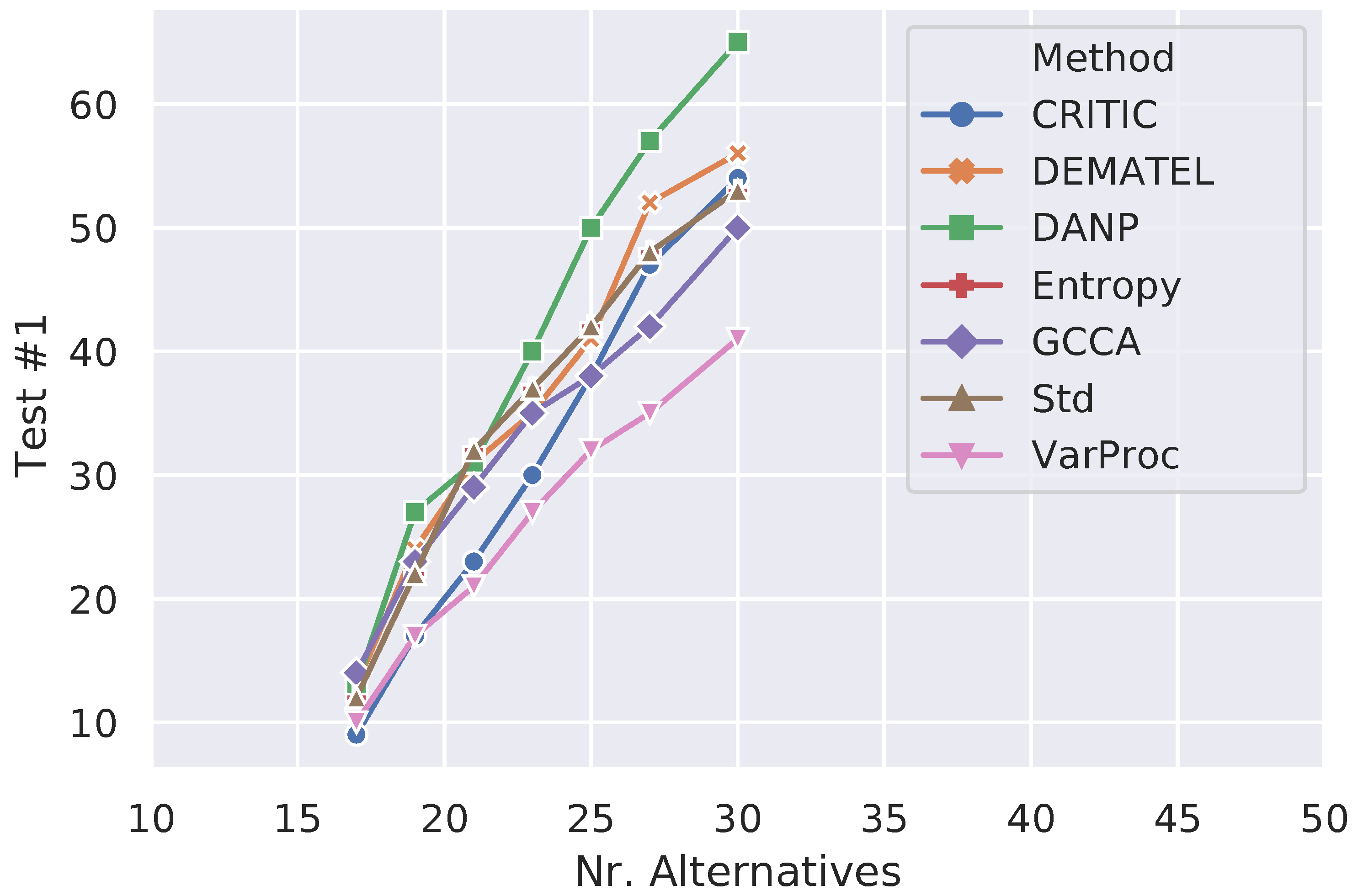
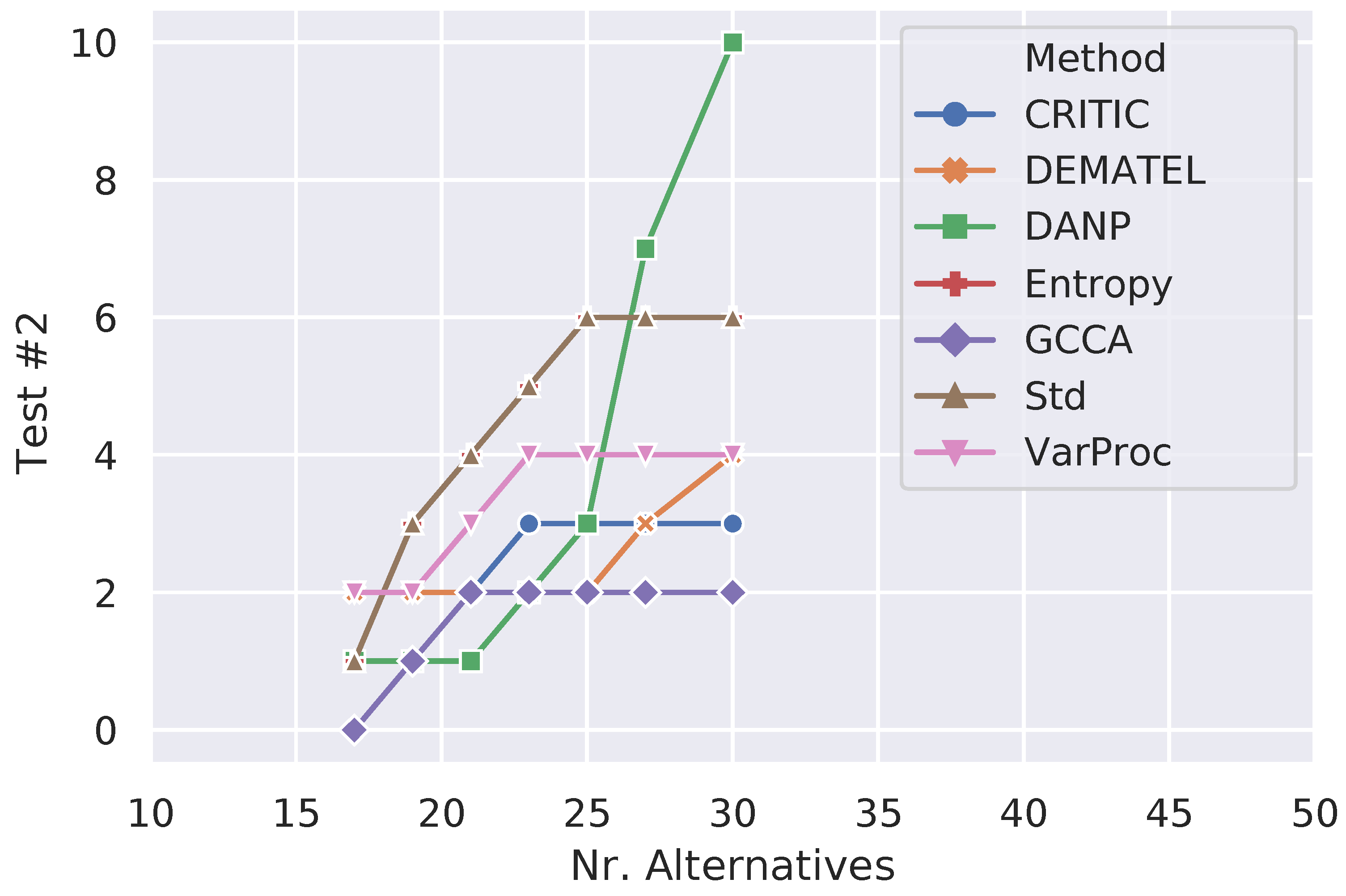
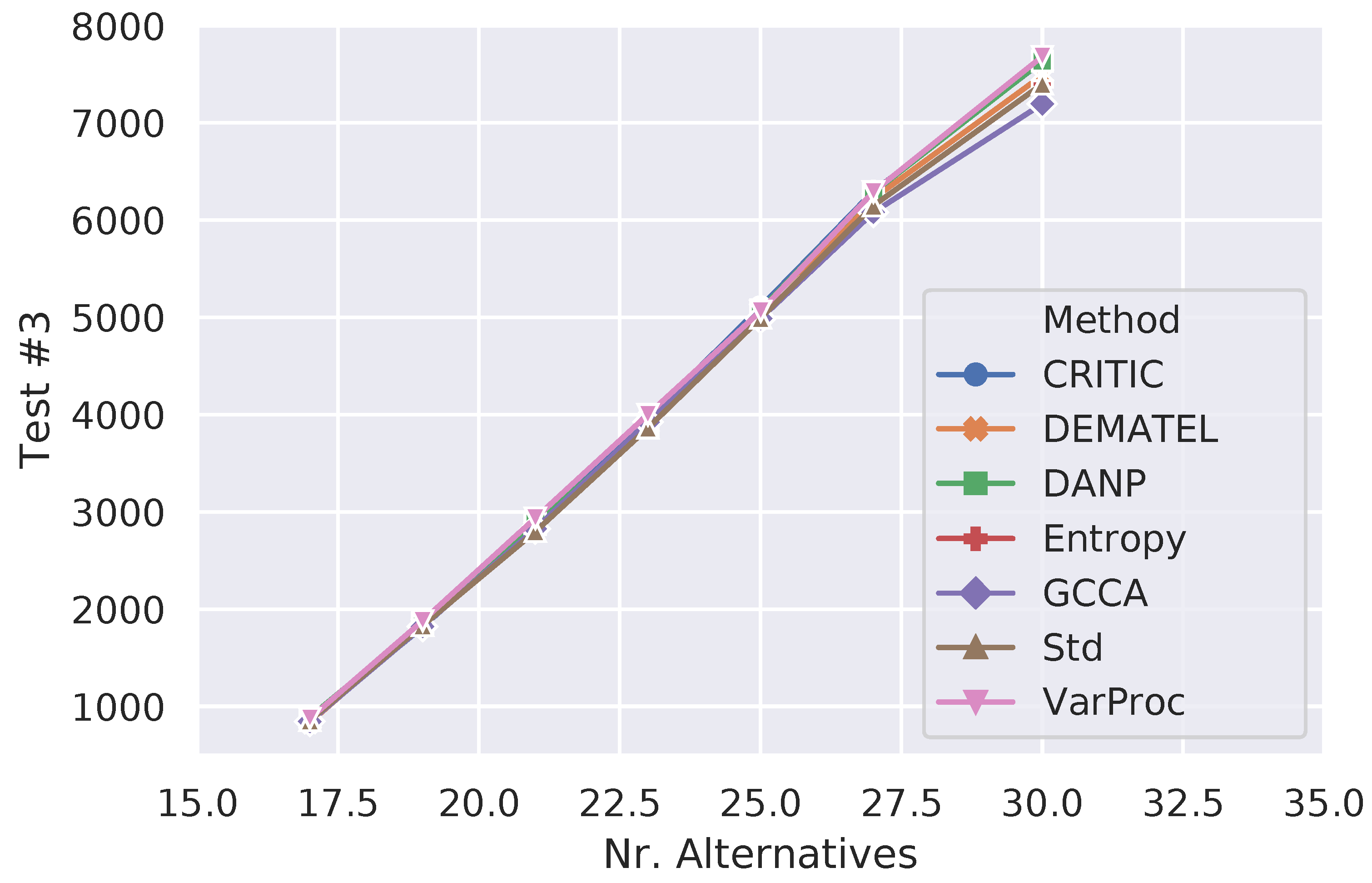
Figure 2, Figure 3 and Figure 4 show how the number of failure cases varied for each type of irregularity test when the number of alternatives increased from 17 (minimum) to 30 (maximum) in order to better understand the performance of the different criteria weighting methods across the simulations. Considering Figure 2 (Test #1), one can notice that GCCA’s overall performance falls short of CRITIC and VarProc, although, after the 25 mark, it is only surpassed by VarProc. While the number of test failures caused by DANP grew up steadily, the increase of this number for GCCA is less accentuated in the range of 25 to 30 alternatives. Regarding Figure 3 (Test #2), the overall performance of GCCA is much better than all other methods and its stability from the 21 mark is remarkable. In general, all methods (except DANP) show a reasonable resilience to the conditions imposed by this test. Finally, Figure 4 informs how the different methods handled the transitivity requirement (Test #3). The values correspond to the aggregated cases, as shown in the last column of Table 13. All methods displayed a similar monotonically increasing behavior in terms of number of failed trials; however, the performance of GCCA was usually better, regardless of the number of alternatives.
8. Final Remarks
In this paper, we introduced a novel GDM approach, CMCGDM, which adopts GCCA to automatically elicit the weights of the (possibly distinct) criteria used by the different DMs. By maximizing the correlation between the DMs’ decision matrices, we argue that the elicited weights can better reflect the consensus between the DMs’ preferences regarding the various alternatives. CMCGDM also makes use of the extended version of TOPSIS conceived by Shih et al. [26], which is specific for MCGDM. We revisited two examples taken from the literature and performed a series of simulations considering popular criteria weighting methods to demonstrate the usefulness of CMCGDM. Overall, the results revealed that CMCGDM is a promising approach, being more resilient to the ranking irregularity problem than the extended TOPSIS without using GCCA.
As future work, we plan to extend CMCGDM to work with other GDM methods available in the literature as well as with uncertain criteria, such as those that involve fuzzy, interval, incomplete, or random values [1,14,57]. We also plan to compare CMCGDM with other methods for eliciting criteria weights, such as CSW-DEA [36,37], nonlinear programming methods [39], and swing-weighting [40]. We shall also investigate the use of GCCA to recalibrate the criteria weights in dynamic settings, particularly in those circumstances where the sets of alternatives or criteria are allowed to change over time [58]. Finally, the use of non-linear versions of CCA (such as those that employ kernels [22]) seems to be a good theme to explore.
Author Contributions
Both authors contributed equally for this work. Both authors have read and agreed to the published version of the manuscript. All authors have read and agreed to the published version of the manuscript.
Funding
This research received no external funding.
Acknowledgments
The first author gratefully acknowledges the financial support given by Banco do Nordeste do Brasil.
Conflicts of Interest
The authors declare no conflict of interest.
References
- Capuano, N.; Chiclana, F.; Fujita, H.; Herrera-Viedma, E.; Loia, V. Fuzzy group decision making with incomplete information guided by social influence. IEEE Trans. Fuzzy Syst. 2018, 26, 1704–1718. [Google Scholar] [CrossRef]
- Liu, W.; Dong, Y.; Chiclana, F.; Cabrerizo, F.; Herrera-Viedma, E. Group decision-making based on heterogeneous preference relations with self-confidence. Fuzzy Optim. Decis. Mak. 2016, 16, 429–447. [Google Scholar] [CrossRef] [Green Version]
- Heravi, G.; Fathi, M.; Faeghi, S. Multi-criteria group decision-making method for optimal selection of sustainable industrial building options focused on petrochemical projects. J. Clean. Prod. 2017, 142, 2999–3013. [Google Scholar] [CrossRef]
- Montajabiha, M. An extended PROMETHE II multi-criteria group decision making technique based on intuitionistic fuzzy logic for sustainable energy planning. Group Decis. Negot. 2015, 25, 221–244. [Google Scholar] [CrossRef]
- Yu, D.; Zhang, W.; Xu, Y. Group decision making under hesitant fuzzy environment with application to personnel evaluation. Knowl. Based Syst. 2013, 52, 1–10. [Google Scholar] [CrossRef]
- Wu, J.; Chiclana, F. A social network analysis trust–consensus based approach to group decision-making problems with interval-valued fuzzy reciprocal preference relations. Knowl. Based Syst. 2014, 59, 97–107. [Google Scholar] [CrossRef] [Green Version]
- Efe, B. An integrated fuzzy multi criteria group decision making approach for ERP system selection. Appl. Soft Comput. 2016, 38, 106–117. [Google Scholar] [CrossRef]
- Kara, S.; Cheikhrouhou, N. A multi criteria group decision making approach for collaborative software selection problem. J. Intell. Fuzzy Syst. 2014, 26, 37–47. [Google Scholar] [CrossRef]
- Liu, Y.; Jin, L.; Zhu, F. A multi-criteria group decision making model for green supplier selection under the ordered weighted hesitant fuzzy environment. Symmetry 2019, 11, 17. [Google Scholar] [CrossRef] [Green Version]
- Wan, S.-P.; Wang, F.; Lin, L.-L.; Dong, J.-Y. An intuitionistic fuzzy linear programming method for logistics outsourcing provider selection. Knowl. Based Syst. 2015, 82, 80–94. [Google Scholar] [CrossRef]
- Zhou, J.; Su, W.; Balezentis, T.; Streimikiene, D. Multiple criteria group decision-making considering symmetry with regards to the positive and negative ideal solutions via the Pythagorean normal cloud model for application to economic decisions. Symmetry 2018, 10, 140. [Google Scholar] [CrossRef] [Green Version]
- Herrera-Viedma, E.; Alonso, S.; Chiclana, F.; Herrera, F. A consensus model for group decision making with incomplete fuzzy preference relations. IEEE Trans. Fuzzy Syst. 2007, 15, 863–877. [Google Scholar] [CrossRef]
- Pérez, I.; Cabrerizo, F.; Herrera-Viedma, E. A mobile decision support system for dynamic group decision-making problems. IEEE Trans. Syst. Man Cybern. Part A Syst. Humans 2010, 40, 1244–1256. [Google Scholar] [CrossRef]
- Lourenzutti, R.; Krohling, R.A. A generalized TOPSIS method for group decision making with heterogeneous information in a dynamic environment. Inf. Sci. 2016, 330, 1–18. [Google Scholar] [CrossRef]
- Luukka, P.; Collan, M.; Fedrizzi, M. A dynamic fuzzy consensus model with random iterative steps. In Proceedings of the 2015 48th Hawaii International Conference on System Sciences, Kauai, HI, USA, 5–8 January 2015; pp. 1474–1482. [Google Scholar]
- Dong, Y.; Chen, X.; Liang, H.; Li, C.-C. Dynamics of linguistic opinion formation in bounded confidence model. Inf. Fusion 2016, 32, 52–61. [Google Scholar] [CrossRef] [Green Version]
- Dong, Y.; Zhang, H.; Herrera-Viedma, E. Consensus reaching model in the complex and dynamic MAGDM problem. Knowl. Based Syst. 2016, 106, 206–219. [Google Scholar] [CrossRef]
- Cabrerizo, F.; Al-Hmouz, R.; Morfeq, A.; Balamash, A.; Martínez, M.; Herrera-Viedma, E. Soft consensus measures in group decision making using unbalanced fuzzy linguistic information. Soft Comput. 2017, 21, 3037–3050. [Google Scholar] [CrossRef]
- Dong, Q.; Cooper, O. A peer-to-peer dynamic adaptive consensus reaching model for the group AHP decision making. Eur. J. Oper. Res. 2016, 250, 521–530. [Google Scholar] [CrossRef]
- Tervonen, T.; Figueira, J.; Lahdelma, R.; Dias, J.; Salminen, P. A stochastic method for robustness analysis in sorting problems. Eur. J. Oper. Res. 2009, 192, 236–242. [Google Scholar] [CrossRef]
- Fan, Z.-P.; Li, M.-Y.; Liu, Y.; You, T.-H. A method for multicriteria group decision making with different evaluation criterion sets. Math. Probl. Eng. 2018, 2018, 7189451. [Google Scholar] [CrossRef]
- Uurtio, V.; Monteiro, J.M.; Kandola, J.; Shawe-Taylor, J.; Fernandez-Reyes, D.; Rousu, J. A tutorial on canonical correlation methods. ACM Comput. Surv. 2017, 50, 95. [Google Scholar] [CrossRef] [Green Version]
- McGarigal, K.; Cushman, S.; Stafford, S. Multivariate Statistics for Wildlife Ecology Research; Springer: New York, NY, USA, 2000. [Google Scholar]
- Kettenring, J.R. Canonical analysis of several sets of variables. Biometrika 1971, 58, 433–451. [Google Scholar] [CrossRef]
- Hwang, C.; Yoon, K. Multiple Attribute Decision Making: Methods and Applications—A State-of-the-Art Survey; Springer: Berlin/Heidelberg, Germany, 1981. [Google Scholar]
- Shih, H.-S.; Shyur, H.-J.; Lee, E.S. An extension of TOPSIS for group decision making. Math. Comput. Model. 2007, 45, 801–813. [Google Scholar] [CrossRef]
- Wang, X.; Triantaphyllou, E. Ranking irregularities when evaluating alternatives by using some ELECTRE methods. Omega 2008, 36, 45–63. [Google Scholar] [CrossRef]
- Banihabib, M.; Hashemi-Madani, F.; Forghani, A. Comparison of compensatory and non-compensatory multi criteria decision making models in water resources strategic management. Water Resour. Manag. 2017, 31, 3745–3759. [Google Scholar] [CrossRef]
- Papathanasiou, J.; Ploskas, N. Multiple Criteria Decision Aid—Methods, Examples and Python Implementations; Springer: Cham, Switzerland, 2018. [Google Scholar]
- Pöyhönen, M.; Hämäläinen, R.P. On the convergence of multiattribute weighting methods. Eur. J. Oper. Res. 2001, 129, 569–585. [Google Scholar] [CrossRef] [Green Version]
- Deng, H.; Yeh, C.-H.; Willis, R.J. Inter-company comparison using modified TOPSIS with objective weights. Comput. Oper. Res. 2000, 27, 963–973. [Google Scholar] [CrossRef]
- Jahan, A.; Mustapha, F.; Sapuan, S.; Ismail, M.; Bahraminasab, M. A framework for weighting of criteria in ranking stage of material selection process. Int. J. Adv. Manuf. Technol. 2012, 58, 411–420. [Google Scholar] [CrossRef]
- Diakoulaki, D.; Mavrotas, G.; Papayannakis, L. Determining objective weights in multiple criteria problems: The critic method. Comput. Oper. Res. 1995, 22, 763–770. [Google Scholar] [CrossRef]
- Gabus, A. DEMATEL, Innovative Methods, Report No. 2 Structural Analysis of the World Problematique; Battelle Geneva Research Institute: Geneva, Switzerland, 1974. [Google Scholar]
- Yang, Y.-P.O.; Leu, J.-D.; Tzeng, G.-H. A novel hybrid MCDM model combined with DEMATEL and ANP with applications. Int. J. Oper. Res. 2008, 5, 160–168. [Google Scholar]
- Ramezani-Tarkhorani, S.; Khodabakhshi, M.; Mehrabian, S.; Nuri-Bahmani, F. Ranking decision-making units using common weights in DEA. Appl. Math. Model. 2014, 38, 3890–3896. [Google Scholar] [CrossRef]
- Hammami, H.; Ngo, T.; Tripe, D.; Vo, D.-T. Ranking with a Euclidean common set of weights in data envelopment analysis: With application to the Eurozone banking sector. Ann. Oper. Res. 2020. accepted. [Google Scholar]
- Ramón, N.; Ruiz, J.L.; Sirvent, I. Common sets of weights as summaries of DEA profiles of weights: With an application to the ranking of professional tennis players. Expert Syst. Appl. 2012, 39, 4882–4889. [Google Scholar] [CrossRef]
- Movafaghpour, M. An efficient nonlinear programming method for eliciting preference weights of incomplete comparisons. J. Appl. Res. Ind. Eng. 2019, 6, 131–138. [Google Scholar]
- Parnell, G.S.; Trainor, T.E. 2.3.1 using the swing weight matrix to weight multiple objectives. INCOSE Int. Symp. 2009, 19, 283–298. [Google Scholar] [CrossRef]
- Wang, J.-J.; Jing, Y.-Y.; Zhang, C.-F.; Zhao, J.-H. Review on multi-criteria decision analysis aid in sustainable energy decision-making. Renew. Sustain. Energy Rev. 2009, 13, 2263–2278. [Google Scholar] [CrossRef]
- Kobryń, A. DEMATEL as a weighting method in multi-criteria decision analysis. Mult. Criteria Decis. Mak. 2018, 4, 12. [Google Scholar] [CrossRef] [Green Version]
- Dytczak, M.; Ginda, G. DEMATEL-based ranking approaches. Cent. Eur. Rev. Econ. Manag. 2016, 16, 191–202. [Google Scholar] [CrossRef]
- Zhu, B.-W.; Zhang, J.-R.; Tzeng, G.-H.; Huang, S.-L.; Xiong, L. Public open space development for elderly people by using the danp-v model to establish continuous improvement strategies towards a sustainable and healthy aging society. Sustainability 2017, 9, 420. [Google Scholar] [CrossRef] [Green Version]
- Gabus, A.; Fontela, E. World Problems an Invitation to Further thought within the Frame-Work of DEMATEL; Battelle Geneva Research Institute: Geneva, Switzerland, 1972. [Google Scholar]
- Saaty, T.L. Decision Making with Dependence and Feedback: The Analytic Network Process; RWS: Singapore, 1996. [Google Scholar]
- Fontela, E.; Gabus, A. The DEMATEL Observer; Battelle Geneva Research Institute: Geneva, Switzerland, 1976. [Google Scholar]
- Manly, B.F.; Alberto, J.A.N. Multivariate Statistical Methods: A Primer, 4th ed.; Chapman and Hall/CRC: Boca Raton, FL, USA, 2016. [Google Scholar]
- Meloun, M.; Militký, J. Statistical Data Analysis—A Practical Guide; Woodhead Publishing: New Delhi, India, 2011. [Google Scholar]
- Donner, R.; Reiter, M.; Langs, G.; Peloschek, P.; Bischof, H. Fast active appearance model search using Canonical Correlation Analysis. IEEE Trans. Pattern Anal. Mach. Intell. 2006, 28, 1690–1694. [Google Scholar] [CrossRef] [Green Version]
- Bilenko, N.Y.; Gallant, J.L. Pyrcca: Regularized kernel canonical correlation analysis in python and its applications to neuroimaging. Front. Neuroinform. 2016, 10, 49. [Google Scholar] [CrossRef] [PubMed] [Green Version]
- Shih, H.-S.; Wang, C.-H.; Lee, E. A multiattribute GDSS for aiding problem-solving. Math. Comput. Model. 2004, 39, 1397–1412. [Google Scholar] [CrossRef]
- Triantaphyllou, E. Multi-Criteria Decision Making Methods: A Comparative Study; Springer: Boston, MA, USA, 2013. [Google Scholar]
- Cinelli, M.; Coles, S.R.; Kirwan, K. Analysis of the potentials of multi criteria decision analysis methods to conduct sustainability assessment. Ecol. Indic. 2014, 46, 138–148. [Google Scholar] [CrossRef] [Green Version]
- Triantaphyllou, E. Two new cases of rank reversals when the AHP and some of its additive variants are used that do not occur with the multiplicative AHP. J. Multi Criteria Decis. Anal. 2001, 10, 11–25. [Google Scholar] [CrossRef]
- Aires, R.; Ferreira, L. A new approach to avoid rank reversal cases in the TOPSIS method. Comput. Ind. Eng. 2019, 132, 84–97. [Google Scholar] [CrossRef]
- Celik, E.; Gul, M.; Aydin, N.; Gumus, A.T.; Guneri, A.F.A. Comprehensive review of multi criteria decision making approaches based on interval type-2 fuzzy sets. Knowl. Based Syst. 2015, 85, 329–341. [Google Scholar] [CrossRef]
- Campanella, G.; Ribeiro, R. A framework for dynamic multiple-criteria decision making. Decis. Support Syst. 2011, 52, 52–60. [Google Scholar] [CrossRef]
Figure 1.
Steps of the proposed canonical multi-criteria group decision making (CMCGDM) approach.

Figure 2.
Performance of the different criteria weighting methods on Test #1.

Figure 3.
Performance of the different criteria weighting methods on Test #2.

Figure 4.
Performance of the different criteria weighting methods on Test #3.


Table 1.
Fictitious multi-criteria group decision making (MCGDM) problem—non-normalized generalized version of canonical correlation analysis (GCCA) weights.
Table 1.
Fictitious multi-criteria group decision making (MCGDM) problem—non-normalized generalized version of canonical correlation analysis (GCCA) weights.
| Criteria | DM1 | DM2 | DM3 | DM4 |
|---|---|---|---|---|
| C1 | −0.0116 | −0.0081 | −0.0105 | 0.0071 |
| C2 | −0.0122 | −0.0063 | 0.0037 | 0.0033 |
| C3 | −0.0049 | −0.0123 | −0.0053 | −0.0184 |
| C4 | −0.0123 | −0.0132 | 0.0015 | −0.0167 |
| C5 | 0.0148 | 0.0157 | −0.0229 | 0.0004 |
Table 2.
Fictitious MCGDM problem—normalized GCCA weights.
| Criteria | DM1 | DM2 | DM3 | DM4 |
|---|---|---|---|---|
| C1 | 0.0218 | 0.1227 | 0.1528 | 0.3769 |
| C2 | 0.0025 | 0.1652 | 0.3284 | 0.3201 |
| C3 | 0.2107 | 0.0206 | 0.2173 | 0.0000 |
| C4 | 0.0000 | 0.0000 | 0.3014 | 0.0250 |
| C5 | 0.7650 | 0.6915 | 0.0000 | 0.2780 |
Table 3.
Decision matrix (objective criteria) for the first example, adapted from ([26] [Table 6a]).
Table 3.
Decision matrix (objective criteria) for the first example, adapted from ([26] [Table 6a]).
| No. | Candidates | Objective Criteria | ||||
|---|---|---|---|---|---|---|
| Knowledge Tests | Skill Tests | |||||
| Language Test | Professional Test | Safety Rule Test | Professional Skills | Computer Skills | ||
| 1 | James B. Wang | 80 | 70 | 87 | 77 | 76 |
| 2 | Carol L. Lee | 85 | 65 | 76 | 80 | 75 |
| 3 | Kenney C. Wu | 78 | 90 | 72 | 80 | 75 |
| 4 | Robert M. Liang | 75 | 84 | 69 | 85 | 65 |
| 5 | Sophia M. Cheng | 84 | 67 | 60 | 75 | 85 |
| 6 | Lily M. Pai | 85 | 78 | 82 | 81 | 79 |
| 7 | Abon C. Hsieh | 77 | 83 | 74 | 70 | 71 |
| 8 | Frank K. Yang | 78 | 82 | 72 | 80 | 78 |
| 9 | Ted C. Yang | 85 | 90 | 80 | 88 | 90 |
| 10 | Sue B. Ho | 89 | 75 | 79 | 67 | 77 |
| 11 | Vincent C. Chen | 65 | 55 | 68 | 62 | 70 |
| 12 | Rosemary I. Lin | 70 | 64 | 65 | 65 | 60 |
| 13 | Ruby J. Huang | 95 | 80 | 70 | 75 | 70 |
| 14 | George K. Wu | 70 | 80 | 79 | 80 | 85 |
| 15 | Philip C. Tsai | 60 | 78 | 87 | 70 | 66 |
| 16 | Michael S. Liao | 92 | 85 | 88 | 90 | 85 |
| 17 | Michelle C. Lin | 86 | 87 | 80 | 70 | 72 |
Table 4.
Decision matrix (subjective criteria) for the first example, adapted from ([26] [Table 6b]).
Table 4.
Decision matrix (subjective criteria) for the first example, adapted from ([26] [Table 6b]).
| No. | Subjective Criteria | |||||||
|---|---|---|---|---|---|---|---|---|
| DM #1 | DM #2 | DM #3 | DM #4 | |||||
| Panel Interview | 1-on-1 Interview | Panel Interview | 1-on-1 Interview | Panel Interview | 1-on-1 Interview | Panel Interview | 1-on-1 Interview | |
| 1 | 80 | 75 | 85 | 80 | 75 | 70 | 90 | 85 |
| 2 | 65 | 75 | 60 | 70 | 70 | 77 | 60 | 70 |
| 3 | 90 | 85 | 80 | 85 | 80 | 90 | 90 | 95 |
| 4 | 65 | 70 | 55 | 60 | 68 | 72 | 62 | 72 |
| 5 | 75 | 80 | 75 | 80 | 50 | 55 | 70 | 75 |
| 6 | 80 | 80 | 75 | 85 | 77 | 82 | 75 | 75 |
| 7 | 65 | 70 | 70 | 60 | 65 | 72 | 67 | 75 |
| 8 | 70 | 60 | 75 | 65 | 75 | 67 | 82 | 85 |
| 9 | 80 | 85 | 95 | 85 | 90 | 85 | 90 | 92 |
| 10 | 70 | 75 | 75 | 80 | 68 | 78 | 65 | 70 |
| 11 | 50 | 60 | 62 | 65 | 60 | 65 | 65 | 70 |
| 12 | 60 | 65 | 65 | 75 | 50 | 60 | 45 | 50 |
| 13 | 75 | 75 | 80 | 80 | 65 | 75 | 70 | 75 |
| 14 | 80 | 70 | 75 | 72 | 80 | 70 | 75 | 75 |
| 15 | 70 | 65 | 75 | 70 | 65 | 70 | 60 | 65 |
| 16 | 90 | 95 | 92 | 90 | 85 | 80 | 88 | 90 |
| 17 | 80 | 85 | 70 | 75 | 75 | 80 | 70 | 75 |
Table 5.
Original criteria weights for the first example, adapted from ([26] [Table 6b]).
Table 5.
Original criteria weights for the first example, adapted from ([26] [Table 6b]).
| No. | Criteria | The Weights of the Group | |||
|---|---|---|---|---|---|
| DM #1 | DM #2 | DM #3 | DM #4 | ||
| Knowledge tests | |||||
| 1 | Language test | 0.066 | 0.042 | 0.060 | 0.047 |
| 2 | Professional test | 0.196 | 0.112 | 0.134 | 0.109 |
| 3 | Safety rule test | 0.066 | 0.082 | 0.051 | 0.037 |
| Skill tests | |||||
| 4 | Professional skills | 0.130 | 0.176 | 0.167 | 0.133 |
| 5 | Computer skills | 0.130 | 0.118 | 0.100 | 0.081 |
| Interviews | |||||
| 6 | Panel interview | 0.216 | 0.215 | 0.203 | 0.267 |
| 7 | 1-on-1 interview | 0.196 | 0.215 | 0.285 | 0.326 |
| Sum | 1 | 1 | 1 | 1 | |
Table 6.
Criteria weights (non-normalized values in parentheses) for the first example, as elicited by GCCA.
Table 6.
Criteria weights (non-normalized values in parentheses) for the first example, as elicited by GCCA.
| No. | Criteria | The Weights of the Group | |||
|---|---|---|---|---|---|
| DM #1 | DM #2 | DM #3 | DM #4 | ||
| Knowledge tests | |||||
| 1 | Language test | 0.2665 (0.0003) | 0.1661 (−0.0001) | 0.1668 (0.0014) | 0.1251 (0.0005) |
| 2 | Professional test | 0.0000 (−0.0119) | 0.0383 (−0.0092) | 0.0156 (−0.0107) | 0.0104 (−0.0109) |
| 3 | Safety rule test | 0.2368 (−0.0011) | 0.0626 (−0.0075) | 0.1927 (0.0035) | 0.1827 (0.0062) |
| Skill tests | |||||
| 4 | Professional skills | 0.2057 (−0.0025) | 0.1885 (0.0015) | 0.0875 (−0.0049) | 0.1470 (0.0027) |
| 5 | Computer skills | 0.0503 (−0.0096) | 0.2984 (0.0093) | 0.0798 (−0.0056) | 0.2033 (0.0083) |
| Interviews | |||||
| 6 | Panel interview | 0.1266 (−0.0061) | 0.2101 (0.0030) | 0.2985 (0.0119) | 0.2157 (0.0095) |
| 7 | 1-on-1 interview | 0.1142 (−0.0067) | 0.0360 (−0.0094) | 0.1590 (0.0008) | 0.1158 (−0.0004) |
| Sum | 1 | 1 | 1 | 1 | |
Table 7.
Assessment of the extended TOPSIS [26] on the ranking irregularity tests—first example.
Table 7.
Assessment of the extended TOPSIS [26] on the ranking irregularity tests—first example.
| Extended TOPSIS | Test #1–Addition | Test #1–Removal | Test #2 | ||||
|---|---|---|---|---|---|---|---|
| Rank | Score | Rank | Score | Rank | Score | Rank | Score |
| A16 | 0.8960 | A16 | 0.8956 | A16 | 0.8963 | A16 | 0.8960 |
| A9 | 0.8797 | A9 | 0.8797 | A9 | 0.8797 | A9 | 0.8797 |
| A3 | 0.7860 | A3 | 0.7862 | A3 | 0.7859 | A3 | 0.7860 |
| A6 | 0.6611 | A6 | 0.6611 | A6 | 0.6611 | A6 | 0.6611 |
| A1 | 0.6272 | A1 | 0.6259 | A14 | 0.5925 | A14 | 0.5924 |
| A14 | 0.5924 | A1 | 0.6259 | A17 | 0.5915 | A17 | 0.5919 |
| A17 | 0.5920 | A17 | 0.5925 | A8 | 0.5700 | A8 | 0.5701 |
| A8 | 0.5701 | A14 | 0.5924 | A13 | 0.5565 | A13 | 0.5568 |
| A13 | 0.5568 | A8 | 0.5701 | A10 | 0.5079 | A10 | 0.5080 |
| A10 | 0.5080 | A13 | 0.5571 | A5 | 0.4660 | A5 | 0.4660 |
| A5 | 0.4660 | A10 | 0.5082 | A7 | 0.4516 | A4 | 0.4524 |
| A4 | 0.4527 | A5 | 0.4659 | A4 | 0.4514 | A7 | 0.4522 |
| A7 | 0.4523 | A4 | 0.4538 | A2 | 0.4401 | A2 | 0.4404 |
| A2 | 0.4404 | A7 | 0.4530 | A15 | 0.4092 | A1 | 0.4224 |
| A15 | 0.4091 | A2 | 0.4406 | A11 | 0.2101 | A15 | 0.4091 |
| A11 | 0.2097 | A15 | 0.4091 | A12 | 0.1673 | A11 | 0.2097 |
| A12 | 0.1678 | A11 | 0.2093 | ---- | ---- | A12 | 0.1677 |
| ---- | ---- | A12 | 0.1682 | ---- | ---- | ---- | ---- |
Table 8.
Assessment of the CMCGDM approach on the ranking irregularity tests–first example.
| CMCGDM | Test #1–Addition | Test #1–Removal | Test #2 | ||||
|---|---|---|---|---|---|---|---|
| Rank | Score | Rank | Score | Rank | Score | Rank | Score |
| A16 | 0.9016 | A16 | 0.9013 | A16 | 0.9018 | A16 | 0.9016 |
| A9 | 0.8797 | A9 | 0.8799 | A9 | 0.8794 | A9 | 0.8796 |
| A3 | 0.7230 | A3 | 0.7231 | A3 | 0.7228 | A3 | 0.7230 |
| A6 | 0.6720 | A6 | 0.6719 | A6 | 0.6722 | A6 | 0.6721 |
| A14 | 0.6608 | A14 | 0.6608 | A14 | 0.6608 | A14 | 0.6608 |
| A1 | 0.5964 | A1 | 0.5954 | A8 | 0.5854 | A8 | 0.5855 |
| A8 | 0.5855 | A1 | 0.5954 | A5 | 0.5491 | A5 | 0.5495 |
| A5 | 0.5495 | A8 | 0.5855 | A2 | 0.5170 | A2 | 0.5173 |
| A2 | 0.5173 | A5 | 0.5499 | A17 | 0.4813 | A17 | 0.4811 |
| A17 | 0.4811 | A2 | 0.5176 | A13 | 0.4778 | A13 | 0.4779 |
| A13 | 0.4779 | A17 | 0.4810 | A4 | 0.4699 | A4 | 0.4705 |
| A4 | 0.4706 | A13 | 0.4781 | A10 | 0.4634 | A10 | 0.4632 |
| A10 | 0.4632 | A4 | 0.4713 | A7 | 0.3956 | A7 | 0.3957 |
| A7 | 0.3957 | A10 | 0.4630 | A15 | 0.3627 | A1 | 0.3627 |
| A15 | 0.3620 | A7 | 0.3958 | A11 | 0.2259 | A15 | 0.3621 |
| A11 | 0.2254 | A15 | 0.3615 | A12 | 0.1408 | A11 | 0.2255 |
| A12 | 0.1409 | A11 | 0.2250 | ---- | ---- | A12 | 0.1409 |
| ---- | ---- | A12 | 0.1410 | ---- | ---- | ---- | ---- |
Table 9.
Decision matrix associated with DM #1 for the second example, adapted from ([21] [Table 2]).
Table 9.
Decision matrix associated with DM #1 for the second example, adapted from ([21] [Table 2]).
| C1 | C2 | C3 | C4 | C5 | C6 | |
|---|---|---|---|---|---|---|
| A1 | 0.05 | 500 | 850 | 8.6 | 30,500 | 1.5 |
| A2 | 0.01 | 550 | 925 | 8.2 | 26,500 | 2.0 |
| A3 | 0.008 | 600 | 960 | 9.0 | 28,500 | 3.0 |
| A4 | 0.008 | 450 | 720 | 9.2 | 25,800 | 2.0 |
| A5 | 0.015 | 400 | 650 | 8.0 | 24,000 | 1.5 |
| A6 | 0.012 | 480 | 710 | 8.4 | 23,500 | 1.0 |
| A7 | 0.017 | 505 | 691 | 8.0 | 30,100 | 1.3 |
Table 10.
Decision matrix associated with DM #2 for the second example, adapted from ([21] [Table 2]).
Table 10.
Decision matrix associated with DM #2 for the second example, adapted from ([21] [Table 2]).
| C5 | C6 | C7 | C8 | |
|---|---|---|---|---|
| A1 | 30,500 | 1.5 | 530,000 | 50 |
| A2 | 26,500 | 2.0 | 420,000 | 40 |
| A3 | 28,500 | 3.0 | 450,000 | 35 |
| A4 | 25,800 | 2.0 | 480,000 | 40 |
| A5 | 24,000 | 1.5 | 380,000 | 30 |
| A6 | 23,500 | 1.0 | 40,000 | 60 |
| A7 | 30,100 | 1.3 | 392,000 | 57 |
Table 11.
Assessment of the extended TOPSIS [26] on the ranking irregularity tests—second example.
Table 11.
Assessment of the extended TOPSIS [26] on the ranking irregularity tests—second example.
| Extended TOPSIS | Test #1–Addition | Test #1–Removal | Test #2 | ||||
|---|---|---|---|---|---|---|---|
| Rank | Score | Rank | Score | Rank | Score | Rank | Score |
| A1 | 1.0000 | A1 | 1.0000 | A1 | 1.0000 | A1 | 1.0000 |
| A3 | 0.5892 | A3 | 0.5816 | A3 | 0.5984 | A3 | 0.5908 |
| A4 | 0.5265 | A4 | 0.5189 | A4 | 0.5357 | A4 | 0.5281 |
| A2 | 0.4741 | A7 | 0.4682 | A7 | 0.4704 | A7 | 0.4694 |
| A7 | 0.4691 | A2 | 0.4667 | A5 | 0.4011 | A5 | 0.4004 |
| A5 | 0.4002 | A2 | 0.4667 | A6 | 0.0000 | A2 | 0.3748 |
| A6 | 0.0000 | A5 | 0.3996 | ---- | ---- | A6 | 0.0000 |
| ---- | ---- | A6 | 0.0000 | ---- | ---- | ---- | ---- |
Table 12.
Assessment of the CMCGDM approach on the ranking irregularity tests–second example.
| CMCGDM | Test #1–Addition | Test #1–Removal | Test #2 | ||||
|---|---|---|---|---|---|---|---|
| Rank | Score | Rank | Score | Rank | Score | Rank | Score |
| A3 | 0.8455 | A3 | 0.8425 | A3 | 0.8521 | A3 | 0.8478 |
| A4 | 0.5798 | A4 | 0.5784 | A4 | 0.5800 | A4 | 0.5798 |
| A2 | 0.5582 | A2 | 0.5581 | A1 | 0.4529 | A2 | 0.4631 |
| A1 | 0.4578 | A2 | 0.5581 | A5 | 0.3574 | A1 | 0.4577 |
| A5 | 0.3600 | A1 | 0.4627 | A7 | 0.2919 | A5 | 0.3581 |
| A7 | 0.2965 | A5 | 0.3581 | A6 | 0.0000 | A7 | 0.2936 |
| A6 | 0.0000 | A7 | 0.2942 | ---- | ---- | A6 | 0.0000 |
| ---- | ---- | A6 | 0.0000 | ---- | ---- | ---- | ---- |
Table 13.
Assessment of the different criteria weighting methods on the ranking irregularity tests—simulated cases.
Table 13.
Assessment of the different criteria weighting methods on the ranking irregularity tests—simulated cases.
| Test #3 | Test #3 | Test #3 | |||||
|---|---|---|---|---|---|---|---|
| Dist. | Method | Addition | Removal | Replacement | Test #1 | Test #2 | Total Test #3 |
| uniform | GCCA | 11,737 | 13,226 | 2727 | 231 | 11 | 27,690 |
| Entropy | 12,504 | 12,753 | 2640 | 246 | 31 | 27,897 | |
| Std | 12,504 | 12,753 | 2640 | 246 | 31 | 27,897 | |
| DEMATEL | 12,741 | 12,837 | 2626 | 252 | 17 | 28,204 | |
| DEMATEL-ANP | 12,145 | 13,592 | 2766 | 283 | 25 | 28,503 | |
| CRITIC | 12,411 | 13,276 | 2869 | 218 | 16 | 28,556 | |
| VarProc | 12,366 | 13,313 | 3059 | 183 | 23 | 28,738 |
Note: VarProc refers to the statistical variance procedure; Std refers to the standard deviation method.
© 2020 by the authors. Licensee MDPI, Basel, Switzerland. This article is an open access article distributed under the terms and conditions of the Creative Commons Attribution (CC BY) license (http://creativecommons.org/licenses/by/4.0/).
Share and Cite
MDPI and ACS Style
Santos, F.J.d.; Coelho, A.L.V. Eliciting Correlated Weights for Multi-Criteria Group Decision Making with Generalized Canonical Correlation Analysis. Symmetry 2020, 12, 1612. https://0-doi-org.brum.beds.ac.uk/10.3390/sym12101612
AMA Style
Santos FJd, Coelho ALV. Eliciting Correlated Weights for Multi-Criteria Group Decision Making with Generalized Canonical Correlation Analysis. Symmetry. 2020; 12(10):1612. https://0-doi-org.brum.beds.ac.uk/10.3390/sym12101612
Chicago/Turabian StyleSantos, Francisco J. dos, and André L. V. Coelho. 2020. "Eliciting Correlated Weights for Multi-Criteria Group Decision Making with Generalized Canonical Correlation Analysis" Symmetry 12, no. 10: 1612. https://0-doi-org.brum.beds.ac.uk/10.3390/sym12101612
Note that from the first issue of 2016, this journal uses article numbers instead of page numbers. See further details here.