Article

Using Behavioral Instability to Investigate Behavioral Reaction Norms in Captive Animals: Theoretical Implications and Future Perspectives

by
Anne Cathrine Linder
1,†,
Anika Gottschalk
1,†,
Henriette Lyhne
1,†,
Marie Gade Langbak
1,
Trine Hammer Jensen
2 and
Cino Pertoldi
1,2,*
1
Department of Chemistry and Bioscience, Aalborg University, Fredrik Bajers Vej 7H, DK-9000 Aalborg, Denmark
2
Department of Zoology, Aalborg Zoo, Mølleparkvej 63, DK-9000 Aalborg, Denmark
*
Author to whom correspondence should be addressed.
The three authors contributed equally.
Submission received: 9 March 2020 / Revised: 26 March 2020 / Accepted: 2 April 2020 / Published: 10 April 2020

Abstract

:
Behavioral instability is a concept used for indicating environmental stress based on behavioral traits. This study investigates the possibility of using behavioral instability as a tool for assessing behavioral reaction norms in captive animals. The understanding of personality in captive animals can be a useful tool in the development of enrichment programs in order to improve animal welfare. In this study, a case study examined how olfactory stimuli affected the behavior of two polar bears Ursus maritimus in captivity. Using continuous focal sampling throughout the day, it was found that for many behaviors, the individuals responded differently to stimuli, indicating that there was a difference in behavioral reaction norms. This is shown using multiple approaches. One approach used traditional methods for behavioral analyses, and the other approach used the concept of behavioral instability as a new quantitative method. This study demonstrates the utility of behavioral instability as a new quantitative method for investigating behavioral reaction norms, expanding the possibility of comparing behavioral responses between species. Moreover, it is shown that outliers—that cause asymmetric distributions—should not be removed in behavioral analysis, without careful consideration. In conclusion, the theoretical implications and future perspectives of behavioral instability are discussed.

1. Introduction

It has been shown for several species that conspecifics have different behavioral reaction norms [1,2,3]. These different behavioral reaction norms are expressed by consistent behavioral responses under various conditions that can vary in different ways, for example, population density, stress and enrichment [2,4,5]. A behavioral reaction norm is a set of behavioral phenotypes that a single individual produces in a specified set of environments [6]. The behavioral responses of an animal can influence its welfare, as these responses can vary between individuals; that is, an environmental condition may be well tolerated by one individual, but not by another [7]. Stereotypic behavior is described as a repetitive motion with no apparent purpose and has generally been shown to be a sign of stress, due to its correlation with increased corticoid levels, thus making stereotypy an indication of poor welfare [8,9].
Several studies have shown that enrichment and the presence of choice in activity is negatively correlated with stereotypy [10,11,12,13,14]. Carlstead and Seidensticker [11] concluded that an olfactory stimulus, at least during breeding season, was sufficient to distract the bear from pacing. However, other studies have shown that not all enrichments improve welfare when measured in time spent on stereotypy [15]. This could be explained by the variation in the tested individuals’ behavioral responses [7]. To improve the welfare of polar bears and other large predatory animals in captivity, it would be relevant to quantify their behavior and behavioral reaction norms in order to understand how their general welfare and the welfare of each individual can be improved [9]. It is important to investigate whether different animals have different behavioral reaction norms, as they would be expected to react differently to stimuli, either increasing or decreasing their time spent on stereotypic behavior, also leading to a difference in welfare. Rose et al. [16] and Shyne [13] emphasize the need for further development of quantitative assessments of animal welfare in order to increase the reliability of non-invasive welfare indicators, such as behavioral traits.
The sampling methods used in the traditional studies of animal behavior vary between studies and have been described and compared in Altmann [17]. Bashaw et al. [18] found that there was a difference in behavior throughout the day, suggesting that the assessment should be carried out not only at a specific time of the day, but for a longer period of time, covering a larger proportion of the day. Standardizing these sampling methods would contribute to a quantitative and systematic behavior analysis.
Different suggestions have been made to improve the traditional non-standardized methods using ethograms and observations of different time intervals, by using more quantitative and systematic methods. Pertoldi et al. [19] introduced the concept of behavioral instability based on the concept of developmental instability. Behavioral instability was introduced as a method of studying the symmetry of behavior, by observing bilateral behavioral traits, for example, how many times an individual looks to the left, versus the right or up and down. Bech-Hansen et al. [20] introduced two variables to this concept, BSYM and BVAR. BSYM is the behavioral instability of symmetry, meaning the deviation from a symmetric distribution for the studied behavior; BVAR is the variance of residuals for the studied behavior, where a higher variance indicates a smaller capacity for anticipating a behavior when stressors are present [19]. The concept of behavioral instability could, as proposed by Bech-Hansen et al. [19], also be applied to measure the effect of environmental stress on behavioral data other than bilateral data, as it can be used to measure the effect of environmental stress. Therefore, whether behavioral instability can be used as a new, quantitative way of studying behavior and behavioral responses should be investigated.

Aim of the Paper

This study aims to investigate the application of the concept of behavioral instability as a tool for studying the behavioral responses of captive animals and to provide a theoretical framework and a statistical pipeline for the analysis of the data. This will be achieved through a case study that investigates the behavioral reaction norms of polar bears in captivity by comparing the effect of olfactory stimuli on two individuals at Aalborg Zoo, Denmark. It was anticipated that the stimuli would have an effect on the individuals’ behavior and that there would be a difference between the two individuals’ behavioral reaction norms, thus enabling the investigation of behavioral instability to quantify this difference in behavioral responses. Here it was expected that behavioral instability can be utilized as a tool for quantifying the differences in animal behavior and therefore applicable as a new method for studying animal behavioral reaction norms.

2. Methods

2.1. Animals and Setting

In the case study, the behavior of two female polar bears at Aalborg Zoo in Denmark was observed. The two individuals are siblings that were born in November 2016 at Aalborg Zoo. The sisters have been kept in a separate enclosure from their mother since spring 2019. The two enclosures were separated by a dry moat, giving the two individuals visual access to their mother. Their diet consisted of vegetables, fruit, fish, meat (primarily horse intestines), dog kibble and various treats such as dried dates, which they were fed randomly throughout the week. The area of the enclosure used for this study was 768 m2 and consisted of a pool, land covered by gravel and concrete and a den (a map of the enclosure can be seen in Appendix A). The windows for the zoo visitors were placed opposite the den, making the inside of the den not visible to visitors. The zookeepers were able to access the polar bears when they were in the den; this is also where the zookeepers would occasionally train the polar bears and feed them treats.

2.2. Data Collection

The observations took place from the beginning of October to the beginning of November 2019 during the zoo’s off-season. Nine observation sessions were spread throughout this time period. The observation sessions were conducted by filming the polar bears using four action cameras (Kitvision Escape HD 5) that were placed around the enclosure, ensuring video surveillance of the entire outdoor perimeter (camera placement can be seen in Appendix A). Each session began at sunrise, ranging from 07:29 (UTC+2) to 08:34 (UTC+1) and lasted for nine hours. Three of the observation sessions were control treatments (treatment C), which were used as a baseline measurement of the polar bears’ behavior under normal conditions. During three of the other observation sessions, the bears were given stimuli in the form of two dog-scented objects (treatment D), one for each individual, which were thrown into the enclosure between 09:00 and 09:30 and left in the enclosure for the remainder of the observation session. Each dog-scented object was scented by a different dog, thus two dogs contributed with their scents for each observation session. This choice of enrichment is based on the observations of the zookeepers, as they have noticed that the two polar bears are especially reactive when dogs are among the zoo visitors. The objects were fabric boxes that were placed in the beds of different dogs for approximately a week prior to each of the three observation sessions, thus scenting the boxes with the natural odor of the dogs. For each observation session new fabric boxes were used, thus ensuring the confounding factor of the novel scent receptacle, as the scent does not accumulate [21]. In order to estimate the effect of the dog odor and not the novelty of the object itself, three observation sessions were used to observe the effect of the unscented fabric boxes. The behavioral data for the observation sessions with unscented objects were only used to confirm that the effect of the stimuli came from the dog odors and not the fabric boxes themselves; these data were only used in a preliminary analysis. The preliminary analysis of the individuals’ behavior when exposed to the unscented boxes, showed a slight deviation in their behavior compared to treatment C, whereas a larger difference was found when compared to treatment D. Hence, indicating that the effect resulted primarily from the olfactory stimuli and not from the novelty of the object itself.

2.3. Analysis

Behavioral observations were based on the analysis of the filmed material by four coders, using the ethogram described in Table 1. Interaction with the object in treatment D was accounted for as part of the behaviors: ‘activity on land’, ‘activity in water’ and ‘social play’. Prior to this, a concordance test (≥85%) was performed to ensure that the inspections of all four coders were in agreement. The footage was analyzed using continuous focal sampling of the nine hours that each observation session lasted [17]. Furthermore, all occurrences were treated as states as described by Altmann [17]; thus, for each observation session, all 32,400 seconds were coded for each individual. The preliminary analysis was based on all nine observation sessions, amounting to 583,200 seconds and 3322 data points. Further analyses were based on only six observation sessions, three for treatment C and three for treatment D, amounting to 388,800 seconds and 2236 data points.
The statistical analyses were conducted in RStudio version 3.6.0 [22] and Past version 3.26b [23]. As the data were not-normally distributed, outliers were removed by two different methods. This resulted in three versions of the data set: One containing all of the original data points; one with only data points inside the interquartile range (IQR), thus removing all data points outside the interval between the 25th and 75th percentile; and one with outliers removed using the median absolute deviation method (MAD) with the conservative threshold value of three [24]. All analyses were conducted using data in which all three observation sessions were pooled for each treatment and each individual separately. Prior to this it was investigated if the three observation sessions from the same treatment and individual originated to the same distribution. This analysis showed that for some behaviors that data did not belong to the same distribution and should therefore theoretically not be pooled. However, when comparing the results for the observation sessions separately the results were highly similar to the results found when pooling the data. We have therefore, chosen to only present the methods and results for the pooled data.

2.4. Proportion of Time Each Individual Spent on Each Behavior

The proportion of time each individual spent on each behavior was estimated for the different observation sessions in order to examine the differences in the distribution of time spent on each behavior, both between treatments and individuals. Furthermore, χ2 tests with Yates corrections [25] were carried out on pooled data, with the variables being the different treatments and the two individuals (Appendix B). This was only carried out for the data set containing all data points, as it was only for this data set that all nine hours were represented.

2.5. Reaction Norms for Testing Differences between Individuals and Between Treatments

For all data sets, the medians, variances, asymmetry indices (skewness) and kurtoses were calculated to examine the differences in time each behavior lasted per occurrence, how much it varied and the shape of the data between individuals and treatments. Due to the non-normal distribution of the data, the variances were based on the IQR.
For each behavior, the medians for both individuals and treatments were plotted along with a trend line between the median of treatment C and median of treatment D for each individual. The slopes of the trend lines were calculated as well as the percentage differences in the trend line slopes between the two individuals for the same behavior. This procedure was also carried out for the variances, asymmetry indices and kurtoses of the pooled data for the data set containing all data points. The same plots were made for the two data sets where outliers had been removed (Appendix C). The slopes of the trend lines of these variables portray the two individuals’ behavioral reaction norms i.e., the set of behavioral phenotypes that a single genotype produces in a given set of environments [6]. Furthermore, χ2 tests were carried out to compare all variables for both the individuals under the same treatment and the different treatments for each individual (Appendix D).
Finally, due to the short observation period, the randomized moving average of medians and variances were calculated and plotted in order to confirm the reliability of the results (Appendix E).

3. Results

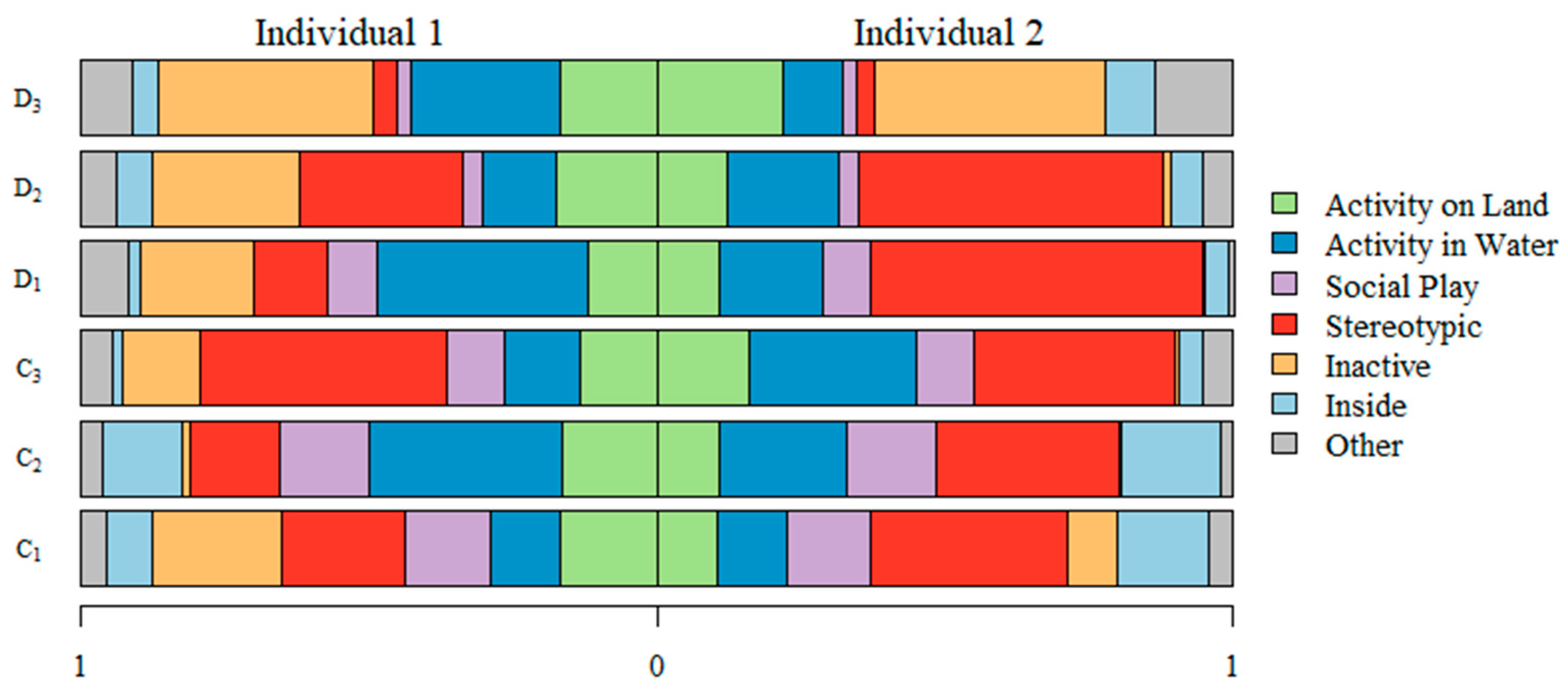
3.1. Proportion of Time Each Individual Spent on Each Behavior

The time spent on different behaviors varied between all the observation sessions and the individuals. Figure 1 shows that individual 2 generally spent a greater amount of time on the behavior ‘stereotypic’ and a smaller amount of time on ‘inactive’ behavior compared to individual 1. However, the amount of time the two individuals spent on these behaviors varied greatly between observation sessions. When comparing the two individuals’ ‘stereotypic’ and ‘inactive’ behavior for treatment D, a significant difference, between the two individuals, was observed for both behaviors. For this treatment, individual 1 spent a greater amount of time being ‘inactive’ than individual 2 (p < 0.05). The opposite was found for the amount of time the individuals spent on ‘stereotypic’ behavior, meaning that individual 2 spent more time on ‘stereotypic’ behavior than individual 1 (p < 0.01) (see Appendix B). Furthermore, it was found that individual 1 spent significantly more time being ‘inactive’ for treatment D in comparison to treatment C (p < 0.05) (see Appendix B).

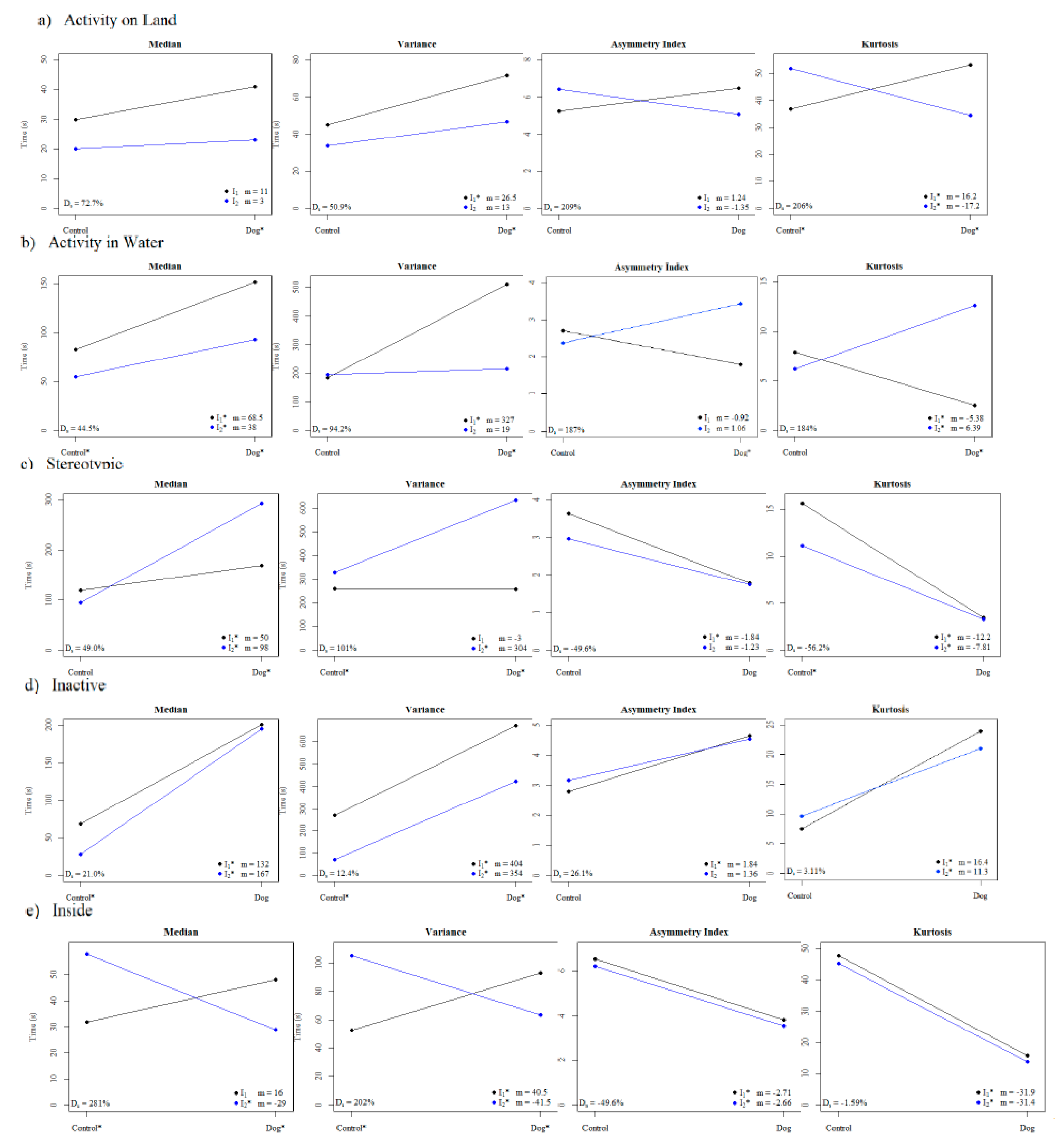
3.2. Reaction Norms for Testing Differences between Individuals and Treatments

An increase in the median time spent on each behavior between treatment C and D could be observed for both individuals and all behaviors, except the median time individual 2 spent ‘inside’, which showed a decrease between treatment C and D (p < 0.01) (Figure 2) (see Appendix D). For the three behaviors of ‘activity in water’, ‘stereotypic’ and ‘inactive’, significant differences in the median time were found between the two treatments for each individual (p < 0.01) (see Appendix D). When comparing the median time spent on ‘stereotypic’ behavior, a significant difference was found between the individuals for treatment D (p < 0.001) but not for treatment C (see Appendix D). For the behavior ‘inactive’, a significant difference was observed between the individuals for treatment C (p < 0.001). For most behaviors, it was found, for both individuals, that the variances increased between treatment C and D (Figure 2) (see Appendix D). The opposite was found for the behavior stereotypic’ of individual 1 and the behavior ‘inside’ for individual 2 (p < 0.01), meaning that the variances decreased between treatment C and D for these combinations (see Appendix D). For the behaviors ‘inactive’ and ‘inside’, significant differences were found between the variances of both individuals (p < 0.05) and between those of the two treatments (p < 0.01) (see Appendix D). There were also significant differences found between the variances of time spent on ‘stereotypic’ behavior between the two individuals for both treatments (p < 0.01) and between the two treatments for individual 2 (p < 0.001) (see Appendix D).
When comparing the asymmetry indices of the two treatments, results varied greatly for both individuals in terms of the asymmetry index between the two treatments (Figure 2) (see Appendix D). Significant differences between the asymmetry indices of the two treatments were found for the behaviors ‘stereotypic’, ‘inactive’ and ‘inside’ of individual 1 (p < 0.05), whereas for individual 2 it was only the behavior ‘inside’ that showed a significant difference (p < 0.01). A significant difference between the individuals for treatment D for ‘activity in water’ was also found, where individual 2 had a significant higher asymmetry index than individual 1 (p < 0.05). Furthermore, no significant differences were found between the two individuals for either of the two treatments (see Appendix D).
Similar to the asymmetry indices, great variation in whether the slope was positive or negative when comparing the kurtoses of the two treatments was also found for the different behaviors (Figure 2) (see Appendix D). For all behaviors, significant differences were found between the kurtoses of the two treatments for both individuals (p < 0.001). When comparing the kurtoses of the two individuals for treatment C, significant differences were found for the behaviors ‘activity on land’ and ‘stereotypic’ (p < 0.01) (see Appendix D). For treatment D, significant differences were found between the kurtoses of the two individuals for the behaviors ‘activity on land’ and ‘activity in water’ (p < 0.001) (see Appendix D).
The randomized moving average of the medians show that the medians of each behavior stabilize within the three observation sessions for both individuals and both treatments. The same was found for the randomized moving average of the variances (see Appendix E).

4. Discussion

4.1. Results of the Case Study

The results of the case study demonstrate the value of behavioral instability as a new quantitative method of behavior assessment. In this case study, an increase in median time and variance was found for most behaviors when the individuals were exposed to the olfactory stimuli of dog odor. This indicates that the occurrences of a behavior generally lasted longer when the individuals were provided with the olfactory stimuli, but also that the individuals were less predictable during the time they were engaged in each occurrence of a behavior. The effect of stimuli on the asymmetry index and kurtosis varied greatly between the individuals and behaviors. This demonstrates that there was a variation in predictability for the behaviors of both individuals when exposed to the olfactory stimuli.
The difference found in the two individuals’ responses to olfactory stimuli is a good example of how individuals can respond differently to environmental stress. This exhibits how the understanding of different behavioral reaction norms is important in the evaluation of welfare in captive animals [7,26], implying that different individuals can benefit from different types of enrichment in order to increase their welfare. When exposed to olfactory stimuli, there was a significant difference between the two individuals in the amount of time each spent on ‘stereotypic’ and ‘inactive’ behavior (Appendix B). One individual spent less time being ‘stereotypic’ and more time on ‘inactive’ behavior, while the other individual spent less time being ‘inactive’ and more time on ‘stereotypic’ behavior (Figure 1). The same was found when comparing the quantitative variables—median, variance, asymmetry index and kurtosis—of the data for the two individuals. This analysis showed significant differences in medians for treatment D and variances for treatment C and treatment D of time spent on ‘stereotypic’ behavior between the individuals. These differences were larger when the individuals were exposed to olfactory stimuli (Figure 2). This demonstrates that the individuals responded differently to the stimulus, supporting the statement that individuals with different behavioral reaction norms react differently to the same stimulus, as they often have different ways of coping with changes in their environment [9]. When comparing the asymmetry indices of both individuals for ‘stereotypic’ and ‘inactive’ behavior it was found that there was a smaller difference between the individuals, when exposed to stimuli, than under normal conditions; this means that the distributions were more similar. These various results indicate the importance of using different quantitative variables.

4.2. Reliability of Results

Despite the fact that this investigation has been conducted within a relatively short period of time, the number of seconds in which the two individuals were observed (194,400 seconds per individual) is large compared to other previous studies where the instantaneous sampling technique has been utilized; see for example [1] with six individuals and with 19,200 seconds of observation per individual; [10] with 55 individuals and 17,472 seconds of observation per individual; [12] with two individuals and 19,200 seconds of observation per individual. There is only one study where the number of seconds of observation was higher than in our investigation; [11] with 10,965,600 seconds of observation but conducted on a single individual and over a long period.
Furthermore, the randomized moving average of medians and variances also show that the medians and variances of each behavior stabilize within the three observation sessions of each treatment (Appendix E). Therefore, we believe that we have provided a robust preliminary dataset where the genetic and environmental bias are minimized, as the two individuals were sisters and the period of investigation is very short, therefore less prone to environmental fluctuations. All these factors allow us to draw robust conclusions. At the same time, we have provided a solid theoretical framework which can be applied to behavioral studies in the immediate future.

4.3. Considerations when Removing Outliers

The results discussed were generally observed for all three data sets, but some slight differences were found due to the removal of outliers. When using the MAD method, only large values were indicated as outliers and removed due to the distribution of the data, whereas when using the IQR to identify outliers, an equal amount of values smaller and greater than the median were removed. When removing outliers using IQR, only the most frequent results are shown; it can be argued that this gives a better representation of the data. A similar argument presents itself when removing outliers using MAD, as this method removes extreme values that have a small likelihood of occurring. When studying behavior, the distribution of the data is usually skewed to the right; hence, the removal of outliers using MAD can remove important information, as an individual performing a behavior for a long time is also a part of their behavior and cannot simply be ignored [27]. Even though removing outliers presents some disadvantages, it can also be a resourceful tool when comparing individuals and treatments, since the removal of outliers can increase the amount of significant results. However, the original data set should always be analyzed as well. Ideally, behavioral data should be analyzed both with and without outliers, as the different methods supplement each other.

4.4. Applying Behavioral Instability to Behavioral Investigations

In this study, it is shown how behavioral instability can be applied to behavioral observations by investigating the median, variance, asymmetry indices and kurtosis of different behaviors. The results of this study supports that behavioral instability can be applied to a more traditional type of behavioral data, in which an ethogram and observations of different behaviors are used. Thus, behavioral instability can be introduced as a new quantitative method for analyzing traditional ethograms. This study used this new method along with the traditional methods, enabling a comparison of the two methods. One of the major issues when using the traditional methods for studying behavior is the lack of comparable systematic and quantitative results [13,16]. Traditional methods are primarily used to estimate the percentage of time spent on various activities [17]. This estimate is highly dependent on the ethogram used, as the percentage of time spent on one activity is always dependent on the amount of time spent on other activities. Comparisons between studies are, therefore, only possible if highly similar ethograms are used, which can prove difficult in the comparison of behavior between species. The application of the concept behavioral instability enables the comparison of behavior regardless of differences in ethograms. This is possible due to the method’s quantitative approach that uses the median, variance, asymmetry index and kurtosis. The advantage of this approach is that these variables for one behavior are less dependent on the other behaviors.
The traditional methods also lack a protocol ensuring systematic data sampling. The results of this study indicate the need for longer observation sessions, as short observation sessions lead to a higher risk of type II errors. However, if the data are symmetric-leptokurtic, the risk of type II errors is lower, thus making it possible to create a behavioral analysis based on short observation sessions. When applying the concept of behavioral instability to behavioral studies, the data should be sampled using continuous focal sampling over the entire day since the occurrence of different behaviors has been observed to change throughout the day. The results of this study showed that many behaviors occurred for both shorter and longer periods of time and, therefore, information can be lost when using sampling techniques such as instantaneous sampling. Altmann [17] states that instantaneous sampling is primarily used for studying the proportion of time spent on various activities. However, the results would not be accurate, as behaviors shorter than the time between two preselected sampling instances would most likely not be recorded. When using this new quantitative method of applying behavioral instability, it is, therefore, important that sampling is conducted throughout the entire day using continuous focal sampling.
While the quantitative results of this new method enable comparisons between studies, traditional methods should not be dismissed, as valuable information also lies in knowing when an individual performs various behaviors throughout the day and the proportion of the day spent on different behaviors. It is suggested that the two methods are used collaboratively, comparing and combining the results of both approaches, in order to obtain the most reliable results. The application of the concept behavioral instability to traditional behavioral analyses allows quantitative data collection. This can provide researchers with a relatively unbiased evaluation of behavioral responses and the effectiveness of enrichment manipulation, which can contribute to the improvement of enrichment programs and animal welfare in captivity [13]. It has been debated whether the study of behavioral reaction norms can provide new insights for the field of behavioral ecology [7]. The use of behavioral instability as a new quantitative and systematic method for studying behavioral responses could be highly relevant when studying animal conservation. When captive populations are being managed with the aim of re-introducing individuals to the wild, an understanding of the behavioral reaction norms can provide insight on how to conserve behavioral responses that could be beneficial in the wild.

Author Contributions

All authors have contributed equally and have conceptualized the project and done the methodology. C.P. and T.H.J. provided the resources, while A.C.L., A.G., H.L. and M.G.L. did the investigation and data curation. A.C.L., A.G. and H.L. did the formal analysis and visualization and took the lead in writing the manuscript. All authors provided critical feedback and helped shape the research, analysis and manuscript. C.P. and T.H.J. were responsible for the project. All authors have read and agreed to the published version of the manuscript.

Funding

This investigation was supported by the Aalborg Zoo Conservation Foundation (Grant Number: 3-2018).

Acknowledgments

The authors wish to thank the staff of Aalborg Zoo, with special thanks to Katrine Christensen and Frank Thomsen for their time and involvement in this study. We also thank three anonymous reviewers and Rabby Zhang for invaluable suggestions and help.

Conflicts of Interest

The authors declare no conflict of interest.

Appendix A

Map of the polar bear enclosure at Aalborg Zoo. Only one exhibit was used in the study, this exhibit is indicated on the map. The other exhibit housed the mother of the two polar bears studied. The placement of the four cameras used for surveillance is shown.
Symmetry 12 00603 i001

Appendix B

χ2 Test of Total Time

χ2 test results for testing the percentages of time spent on each behavior for the entire observation session based on pooled data for treatment C and treatment D of each individual. A blank space indicates that the behavior consisted of less than 5% of the observation session. Results when comparing individual 1 with individual 2 are shown on the left and results comparing treatment C and D are shown on the right.
Behaviorχ2 Test Comparing Individualsχ2 Test Comparing Treatments
C p o o l e d D p o o l e d I 1 p o o l e d I 2 p o o l e d
Activity on landχ2 = 0.3542χ2 = 6.730 × 10⁻³χ2 = 1.388 × 10⁻⁴χ2 = 0.2510
p = 0.5518 p = 0.9346 p = 0.9906 p = 0.6164
Activity in waterχ2 = 0.05417χ2 = 2.058χ2 = 0.6791χ2 = 0.7223
p = 0.8160 p = 0.1514 p = 0.4099 p = 0.3954
Social playχ2 = 2.666 × 10⁻⁴
p = 0.9870
Stereotypicχ2 = 0.8345χ2 = 9.695χ2 = 3.104χ2 = 0.2462
p = 0.3610 p = 0.001848 p = 0.07808 p = 0.6197
Inactive χ2 = 4.501χ2 = 5.736
p = 0.03388 p = 0.01661
Insideχ2 = 1.118 χ2 = 2.169
p = 0.2904 p = 0.1408

Appendix C

Appendix C.1. Slopes of Medians, Variances, Asymmetry Indices and Kurtoses

For each individual the median time and variance of time spent on a given behavior are shown for treatment C and for treatment D along with trend lines between the medians and the variances for the two individuals. The asymmetry index and kurtosis are also shown for treatment C and for treatment D and each individual along with trend lines between the asymmetry indices and kurtoses of the two treatments for the same individual. The medians, variances, asymmetry indices and kurtoses are based in pooled data. The slope (m) and difference in slope in percent (Ds) are given for each comparison. The medians, variances, asymmetry indices and kurtoses were compared by χ2 test with Yates correction. Comparisons in which the χ2 test resulted in significant results between the two individuals for the same treatment are indicated by * next to the relative treatment. Comparisons in which the χ2 test resulted in significant results between the two treatments for the same individual are indicated by * next to the relative individual. The medians are not shown for the dataset where outliers were removed outside IQR since the values are identical to the values shown in figures for the data set with all data points.

Appendix C.2. Dataset where Outliers were Removed outside IQR

Activity on land
Symmetry 12 00603 i002
Activity in water
Symmetry 12 00603 i003
Stereotypic
Symmetry 12 00603 i004
Inactive
Symmetry 12 00603 i005
Inside
Symmetry 12 00603 i006

Appendix C.3. Dataset where Outliers were Removed Using the MAD Method

Activity on land
Symmetry 12 00603 i007
Activity in water
Symmetry 12 00603 i008
Stereotypic
Symmetry 12 00603 i009
Inactive
Symmetry 12 00603 i010
Inside
Symmetry 12 00603 i011

Appendix D

χ2 Test for Distribution of Statistics

χ2 test results for comparing the medians, variances, asymmetry indices and kurtoses of the pooled data for each behavior for the different data sets. The pooled data for asymmetry indices and kurtoses were multiplied by 10 before the perpetration of the χ2 test. Results when comparing individual 1 and individual 2 are shown on the left and results comparing treatment C and D are shown on the right. Comparisons for which χ2 test could not be performed due to negative values are indicated by -. χ2 tests for medians for the data set where outliers were removed outside IQR are not shown since the medians are the same as for the dataset containing all data points.
D.1.a: χ2 Tes t of medians, all data points
Behaviorχ2 Test Comparing Individualsχ2 Test Comparing Treatments
C p o o l e d D p o o l e d I 1 p o o l e d I 2 p o o l e d
Activity on landχ2 = 2.000χ2 = 5.063χ2 = 1.704χ2 = 0.2093
p = 0.1573p = 0.02445p = 0.1917p = 0.6473
Activity in waterχ2 = 5.681χ2 = 14.00χ2 = 20.01χ2 = 9.757
p = 0.01715p = 0.0001831p = 7.705 × 10⁻⁶p = 0.001787
Stereotypicχ2 = 2.692χ2 = 33.28χ2 = 8.681χ2 = 101.0
p = 0.1009p = 7.974 × 10⁻⁹p = 0.003216p < 2.2 × 10⁻¹⁶
Inactiveχ2 = 17.33χ2 = 0.090909χ2 = 64.53χ2 = 125.1
p = 3.142 × 10⁻⁵p = 0.7630p = 9.491 × 10⁻¹⁶p < 2.2 × 10⁻¹⁶
Insideχ2 = 7.511χ2 = 4.6883χ2 = 3.200χ2 = 9.667
p = 0.006130p = 0.03037p = 0.07364p = 0.001876
D.1.b: χ2 test of variances, all data points
Behaviorχ2 Test Comparing Individualsχ2 Test Comparing Treatments
CpooledDpooled I 1 p o o l e d I 2 p o o l e d
Activity on landχ2 = 1.607χ2 = 5.1802χ2 = 6.0279χ2 = 2.0994
p = 0.2049p = 0.02285p = 0.01408p = 0.1474
Activity in waterχ2 = 0.3485χ2 = 120.68χ2 = 153.85χ2 = 0.92631
p = 0.5550p < 2.2 × 10⁻¹⁶p < 2.2 × 10⁻¹⁶p = 0.3358
Stereotypicχ2 = 8.000χ2 = 160.06χ2 = 0.02381χ2 = 96.901
p = 0.004677p < 2.2 × 10⁻¹⁶p = 0.8774p < 2.2 × 10⁻¹⁶
Inactiveχ2 = 117.65χ2 = 56.668χ2 = 172.9χ2 = 254.14
p < 2.2 × 10⁻¹⁶p = 5.15910−14p < 2.2 × 10⁻¹⁶p < 2.2 × 10⁻¹⁶
Insideχ2 = 17.5χ2 = 5.5607χ2 = 11.273χ2 = 10.221
p = 2.873 × 10⁻⁵p = 0.01837p = 0.0007863p = 0.001388
D.1.c: χ2 test of asymmetry indices, all data points
Behaviorχ2 Test Comparing Individualsχ2 Test Comparing Treatments
CpooledDpooled I 1 p o o l e d I 2 p o o l e d
Activity on landχ2 = 1.201χ2 = 1.713χ2 = 1.311χ2 = 1.588
p = 0.2731p = 0.1905p = 0.2523p = 0.2076
Activity in waterχ2 = 0.2064χ2 = 5.254χ2 = 1.886χ2 = 1.934
p = 0.6496p = 0.0219p = 0.1697p = 0.1644
Stereotypicχ2 = 0.6759χ2 = 0.007748χ2 = 6.280χ2 = 3.216
p = 0.411p = 0.9299p = 0.01221p = 0.07293
Inactiveχ2 = 0.2501χ2 = 0.01137χ2 = 4.58χ2 = 2.384
p = 0.617p = 0.9151p = 0.03235p = 0.1226
Insideχ2 = 0.07902χ2 = 0.09389χ2 = 7.104χ2 = 7.228
p = 0.7786p = 0.7593p = 0.007693p = 0.007178
D.1.d: χ2 test of kurtoses, all data points
Behaviorχ2 Test Comparing Individualsχ2 Test Comparing Treatments
CpooledDpooled I 1 p o o l e d I 2 p o o l e d
Activity on landχ2 = 25.15χ2 = 39.02χ2 = 29.34χ2 = 34.19
p = 5.305 × 10⁻⁷p = 4.187 × 10⁻¹⁰p = 6.09 × 10⁻⁸p = 4.996 × 10⁻⁹
Activity in waterχ2 = 2.062χ2 = 66.84χ2 = 27.65χ2 = 21.70
p = 0.1511p = 2.945e-16p = 1.452 × 10⁻⁷p = 3.196 × 10⁻⁶
Stereotypicχ2 = 7.574χ2 = 0.02510χ2 = 77.88χ2 = 42.31
p = 0.005922p = 0.8741p < 2.2 × 10⁻¹⁶p = 7.788 × 10⁻¹¹
Inactiveχ2 = 2.824χ2 = 1.915χ2 = 86.12χ2 = 41.71
p = 0.09284p = 0.1664p < 2.2 × 10⁻¹⁶p = 1.059 × 10⁻¹⁰
Insideχ2 = 0.6862χ2 = 1.432χ2 = 159.7χ2 = 167.1
p = 0.4075p = 0.2315p < 2.2 × 10⁻¹⁶p < 2.2 × 10⁻¹⁶
D.2.b: χ2 test of variances, IQR
Behaviorχ2 Test Comparing Individualsχ2 Test Comparing Treatments
C p o o l e d D p o o l e d I 1 p o o l e d I 2 p o o l e d
Activity on landχ2 = 1.581χ2 = 5.400χ2 = 5.924χ2 = 1.882
p = 0.2086p = 0.02014p = 0.01486p = 0.1701
Activity in waterχ2 = 0.5436χ2 = 22.42χ2 = 41.12χ2 = 6.208
p = 0.4609p = 2.194 × 10⁻⁶p = 1.429 × 10⁻¹⁰p = 0.0127
Stereotypicχ2 = 0.6429χ2 = 130.9χ2 = 1.766χ2 = 141.3
p = 0.4227p < 2.2 × 10⁻¹⁶p = 0.1839p < 2.2 × 10⁻¹⁶
Inactiveχ2 = 36.92χ2 = 1.313χ2 = 48.00χ2 = 124.5
p = 1.234 × 10⁻⁹p = 0.2519p = 4.255 × 10⁻¹²p < 2.2 × 10⁻¹⁶
Insideχ2 = 11.77χ2 = 15.99χ2 = 20.56χ2 = 8.25
p = 0.0006032p = 6.351 × 10⁻⁵p = 5.771 × 10⁻⁶p = 0.004075
D.2.c: χ2 test of asymmetry indices, IQR
Behaviorχ2 Test Comparing Individualsχ2 Test Comparing Treatments
C p o o l e d D p o o l e d I 1 p o o l e d I 2 p o o l e d
Activity on landχ2 = 0.9885χ2 = 1.231χ2 = 0.1648χ2 = 0.0821
p = 0.3201p = 0.2673p = 0.6848p = 0.7745
Activity in waterχ2 = 0.07778χ2 = 1.211χ2 = 0.1620χ2 = 0.9592
p = 0.7803p = 0.2711p = 0.6873p = 0.3274
Stereotypicχ2 = 0.518χ2 = 1.044χ2 = 0.3828χ2 = 5.069
p = 0.4715p = 0.3069p = 0.5361p = 0.02436
Inactiveχ2 = 0.0781χ2 = 2.675χ2 = 0.2099χ2 = 0.8363
p = 0.7799p = 0.1019p = 0.6468p = 0.3605
Insideχ2 = 4.791χ2 = 0.04612χ2 = 2.024χ2 = 0.3942
p = 0.02861p = 0.8300p = 0.1548p = 0.5300
D.2.d: χ2 test of kurtoses, IQR
Behaviorχ2 Test Comparing Individualsχ2 Test Comparing Treatments
C p o o l e d D p o o l e d I 1 p o o l e d I 2 p o o l e d
Activity on land--- -
Activity in water----
Stereotypic----
Inactiveχ2 = 4.858χ2 = 34.39χ2 = 3.096χ2 = 8.407
p = 0.02752p = 4.518 × 10⁻⁹p = 0.07851p = 0.003738
Inside----
D.3.a: χ2 test of medians, MAD
Behaviorχ2 Test Comparing Individualsχ2 Test Comparing Treatments
C p o o l e d D p o o l e d I 1 p o o l e d I 2 p o o l e d
Activity on landχ2 = 2.814χ2 = 5.333χ2 = 0.4237χ2 = 0
p = 0.09345p = 0.02092p = 0.5151p = 1
Activity in waterχ2 = 2.919χ2 = 1.651χ2 = 3.6552χ2 = 5.434
p = 0.08753p = 0.1988p = 0.05589p = 0.01975
Stereotypicχ2 = 11.21χ2 = 46.41χ2 = 3.435χ2 = 131.1
p = 0.0008153p = 9.609 × 10⁻¹²p = 0.06385p < 2.2 × 10⁻¹⁶
Inactiveχ2 = 9.1351χ2 = 15.125χ2 = 23.11χ2 = 116.5
p = 0.0002507p = 0.0001469p = 1.528 × 10⁻⁶p < 2.2 × 10⁻¹⁶
Insideχ2 = 2.522χ2 = 0.8649χ2 = 2.882χ2 = 0.6712
p = 0.1122p = 0.3524p = 0.08956p = 0.4126
D.3.b: χ2 test of variances, MAD
Behaviorχ2 Test Comparing Individualsχ2 Test Comparing Treatments
C p o o l e d D p o o l e d I 1 p o o l e d I 2 p o o l e d
Activity on landχ2 = 4.373χ2 = 9.727χ2 = 4.580χ2 = 1.142
p = 0.03873p = 0.001816p = 0.03234p = 0.2853
Activity in waterχ2 = 6.0945χ2 = 11.48χ2 = 19.16χ2 = 11.99
p = 0.01356p = 0.000704p = 1.203 × 10⁻⁵p = 0.000536
Stereotypicχ2 = 3.647χ2 = 152.4χ2 = 4.179χ2 = 247.5
p = 0.05616p < 2.2 × 10⁻¹⁶p = 0.04093p < 2.2 × 10⁻¹⁶
Inactiveχ2 = 22.38χ2 = 59.73χ2 = 51.22χ2 = 298.2
p = 2.36 × 10⁻⁶p = 1.091 × 10⁻¹⁴p = 8.25 × 10⁻¹³p < 2.2 × 10⁻¹⁶
Insideχ2 = 21.59χ2 = 9.940χ2 = 24.30χ2 = 8.127
p = 3.383 × 10⁻⁶p = 0.001618p = 8.229 × 10⁻⁷p = 0.00436
D.3.c: χ2 test of asymmetry indices, MAD
Behaviorχ2 Test Comparing Individualsχ2 Test Comparing Treatments
C p o o l e d D p o o l e d I 1 p o o l e d I 2 p o o l e d
Activity on landχ2 = 0.1273χ2 = 0.01984χ2 = 0.1χ2 = 0.01004
p = 0.7212p = 0.888p = 0.7518p = 0.9202
Activity in waterχ2 = 0.03937χ2 = 0.3240χ2 = 0.003371χ2 = 0.09825
p = 0.8427p = 0.5692p = 0.9537p = 0.7539
Stereotypicχ2 = 0.09412χ2 = 0.02645χ2 = 0.003557χ2 = 0.2793
p = 0.759p = 0.8708p = 0.9524p = 0.5972
Inactiveχ2 = 0.4181χ2 = 1.288χ2 = 0.2054χ2 = 0.001563
p = 0.5179p = 0.2564p = 0.6504p = 0.9685
Insideχ2 = 0.0004049χ2 = 0.2091χ2 = 0.03389χ2 = 0.08620
p = 0.9839p = 0.6475p = 0.8539p = 0.7691
D.3.d: χ2 test of kurtoses, MAD
Behaviorχ2 Test Comparing Individualsχ2 Test Comparing Treatments
C p o o l e d D p o o l e d I 1 p o o l e d I 2 p o o l e d
Activity on landχ2 = 31.44χ2 = 0χ2 = 31.44χ2 = 0
p = 2.055 × 10⁻⁸p = 1p = 2.055 × 10⁻⁸p = 1
Activity in waterχ2 = 71.67χ2 = 31.14χ2 = 5.4724χ2 = 1.140
p < 2.2 × 10⁻¹⁶p = 2.391 × 10⁻⁸p = 0.01932p = 0.2858
Stereotypicχ2 = 11.406χ2 = 1.034χ2 = 1.199χ2 = 29.12
p = 0.0007321p = 0.3092p = 0.2736p = 6.79 × 10⁻⁸
Inactiveχ2 = 108.5χ2 = 166.4χ2 = 31.51χ2 = 9.219
p < 2.2 × 10⁻¹⁶p < 2.2 × 10⁻¹⁶p = 1.981 × 10⁻⁸p = 0.002395
Insideχ2 = 0χ2 = 81χ2 = 16.12χ2 = 28.47
p = 1p < 2.2 × 10⁻¹⁶p = 5.932 × 10⁻⁵p = 9.513 × 10⁻⁸
Moving medians and variances
Plots showing the moving medians and variances of all the data points for each behavior. The moving medians and variances were calculated based on the pooled data for treatment C (blue) and treatment D (orange). The pooled data were randomized prior to calculating the moving medians and variances.

Appendix E

Appendix E.1. Moving Medians

Activity on land
Symmetry 12 00603 i012
Activity in water
Symmetry 12 00603 i013
Stereotypic
Symmetry 12 00603 i014
Social Play
Symmetry 12 00603 i015
Inactive
Symmetry 12 00603 i016
Inside
Symmetry 12 00603 i017

Appendix E.2. Moving Variances

Activity on land
Symmetry 12 00603 i018
Activity in water
Symmetry 12 00603 i019
Stereotypic
Symmetry 12 00603 i020
Social Play
Symmetry 12 00603 i021
Inactive
Symmetry 12 00603 i022
Inside
Symmetry 12 00603 i023

References

  1. Myers, P.; Young, J. Consistent individual behavior: Evidence of personality in black bears. J. Ethol. 2018, 36, 117–124. [Google Scholar] [CrossRef] [Green Version]
  2. Santicchia, F.; Wauters, L.A.; Dantzer, B.; Westrick, S.E.; Ferrari, N.; Romeo, C.; Palme, R.; Preatoni, D.G.; Martinoli, A. Relationships between personality traits and the physiological stress response in a wild mammal. Curr. Zool. 2019, 66, 197–204. [Google Scholar] [CrossRef]
  3. Thys, B.; Lambreghts, Y.; Pinxten, R.; Eens, M. Nest defence behavioral reaction norms: Testing life-history and parental investment theory predictions. R. Soc. Open Sci. 2019, 6, 182180. [Google Scholar] [CrossRef] [PubMed] [Green Version]
  4. Montiglio, P.-O.; Garant, D.; Pelletier, F.; Re´ale, D. Personality differences are related to long-term stress reactivity in a population of wild eastern chipmunks, Tamias striatus. Anim. Behav. 2012, 84, 1071–1079. [Google Scholar] [CrossRef]
  5. Luo, L.; Reimert, I.; de Haas, E.N.; Kemp, B.; Bolhuis, J.E. Effects of early and later life environmental enrichment and personality on attention bias in pigs (Sus scrofa domesticus). Anim. Cogn. 2019, 22, 959–972. [Google Scholar] [CrossRef] [Green Version]
  6. Dingemanse, N.J.; Kazem, A.J.N.; Réale, D.; Wright, J. Behavioural reaction norms: Animal personality meets individual plasticity. Trends Ecol. Evol. 2009, 25, 82–89. [Google Scholar] [CrossRef]
  7. Wilson, V.; Guenther, A.; Øverli, Ø.; Seltmann, M.W.; Altschul, D. Future directions for personality research: Contributing new insights to the understanding of animal behavior. Animals 2019, 9, 240. [Google Scholar] [CrossRef] [Green Version]
  8. Clubb, R.; Mason, G.J. Animal welfare: Captivity effects on wide-ranging carnivores. Nature 2003, 425, 473–474. [Google Scholar] [CrossRef]
  9. Mason, G.J.; Latham, N.R. Can’t stop, Won’t stop: Is stereotypy a reliable animal welfare indicator? Anim. Welf. 2004, 13, 57–69. [Google Scholar]
  10. Shepherdson, D.; Lewis, K.D.; Carlstead, K.; Bauman, J.; Perrin, N. Individual and environmental factors associated with stereotypic behavior and fecal glucocorticoid metabolite levels in zoo housed polar bears. Appl. Anim. Behav. Sci. 2013, 147, 268–277. [Google Scholar] [CrossRef]
  11. Carlstead, K.; Seidensticker, J. Seasonal variation in stereotypic pacing in an american black bear Ursus americanus. Behav. Process. 1991, 25, 155–161. [Google Scholar] [CrossRef]
  12. Ross, S.R. Issues of choice and control in the behaviour of a pair of captive polar bears Ursus maritimus. Behav. Process. 2006, 73, 117–120. [Google Scholar] [CrossRef] [PubMed]
  13. Shyne, A. Meta-analytic review of the effects of enrichment on stereotypic behavior in zoo mammals. Zoo Biol. 2006, 25, 317–337. [Google Scholar] [CrossRef]
  14. Cless, I.T.; Voss-Hoynes, H.A.; Ritzmann, R.E.; Lukas, K.E. Defining pacing quantitatively: A comparison of gait characteristics between pacing and non-repetitive locomotion in zoo-housed polar bears. Appl. Anim. Behav. Sci. 2015, 169, 78–85. [Google Scholar] [CrossRef]
  15. Carlstead, K.; Seidensticker, J.; Baldwin, R. Environmental enrichment for zoo bears. Zoo Biol. 1991, 10, 3–16. [Google Scholar] [CrossRef]
  16. Rose, P.E.; Nash, S.M.; Riley, L.M. To pace or not to pace? A Review of what abnormal repetitive behavior tells us about zoo animal management. J. Vet. Behav. 2017, 20, 11–21. [Google Scholar] [CrossRef]
  17. Altmann, J. Observational study of behavior: Sampling methods. Behaviour 1974, 49, 227–267. [Google Scholar] [CrossRef] [Green Version]
  18. Bashaw, M.J.; Kelling, A.S.; Bloomsmith, M.A.; Maple, T.L. Environmental effects on the behavior of zoo-housed lions and tigers, with a case study of the effects of a visual barrier on pacing. J. Appl. Anim. Welf. Sci. 2007, 10, 95–109. [Google Scholar] [CrossRef]
  19. Pertoldi, C.; Bahrndorff, S.; Novicic, Z.K.; Rohde, P.D. The novel concept of ”behavioral instability” and its potential applications. Symmetry 2016, 8, 135. [Google Scholar] [CrossRef] [Green Version]
  20. Bech-Hansen, M.; Kallehauge, R.M.; Bruhn, D.; Castenschiold, J.H.F.; Gehrlein, J.B.; Laubek, B.; Jensen, L.F.; Pertoldi, C. Effect of landscape elements on the symmetry and variance of the spatial distribution of individual birds within foraging flocks of geese. Symmetry 2019, 11, 1103. [Google Scholar] [CrossRef] [Green Version]
  21. Clark, F.; King, A.J. A critical review of zoo-based olfactory enrichment. In Chemical Signals in Vertebrates 11; Hurst, J.L., Beynon, R.J., Roberts, S.C., Wyatt, T.D., Eds.; Springer: New York, NY, USA, 2008. [Google Scholar]
  22. RStudio Team. RStudio: Integrated Development for R; RStudio, Inc.: Boston, MA, USA, 2016. [Google Scholar]
  23. Hammer, Ø.; Harper, D.A.T.; Ryan, P.D. Past: Paleontological statistics software package for education and data analysis. Palaeontol. Electron. 2001, 4, 1–9. [Google Scholar]
  24. Leys, C.; Ley, C.; Klein, O.; Bernard, P.; Licata, L. Detecting outliers: Do not use standard deviation around the mean, use absolute deviation around the median. J. Exp. Soc. Psychol. 2013, 49, 764–766. [Google Scholar] [CrossRef] [Green Version]
  25. Zar, J.H. Biostatistical Analysis, 4th ed.; Pearson: London, UK; Northern Illinois University: DeKalb, IL, USA, 1999. [Google Scholar]
  26. Yosef, R.; Raz, M.; Ben-Baruch, N.; Shmueli, L.; Kosicki, L.J.Z.; Fratczak, M.; Tryjanowski, P. Directional preferences of dogs’ changes in the presence of a bar magnet: Educational experiments in Israel. J. Vet. Behav. 2019, in press. [Google Scholar] [CrossRef]
  27. Rousseeuw, P.J.; Croux, C. Alternatives to the median absolute deviation. J. Am. Stat. Assoc. 1993, 88, 1273–1283. [Google Scholar] [CrossRef]
Figure 1. Proportion of time each individual spent on the different behaviors for each of the three observation sessions for each treatment (C = control, D = dog-scented object). The three lower bars represent the control observation sessions and the three upper bars represent the observation sessions in which the individuals were exposed to olfactory stimuli. The data were pooled and compared by χ2 tests with a Yates correction (see Appendix B).
Symmetry 12 00603 g001
Figure 2. Behavioral reaction norms; for each individual, the median and variance of time spent on a given behavior are shown for treatment C and for treatment D along with trend lines between the medians and between the variances of the two treatments for the same individual. The asymmetry index and kurtosis are also shown for treatment C and for treatment D and each individual along with trend lines between the asymmetry indices and between the kurtoses of the two treatments for the same individual. The medians, variances, asymmetry indices and kurtoses are based on pooled data. The slope (m) and difference in slope in percent (DS) are given for each comparison. The medians, variances, asymmetry indices and kurtoses were compared by χ2 tests with a Yates correction. Comparisons in which the χ2 test resulted in significant results between the two individuals for the same treatment are indicated by * next to the relative treatment. Comparisons in which the χ2 test resulted in significant results between the two treatments for the same individual are indicated by * next to the relative individual. For further details on χ2 values, see Appendix D.
Symmetry 12 00603 g002
Table 1. Behavioral ethogram.
BehaviorDescription
Activity on landLocomotion and interaction with objects while on land
Activity in waterLocomotion and interaction with objects while submerged in water
Social playIndividuals interacting playfully of fighting with each other, possibly while interacting with objects.
StereotypicRepeating a specific walking pattern or movement aimlessly
InactiveResting or sleeping; laying down or sitting with minimal movement
InsideInside the den and therefore out of sight
OtherEating, drinking, urinating, defecating, maintenance of coat (e.g., by rolling in gravel) and out of sight due to blind camera angles

