Nonstandard Action of Diffeomorphisms and Gravity’s Anti-Newtonian Limit

Department of Physics and Astronomy, University of Pittsburgh, 100 Allen Hall, Pittsburgh, PA 15260, USA
Symmetry 2020, 12(5), 752; https://0-doi-org.brum.beds.ac.uk/10.3390/sym12050752
Submission received: 30 March 2020
/
Revised: 9 April 2020
/
Accepted: 12 April 2020
/
Published: 6 May 2020
(This article belongs to the Special Issue Symmetry and Quantum Gravity)
Abstract
:A tensor calculus adapted to the Anti-Newtonian limit of Einstein gravity is developed. The limit is defined in terms of a global conformal rescaling of the spatial metric. This enhances spacelike distances compared to timelike ones and in the limit effectively squeezes the lightcones to lines. Conventional tensors admit an analogous Anti-Newtonian limit, which however transforms according to a non-standard realization of the spacetime Diffeomorphism group. In addition to the type of the tensor the transformation law depends on, a set of integer-valued weights is needed to ensure the existence of a nontrivial limit. Examples are limiting counterparts of the metric, Einstein, and Riemann tensors. An adapted purely temporal notion of parallel transport is presented. By introducing a generalized Ehresmann connection and an associated orthonormal frame compatible with an invertible Carroll metric, the weight-dependent transformation laws can be mapped into a universal one that can be read off from the index structure. Utilizing this ‘decoupling map’ and a realization of the generalized Ehresmann connection in terms of scalar field, the limiting gravity theory can be endowed with an intrinsic Levi–Civita type notion of spatio-temporal parallel transport.
1. Introduction
In a formulation where the geometry of a foliated manifold M is specified by a lapse-like field , a shift-like field , and a spatial metric with inverse , consider the following action
Here , with the d-dimensional Lie derivative, and is a minimally coupled scalar field made dimensionless by multiplying with the square root of the gravitational constant. Its potential is real valued and has a constant term taken out. The action (1) has a sound motivation as the Anti-Newtonian limit of Einstein gravity minimally coupled to a scalar field . In form the gravitational action S is a functional of the lapse N, shift , spatial metric with inverse , and the scalar . The essential part of the scale transformation is , for real . For large spacelike distances are relatively enhanced and the lightcones appear to be squeezed to almost lines, thereby implementing an Anti-Newtonian limit. Applied to the gravitational action S the Ricci scalar of the spatial metric and spatial gradient term of the scalar field drop out for , and one is left with (1) (where the subscript 0 refers to . A more detailed motivation for this limit and the associated Anti-Newtonian expansion is presented in Section 2.1. For short, we shall refer to the gravity theory described by (1) as Sgravity. Here ‘S’ is a mnemonic used alternatively for ‘scaling’ or ‘strong coupling’.
The subject of this article are the symmetries of the action (1) and the development of a tensor calculus adapted to them. Since the Einstein–Hilbert action is usually motivated as the unique ‘generally covariant’ action ‘second order’ in derivatives, one might expect (1) to be invariant at best under a subclass of diffeomorphisms. Remarkably, (1) is invariant under the full spacetime Diffeomorphism group , which acts however in a non-standard way on the fields [1]. One may think of this as a realization of the abstract Diffeomorphism group different from the familiar tensorial one. We write
and refer to ’s invariance as one with respect to the realization. For the concatenation of two diffeomorphisms , the realization meets the basic requirement when acting on . We shall not pursue topological aspects of the Diffeomorphism group or the concomitant functional analytical aspects needed to turn into a bona-fide representation. In fact, there are more pressing questions to be answered first.
One is that is grossly under-determined by knowing only its action on . The standard tensor calculus is designed such that the generalized pull-back and push-forward of a diffeomorphism are automorphisms of the tensor algebra that commute with contractions. In particular, the pseudo-Riemannian metric entering the Einstein–Hilbert action is of course a second rank tensor and the push-forward defines a left action on it, . In a formulation the metric is parameterized in terms of lapse N, shift , and spatial metric via . Here are local spacetime coordinates and are local coordinates; we allow both signatures throughout, . On the constituent fields the tensorial realization acts in a nonlinear and unfamiliar way, recorded here (for the first time, we believe) in Equation (A33). By construction, the form of the matter coupled Einstein–Hilbert action is invariant under acting on . Of course differs from for generic . Denoting the scale transformation by , one finds that
for all . After renaming the fields this produces the realization on . The additional in ’s asymptotics is crucial and the integer will be referred to as ’s weight. A natural extension of this procedure to generic type tensors U is to search for weighted limits of the scaled tensorial realization
Here U refers to the tuple , of U’s block components defined with respect to the frame set by the foliation; each component may have to be rescaled by some , , in order to obtain a finite nonzero limit. Each transformed block is a linear combination of the other blocks with coefficients that may depend nonlinearly on . Scaling limits of part of a direct sum metric are known in Differential Geometry as “adiabatic limits”. They have been used to study connections, curvatures, and the spectra of covariant Laplacians [2,3,4], but to the best of our knowledge have not been applied to Einstein gravity itself. Since the term “adiabatic limit” is already taken in physics, we shall refer to (4) alternatively as “Anti-Newtonian limit” or simply as “-scaling limit”. The resulting transformation law will for generic differ from and will be taken as the defining characteristic of an Stensor of type and weight tuple w.
A nontrivial example is the counterpart of the Einstein tensor in Sgravity. With from (1) we define
where indicates that the -dependent terms are omitted (which are attributed to an analogously defined energy–momentum tensor for Sgravity). Then turns out to be an Stensor in the above sense of type and weight . Concretely, this amounts to a specific transformation law which we note here in linearized form:
Suitably interpreted is the linearized version of , where the descriptors of the infinitesimal diffeomorphisms , have been traded for , . These still comprise unconstrained functions of . For the block components of the Einstein tensor proper, , the corresponding gauge transformations differ from (6). This marks on the linearized level the difference between the universal tensorial realization and the weight-dependent scaling realization .
The limit construction (3) successfully defines the nonstandard realization for tensors of all types. It is however not an autonomous formalism in that it is rooted in the tensorial realization . On a foliated pseudo-Riemannian manifold one will naturally require the limits to be compatible with moving indices with the spacetime metric . This turns out to restrict the allowed weights and also allows one to define and to compute the transformation law autonomously, using the realization only.
An elegant way to code the same information is via decoupling map: for a given weight there are polynomial redefinitions of the Stensor’s blocks that transform multilinearly among themselves. For example in (6) the redefined blocks transform without the mixing terms in the middle equation. Generally, the redefined blocks satisfy decoupled transformation laws that can be read off from the index structure alone. The non-universal, weight-dependent aspects are coded by the redefinition, i.e., by the decoupling map.
The key ingredient in this construction is an auxiliary structure , transforming under generic diffeomorphisms as follows
For this is the transformation law of an Ehresmann connection. In fact, is an admissible gauge [1] in which the covariance group reduces to the group , , dubbed Carroll diffeomorphisms [5,6]. The generalized Ehresmann connection (7) allows one to maintain covariance under the full Diffeomorphism group. In terms of and one can introduce an orthonormal frame, which we call the SDiff frame,
It transforms without mixing under all of : , , while , are linear combinations of , respectively. The SDiff frame has several other noteworthy properties. First, it is metric compatible with respect to the following invertible, -dependent metric
That is, and hold. The more familiar degenerate Carroll metric [5,6,7,8] is given by , with pseudo-inverse . Second, the nonstandard action on induces a standard tensorial transformation for the and coordinate components of the frame (8). As a consequence the same holds for the ; mathematically they intertwine the with the realization of . Third, note that the spatial block of and the temporal part of are -independent. The non-mixing transformation laws of the SDiff frame (8) thereby entail
The spatial block of the metric and the temporal part of the contra-metric are separately fully diffeomorphism invariant! This can be seen as the characteristic feature of the Sgravity geometry compatible with the invariance of (1). These three properties conspire constructively to allow for the above decoupling maps. Utilizing them a fully covariant SCarroll–Levi–Civita connection can be defined, generalizing the one in [9]. Since can be realized in terms of a scalar as , Sgravity coupled to a scalar with can be endowed with an intrinsic Levi–Civita type notion of spatio-temporal parallel transport.
The article is organized as follows. In Section 2 we motivate the Sgravity action (1) in more detail and derive the transformation law (3) that ensures its invariance. In Section 3 we introduce the generalized Ehresmann connection (7) and discuss its ramifications: the existence of the SDiff frame (8) compatible with the invertible Carroll metric (9), whose coordinate components intertwine the with the realization. In Section 4.1 the limit construction (4) of Stensors is elucidated. Examples of Stensors and their linearized transformation laws are presented in Section 4.2. Section 4.3 constructs the decoupling maps. Different notations of covariant parallel transport are discussed in Section 5. Brief conclusions and an outlook are offered in Section 6. Appendix A revisits the tensor calculus of (pseudo-)Riemannian geometry with a focus on (occasionally new) results needed in the bulk of the paper.
2. Sgravity and Its Diffeomorphism Invariance
Written in form one can separate the kinematical from the dynamical spatial gradients in Einstein gravity. Then Sgravity describes the temporal dynamics of the gravitational degrees of freedom in a ‘generally covariant’ way. The number of physical degrees of freedom is the same [10] and so is the abstract invariance group , which however acts in a non-standard way on the fields.
2.1. Kinematical versus Dynamical Gravitational Gradients
Sgravity is best introduced starting from the form of the gravitational action. It is instructive to include some minimal coupling to matter, for which we take a self-interacting scalar field . We retain the parameterization of the line element . The generalization of (A43) then reads.
where
In addition to the propagating fields the densitized lapse and the shift enter, the latter only through , the derivation transversal to the leaves of the foliation. The deWitt metric is . The rescaled scalar field is dimensionless and the potential in (12) has already been viewed as a function of it. Finally, , , is the d-dimensional Newton constant. Next, we subject (11) to the following scale transformation , :
Note that refers to a fiducial foliation but by (A42) is insensitive to foliation-preserving diffeomorphisms. After the rescaling we set and rename . This gives
The decomposition (14) separates kinematical spatial gradients carried by from dynamical gradients carried by , , and can serve as the starting point for an Anti-Newtonian expansion: the term can be viewed as the limit of the rescaled original action. By (13) a large emulates a large Newton constant and also enhances spacelike distances compared to timelike ones. Neighboring world lines are harder to communicate with and the lightcone structure appears Anti-Newtonian. It is instructive to absorb into a dimensionful spatial metric . Then all fields are invariant under the scale transformation and the action (11) reads
In this scale invariant field basis the role of is thus played by , and an expansion in powers of is literally a strong coupling expansion. The limiting gravity theory with action is referred to as strong coupling gravity or Sgravity, for short. For clarity’s sake we use different symbols
for its fields and refer to them as Sfields. The densitized Slapse will occur infrequently, we then write directly .
The limiting gravity theory described by has originally been suggested in Hamiltonian form by Isham [11] and was subsequently studied in [1,10,12,13]. In vacuum and without cosmological constant it is equivalent to the “zero-signature” limit of Einstein gravity formulated by Henneaux [7]. In related developments, first order forms of “Carroll gravity” theories have been introduced [14,15], so far of uncertain relation to Henneaux’s version. In a mathematical relativity context the field equations of are known as the “velocity dominated” system. They describe the limiting behavior of a class of “asymptotically velocity dominated” solutions of the Einstein field equations [16,17]. Conversely, “Fuchsian techniques” [18,19] allow for the rigorous construction of relativistic spacetimes from “seed” solutions of the velocity dominated fields equations.
The relativistic gradient expansion similarly takes seed solutions of the velocity dominated system as the starting point but aims initially only at formal series solutions in powers of some control parameter . Since its early beginnings in the context of the BKL scenario [20,21,22,23] it has been recast as an alternative to (resummed) cosmological perturbation theory, deemed valid on “superhorizon” scales [24,25,26,27,28]. There is also a streamlined version of the expansion employing the Hamilton-Jacobi method [29,30]. These are all on-shell techniques, in practice limited to seed solutions of the factorized form . In the present setting plays the role of the control parameter .
Using a suitable ansatz the Einstein–Hilbert action itself can be expanded in powers of , but for off-shell seeds the variational field equations fail to preserve the constraints. An off-shell Anti-Newtonian expansion that avoids issues with constraint non-propagation has been developed in [31]. An iteratively constructed canonical transformation (“Trivialization map”) exists that maps the full action into its strong coupling limit , while intertwining with the constraints. An outlook on its relevance for the quantum theory can be found in [32].
2.2. Transformation of
Since the very definition of the Sgravity action refers to a foliation one might expect it to be invariant only under the foliation-preserving subgroup of . In fact, is (even for generic parameter in the deWitt metric) invariant under the full dimensional diffeomorphism group, which acts however non-tensorially according to [1]
The scalar field in the matter extended action transforms as usual, . The primed fields are evaluated at . The transformations (17) form a realization , , of the Diffeomorphism group, partially defined by its action on . By direct computation one can verify that they form a group compatible with concatenation of the diffeomorphisms, , . The counterparts in pseudo-Riemannian geometry are the relations (A33) which are induced by the familiar tensorial realization via push-forward , . We anticipate in the notation that (17) can be extended to generic tensors to form a bona-fide ‘scaling realization’ of the Diffeomorphism group for which we write
The invariance of will be shown below.
The transformation law (17) is related to its counterpart (A33) in pseudo-Riemannian geometry by the limit (3) of the scale transformation (13). With the replacement (16) understood the transformation laws (A33) and (17) coincide precisely on the subgroup of foliation-preserving diffeomorphisms in (A3).
The relations (17) can be linearized straightforwardly. With as in (A44) and , in parallel to the combinations in (A45) one finds
Throughout we retain the notation for the derivation transversal to the leaves of the foliation set by , see (A18).
The need for a novel tensor calculus adapted to (17) can be seen in several ways, most obviously by studying the metric itself. Consider the decomposition (A27) of the spacetime metric into temporal and spatial blocks. Under the usual tensorial action of diffeomorphisms the blocks of the (co-and contravariant) metric (A27) will mix, unless the diffeomorphism is foliation-preserving. The sum however is invariant. Direct counterparts of co- and contravariant metric arise from the substitution (16) (The right hand sides also coincide with , , from (74), hinting at ’s role later on.)
where on the right hand side , . Using (17) the transformation of the right hand side under can be computed. One finds
where we use the shorthand . Notably, the sums in (20) are no longer invariant. Instead, the spatial part of the metric and the temporal part of the contra-metric are separately invariant under the full action!
We briefly comment on the derivation. The first equation in (21a) is just the chain rule, rewritten as in (A32c). For the second equation in (21a) the transformation law of is needed. By taking the scaling limit of (A38) one finds
where no confusion with the in (A47) should arise. As a check one may verify , using
on account of (A7). Often also the relations and are useful. For the linearized version of (22) one finds , consistent with (19). In order to obtain the transformation law of , we start from (A32d) which is merely a rewriting of the chain rule. By inserting , , from (17) specifics about Sgravity enter and the result can be written as . The invariance then follows by combining (17), , and (23).
The first relation in (21b) can be obtained as follows: starting from (A32a) and (A32b) one replaces again , , via its transformation law. Repeated application of (A7) then gives . Finally, the second relation in (21b) arises from
Invariance of . As stressed at the beginning the unusual geometry described by (21) is motivated by the invariance of under the action (17). This invariance is plausible by the very origin of (17) as a limit under the scaling transformation (13). Its direct verification highlights the consistent interplay of the various non-standard transformation formulas and may be worth presenting in detail. It is convenient to introduce the notion of an scalar (Sscalar for short) as a function on M that transforms like a conventional scalar , with respect to (17). Metric-independent conventional scalars are thus examples of Sscalars. Further, the first relation in (21b) can be rephrased by saying that maps Sscalars into Sscalars. The matter part of the action in (12) is therefore a sum of two Sscalars, and . The gravity part in can likewise be written as a sum of scalars. In order to see this, we note first
Infinitesimally, this can be verified straightforwardly. One way of establishing (25) for finite transformations is as follows: as a real, symmetric, and positive definite matrix admits a spectral decomposition of the form
where the eigenvalues are positive though not necessarily distinct, and the eigenvectors , can be chosen mutually orthogonal. The transformation law of the eigenvectors follows from (17). (In the terminology of Section 4 is the spatial part of a Scovector of weight with .) It remains to show the implication
This can be obtained directly along similar lines as (65b) later on. Alternatively, one can combine with the fact that is an Sscalar to derive (27) from (65b). Either way, one obtains (25).
Hence
Clearly, the invariance of is thereby equivalent to
In the tensorial realization, this is of course the familiar invariance of the metric induced volume form . Importantly, here it must hold with respect to the action (17) not with respect to the tensorially induced one (A33). In order to avoid slipping back into ‘tensorial patters’, we present the derivation in some detail. First, the Jacobian of the change of variables , is as in (A8)
Note that occurs which in general not the inverse of . Second, by (17)
The invariance (30) is therefore equivalent to
In order to verify this, one interprets the left hand side as the determinant of the product matrix. Using the chain rule identities (A7) once more the product matrix simplifies to . This is a rank one perturbation of an invertible matrix to which the general formula , for vectors , is applicable. Using in the result, one arrives at (33). This completes the proof of ’s invariance under (A33).
As noted, the transformations (17) form a group with respect to the concatenation of unconstrained diffeomorphisms, and are generic and of the same type that one chooses to work with in the tensorially induced realization (A33). One noteworthy property of (17) is that the Sshift does not mix with the other components. As a consequence, the gauge can always be attained by a merely -dependent diffeomorphism that is independent of [1]. The residual gauge group of the Sshift zero gauge is
The zero shift gauge is also attainable (on all globally hyperbolic spacetimes) with respect to the tensorially induced action of the Diffeomorphism group [33]. The stabilizer subgroup then is smaller, , where comprises endpoint-preserving time reparameterizations, . Nevertheless, the residual gauge transformations turn out to act identically on the gauge transformed fields. In Einstein gravity , , , transform according to
for all . In Sgravity the counterpart is (55) below, for all . The subgroup (34) can of course also act tensorially on conventional tensors and is then dubbed the group of Carroll diffeomorphisms [5]. It will reoccur later on.
3. Carroll Structure and vs. Intertwining
The ‘speed of light to zero’ limit is often placed in the context of a ‘Carroll structure’ covariant only under a subgroup of diffeomorphisms dubbed the Carroll group, [5,6,8]. Here we show that the covariance group can be enhanced to the full Diffeomorphism group in its realization by introducing a generalized Ehresmann connection . In terms of it one can define an orthonormal frame which transforms without mixing of the spatio-temporal blocks under all of and whose coordinate components intertwine with the original realization. Further, allows one to restore the invariance of the sums (20) to obtain a nondegenerate fully covariant Carroll metric.
3.1. A Fully Covariant Carroll Structure for Sgravity
A natural counterpart of the metric frame (A22) of pseudo-Riemannian geometry is obtained by simply replacing with . This results in an orthonormal frame which we call Sframe:
By construction, it transforms without mixing under the subgroup of . Indeed, when restricted to foliation-preserving diffeomorphisms, , the transformation law (17) coincides with the tensorially induced one (A42). In particular, the shift transforms according to (A17), so (A19) carries over. Under the action of all of the blocks mix, however. By direct computation one finds
with as in (23).
We now seek to identify a minimal additional structure that allows one to introduce an orthonormal frame transforming without mixing under all of . The appropriate structure turns out to be a connection transforming according to
In terms of this we introduce the
It has the desired property of transforming without mixing of the blocks under all of :
Orthonormality holds in the sense
and is preserved under the action of on account of (23). For later use we note the coordinate expansions
Completeness can be expressed as . In adapted coordinates
In particular, , , so that itself can be viewed as defining the connection. Of course will have nonzero vorticity in general, , i.e., . In addition to the given foliated manifold M only the co-connection (transforming as in (17)) and the connection (transforming as in (38)) are needed. The following definition has become standard [5,7,8]:
Definition 1.
(Carroll structure).A Carroll structure consists of a dimensional manifold equipped with a degenerate metric of rank d and a vector field , such that . An Ehresmann connection for the Carroll structure is a one form dual to , i.e., . In terms of the Carrollian contra-metric is defined as the unique solution of , .
As suggested by the notation, the above frame realizes the vector field and its dual in Sgravity. We now augment the Smetric and its inverse and define
Combined with they define a Carroll structure in Sgravity:
which we shall refer to as the SCarroll structure. In particular, from (38) is its Ehresmann connection, whence called the SEhresmann connection.
Since are positive definite by assumption, the Carroll counterparts are positive semidefinite, , , for all . To guide the eye we also note the matrix forms in a coordinate basis
While matches the leading term in the scaling of the metric (A27), , this is not the case for the contra-metric. In fact, the leading term in under the scaling is a rank one matrix, whose components have very different transformation properties than those of . The SEhresmann connection is an independent structure indispensable for defining a Carrollian contra-metric.
The relations (45) already appear in Henneaux [7], Equations (2.4) and (2.7). The identification of as a generalized Ehresmann connection with transformation law (38) seems to be new. In Henneaux’s exposition is used to raise indices, in particular in the second fundamental form. Nevertheless, in the final zero-signature gravity action the SEhresmann connection drops out, see his (6.1) vs. (6.17). This highlights that the invariance of cannot hinge on the ‘covariantization’ allowed by introducing the SEhresmann connection; it must reside in the transformation properties of alone. Here, these unusual transformation properties (17) were taken as the starting point.
In Section 4 we shall develop a tensor calculus adapted to (17). A special case will be the notion of an Scovector of weight . The transformation properties turn out to be such that
transforms according to (38). Of course this begs the question as to the origin of such an Scovector. The simplest explicit construction is in terms of a scalar , for example the one in the action , see (12). Then , turn out to be an Scovector of weight ; whence (47) applies. The Ehresmann covector for this choice equals
It may be recognized as the scaling limit, , of a covector defining a fluid foliation,
with nonzero vorticity. We shall see in Section 3.2 that the form an integrable distribution iff , where
plays the role of a torsion for the SEhresmann connection. Here acts by on general tensors, where is the Lie derivative. One may check that has vanishing torsion on account of . By Frobenius theorem there must exist level surfaces of some scalar field annihilated by the ’s. Indeed, , for .
Fibre bundle Carroll structure via gauge fixing. The above definition of a Carroll structure does not explicitly refer to a foliation and does not specify the class of diffeomorphisms that is meant to preserve it. One usually interprets a Carroll structure as a fibre bundle [5,6], , with one-dimensional fibres and d-dimensional base . The differential then defines a surjective map between the corresponding tangent bundles, with a one-dimensional kernel, called the vertical subbundle. In local coordinates , , on , the projection is just , and the vertical subspace at is of the form , for some smooth . Without additional structure there is no preferred way of identifying the complement of the vertical subbundle, i.e., the horizonal subbundle, with . An Ehresmann connection is a one-form transforming according to
These diffeomorphisms form a group under concatenation which has been dubbed the group of Carroll diffeomorphisms [6]. The differential (A6) of such a diffeomorphism is lower triangular, , , . The transformation law (51) is designed such that and . In other words, there is an orthonormal frame, the
that transforms without mixing (‘reduced’) under Carroll diffeomorphisms. Let be the components of a conventional vector. Then and , are invariant under Carroll diffeomorphisms, and the latter defines the desired one-to-one correspondence between the horizontal subspace of and .
By augmenting an invertible ‘Carroll tensor’ with inverse one can define a Carroll structure in the above sense:
The Carroll metric has rank d with null vector ; similarly has rank d with null space spanned by . Further, if and under Carroll diffeomorphisms, both sides of (53) are invariant. For contradistinction we shall refer to (51) and (53) as the fibre bundle Carroll structure, with ‘’ mnemonic for bundle.
The Carroll structure in Sgravity identified above generalizes the one in (52) and (53). This can be seen by revisiting the earlier construction in gauge. As noted in (34), the latter is a nonlinearly admissible gauge in Sgravity. The stability group of this gauge consists of generic temporal diffeomorphisms, , combined with time-independent spatial ones, . Here these act in the nonstandard way inherited from (17), so we write
Moreover, there is an explicitly constructible map that assigns to every field a ‘checked’ counterpart with the following properties. The ‘checked’ Sgravity fields are invariant under diffeomorphisms with , and they transform under (17) as if [1]. Explicitly, the transformation laws for the ‘checked’ Sgravity fields read:
and the frame fields reduce to , . Further,
and , . Note that, despite their familiarity, the transformations (55) are not the tensorially induced transformation laws (A33) specialized to the Carroll subgroup. The underlying nonstandard action of the Diffeomorphism group remains crucial for the construction. Based on it, there is an isometric embedding of the fibre bundle Carroll structure (51) and (53) into the Sgravity one (44) via
In particular , . Although the Sshift no longer explicitly occurs in the transformation law, the ‘checked’ fields implicitly refer to it, so we maintain the distinction between the and the actions.
In the above fibre bundle construction ‘space’ was regarded as the base manifold and ‘time’ as the fibre. In the situation at hand the manifold M always comes with a non-metric foliation as described in Appendix A.1. This can be recast formally as a fibre bundle as well, with ‘time’ as base manifold and ‘space’ as fibres. The projection of the bundle can be identified with the scalar field setting the (pre-metric) temporal function; in local coordinates . Its differential defines a surjective linear map , with a d-dimensional kernel, defining the vertical subbundle. At the vertical subspace is spanned by . The one-to-one correspondence between the horizontal subbundle and is now furnished by the (renamed) co-connection from (A17). It allows one to introduce and and the associated orthonormal frame , . The diffeomorphisms preserving this bundle structure are the foliation-preserving ones, under which the orthonormal frame transforms without mixing, see (A19). The SEhresmann connection does not enter and is in fact not needed. This is because it transforms linearly itself under foliation-preserving diffeomorphisms, . Without further restricting one can set , which maps into , . The frame (40) then reduces to (A19).
In summary, if the manifold M underlying the Carroll structure comes equipped with a foliation, there are two complementary fibre bundle constructions. One takes ‘space’ as the base manifold via the Ehresmann connection and implements non-mixing transformation laws under the subgroup of Carroll diffeomorphisms . The other takes ‘time’ as the base manifold and via the co-connection arranges for non-mixing transformation laws under the subgroup of foliation-preserving diffeomorphisms .
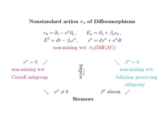
Neither of the fibre bundle constructions transforms without mixing with respect to the complementary subgroup: and mix under . Likewise and mix under . It is not hard to see that the concatenation of a Carroll- with a foliation-preserving diffeomorphisms (in either order) gives rise to a generic diffeomorphism. This suggests to search for a framework where both an Ehresmann-type connection and a shift-type co-connection are present and non-mixing transformation laws under the full Diffeomorphism group can be arranged. This is precisely what the SDiff frame (40) and the concomitant SCarroll structure (38) and (44) accomplishes. The nonstandard action of diffeomorphisms (17) on is crucial for this to work. The interrelations among the three orthonormal frames are summarized in Table 1.
3.2. Structure Functions of the SDiff Frame
Any orthonormal frame of vector fields and one forms , , has a set of structure constants associated with it, alternatively defined by or . In order to compute the structure constants for the frame , in (39) and (41) a small preparation is needed. The domain of the vectors fields must be extended from scalars to other tensors. For this is done simply by interpreting it as , where is the Lie derivative of tensors. For we contract with a generic vector to form and interpret the result as
This is a linear derivation on tensors for which one can consider the torsion
When acting on Scalars one finds
with from (50). It satisfies the key property of a torsion tensor: the form an integrable distribution iff . A similar computation gives
These results can again be specialized to , , and give
with interpreted as in (58). From here the structure constants in vector field form can be read off. Consistency requires that the same structure constants enter the exterior derivatives of the one forms . By direct computation one finds
The structure constants indeed match those in (62).
Next, we consider the transformation properties of . The result is
under the action of . The derivation proceeds by breaking up the defining relation (59) and (60) into several separately invariant pieces. To this end, we denote by the spatially projected components of two (metric-independent) vectors . They transform under according to (In the terminology of Section 4 are the spatial parts of Svectors of weight .) , , with from (22). Then will map Sscalars into Sscalars. Hence also the commutator will produce an Sscalar when acting on one. On the other hand, this commutator equals , by (60). A quick inspection shows that (64) is equivalent to the assertion that maps Sscalars to Sscalars. On account of the previous argument this will be the case iff maps Sscalars to Sscalars. With a neat Stensor calculus yet to be developed the latter has to be verified by direct computation. We first present the relevant partial results:
where we write again for readability’s sake. Clearly, (65a) and (65c) imply that maps Sscalars to Sscalars and hence (64). Further, (65c) is a straightforward consequence of (65a) and (65b) and . It remains to establish (65a) and (65b). In both computations one needs
3.3. vs. Intertwining and an Invertible Carroll Metric
The coordinate components of the SDiff frame transform under as follows
Using also the Slapse , the combinations and will transform as conventional vectors and covectors (For reoccurring symbols we use a right sub- or superscript ‘’ to indicate a ‘Carroll’ variant that depends on .)
under the action of , with invariant. So far only entered. Adjoining also one can form , and finds from (68) the standard transformation law
In summary, the induced transformation law for the quantities (69) and (70) is that of the tensorial realization. The underlying constituent fields (and indirectly ) however transform according , not according to the tensorially induced realization (A33) and (A38). This means the components and of the SDiff frame can be regarded as intertwiners between the and the realization of .
In pseudo-Riemannian metric geometry the nondegenerate metric of course transforms according to (70). The standard foliation fields are and , for a temporal function , see (A29). Suitably interpreted they also transform tensorially. Crucially, the temporal function must be held fixed to this end. For example then are the components of after a transformation. Further, N then is a scalar, so that transforms like a covector. This is to be contrasted with (A33) where N transforms nontrivially. In fact, the on the left hand side refers to a changed temporal function , namely the one would naturally use in adapted ‘primed’ coordinates. In this interpretation does not transform like a covector. Similarly, , in the second interpretation does not transform like a vector. Correspondingly has been found to transform according to (A46). In particular, is not proportional to , unless the diffeomorphism is foliation-preserving. This is to be contrasted with from (21) when computed with the realization acting on the constituent fields.
We now return to (69) and claim that the transformation laws of the constituent fields can be uniquely recovered from it:
It suffices to verify this in adapted coordinates. Then and . Reversing the computation underlying the first equation (69) one finds that holds iff transform as in (17). With this in place is found to imply (38), with the consistency condition on satisfied identically.
So far did not enter. Augmenting them one can form , as in (46). One then finds that the tensorial transformation law (70) uniquely imprints all of the transformation laws of the constituent fields:
In brief, this holds because in the relation the equations arising from the lower block fix the transformation law. Then the d relations from the off-diagonal blocks fix the transformation law. The remaining relation is satisfied identically. With this in place, the relation similarly determines the and transformations laws. In summary, the transformations (69) and (70) in combination with the defining relations in terms of uniquely characterize the nonstandard transformation laws of the latter.
This holds for the full Diffeomorphism group acting in two different ways. As before, one can now specialize to the zero Sshift gauge and transition to the ‘checked’ fields as in (55)–(57). Then is reduced to by (54). As noted after (34) the stabilizer subgroup of the zero-shift gauge with respect to the tensorial action is smaller than . Relevant in the present context is however the specialization of the transformation laws (68)–(70) induced by the action. This is readily seen to be the subgroup of , acting tensorially. The intertwining relations (68) specialize to
Evaluating these in adapted coordinates with , , , , one finds that and , necessarily have to be of Carroll type: , , . The previous characterization of the nonstandard transformation laws in terms of the standard ones therefore carries over upon restriction to the Carroll subgroup: the checked versions of (69) and (70) intertwine the realization (55) and (56) and the realization of the Carroll group.
Invertible Carroll metric. One might be tempted to view the degeneracy of the Carroll metric in (44) and (45) as the hallmark of the augmented Sgeometry. However, with the same data one can define an invertible metric. Consider
with , from (69). Both are invertible, , and the induced transformation law is
Hence, an SCarroll structure on a manifold can be used to endow the same manifold also with a pseudo-Riemannian metric. Moreover,
holds, making the SDiff frame a metric frame with respect to . Indeed, the structure of (74) mirrors that of and in pseudo-Riemannian geometry, see (A28) and (A29). Similarly, (76) is parallel to (A26) and (A50).
In order to explore the parallelism further let us try to equate
This gives rise to an overdetermined system of equations that allows one to express the metric data in terms of the Carroll data. Explicitly
Consistency requires that the Sgravity transformation laws (17) and (22) combined with that of the SEhresmann connection (38) imply the tensorially induced ones for in (A33) and (A38). This is indeed the case, as can be verified by straightforward computations. Recall from (48) that the SEhresmann connection can be realized in terms of a scalar field, . The correspondence (77) and (78) then defines an intriguing notion of a ‘composite metric’.
The map cannot be invertible, as the degrees of freedom have no counterpart. A trivial one-to-one correspondence can be set up in gauge. This reduces the group to its foliation-preserving subgroup , and both sets of fields simply coincide: , , , . A more interesting one-to-one correspondence arises in gauge. As seen earlier, this reduces to and the induced action is via the subgroup of . Denoting again the Sfields in the gauge by a check one finds
By construction the action on the Sfields induces the specialization of (A33) and (A38) for . Conversely, given carrying the tensorially induced transformation law , one can view (79) as the definition of certain composite fields. The assertion then is that the composite fields have the simple transformation laws (55) and (56). In this reading the relations (79) are implicit in [5,6] when the Randers-Papapetrou form of the line element is matched to the ADM form. The interpretation as a gauge fixing of (77) and (78) with the underlying fully diffeomorphism covariant invertible is new.
First order frames. All frames considered so far block diagonalize the respective metric. In first order formulations typically ‘Vielbeins’ are used which diagonalize the underlying metric, see [14,15] in the present context. Such frames can be obtained from the ones considered simply by diagonalizing . We return to (26) and rewrite it in terms of . The reasoning leading to (26) also applies to and gives rise to its normalized, mutually orthogonal eigenvectors , . Together
The spatial parts of the frames considered can then be redefined
and give rise to an SVielbein, an SDiff Vielbein, and (by setting ) a Carroll Vielbein. Orthogonality and completeness holds in the form
while orthogonality with the respective temporal parts is preserved. Both the degenerate and the nondegenerate Carroll metric are diagonalized
4. Stensor Calculus
We now aim at developing a tensor calculus which bears to Sgravity and its diffeomorphism invariance an analogous relation as Einstein gravity in form has to its non-manifest diffeomorphism invariance. For example, the standard tensor calculus is designed such that the Einstein tensor is a symmetric type tensor, although less manifestly so in form. The counterpart of the Einstein tensor in Sgravity does not transform like a conventional tensor. Yet, on account of the full diffeomorphism invariance of the underlying action some adapted notion of an ‘Stensor’ ought to exist.
Our basic approach is via the limit construction (4) outlined in the introduction. We elaborate on it in Section 4.1, proposing a broad but implicit and a narrower but more intrinsic notion of an Stensor. In Section 4.2 we consider the linearized transformation laws of Stensors and exemplify the concept with the counterparts of the metric, the Einstein, and the energy–momentum tensor in Sgravity. In Section 4.3 we show that the weight-dependent transformation laws can always be brought into a simple standard form (in which the blocks do not mix) by means of a ‘decoupling transformation’. The latter makes crucial use of the SCarroll structure introduced in Section 3.1.
The scale transformation in (4) refers to a choice of foliation but is insensitive to foliation-preserving diffeomorphisms . We thus fix a fiducial foliation and choose some orthonormal frame , adapted to it. We will frequently encounter tuples of tensors that arise as the components with respect to some such frame, regardless of its transformation properties under foliation changing diffeomorphisms. A convenient definition is:
Definition 2.
(1+d tuple).On a foliated manifold M let , be an orthonormal frame transforming covariantly under ,
No transformation properties of the frame under foliation changing diffeomorphisms are assumed. Let be the coordinate components of a conventional type tensor and consider (in some lexicographic ordering) the set of all obtained by contracting with copies of , copies of , and copies of , copies of . A tuple is a tuple , of tensors with the index structure implied by the above contractions. The convention for the labeling is such that .
Since for each lower and upper index there are two choices at most -independent tensors arise. If U has symmetries the number of independent blocks could be smaller. By construction
One could easily spell out for each type the index structure of the tuples explicitly. Then reference to an underlying conventional tensor could be avoided. In the following we consider the tuples obtained by taking as the frame one of the previously studied frames: the metric frame, the Sframe, and the SDiff frame. We begin with the metric frame.
4.1. Limit Construction of Stensors
We return to the intertwining relations (A48) of the metric frame. As exemplified in (A52) and (A53) one can use them to determine the nonlinear transformation law of tensor components with respect to the , orthonormal frame. We now consider the scaling limit of this construction.
Stensors of weight zero. On a foliated pseudo-Riemannian manifold consider the tuple , obtained by taking the metric frame components of a conventional type tensor U and assume the to be invariant under from (13). The limit (4) then always exists with zero weights, . The tuple with the transformation law , , imprinted by the limit is called an Stensor of type and weight zero.
In pseudo-Riemannian geometry conventional tensors that are independent of the spacetime metric give rise to Stensors of zero weight. However the metric-independence is not a necessary condition, only the -invariance of the with respect to the fiducial foliation matters. Under these conditions the existence of a limit with in (4) can easily be seen from the intertwining relations (A48) of the metric frame. As long as the metric frame components of the conventional tensor considered are invariant, the only nontrivial response in to the scaling (13) is the replacement of with in the intertwining relations (A48). In the limit the -dependent terms in (A48) drop out, resulting in the intertwining relations of the Sframe
In the limit the metric shift should be replaced with and the components in (86) can be viewed as referring to the Sframe expanded in a generic coordinate basis: , , , . The relations (86) can then also be computed directly from (17) without referring to (A48) and its scaling limit. The invariance of the orthonormality relations (A49) carries over to the Sframe. The relations (86) witness again two remarkable properties: the and components do not mix with the other frame components under the action, and the transformation pattern is independent of the spatial metric and its inverse. The intertwining relations (86) can be used to compute the transformation law for any weight zero Stensor, without reference to the limit construction.
For the sake of illustration we consider vectors and covectors here; the extension to tensors of arbitrary rank and type is straightforward. Consider first the -invariant Sframe components of a vector field . Then
Similarly, the -invariant Sframe components of a covector transform according to
The same transformations arise by taking the scaling limit of (A52) and (A53). Expressed in terms of the Sframe components the vectors fields and one-forms read
This highlights again the intertwining character of the construction: the left hand sides are invariant under the standard tensorial action of diffeomorphisms while the right hand sides are invariant under the action.
A type Stensor of weight zero is called an Sscalar, and examples have already been encountered in the verification of ’s invariance. A simple example of an Scovector arises from the gradient of a metric-independent Sscalar like . In adapted coordinates the components are , ; hence , are its Sframe components. By direct computation one finds this pair to transform according to (88). Hence, is an Scovector of weight .
Other Stensors of zero weight can be formed by taking tensor products. In addition, Stensors of zero weight admit a trace operation inherited from conventional tensors that commutes with taking tensor products. Both aspects will be detailed below.
Stensors of integer weight. Often the existence of a nontrivial limit in (4) requires nonzero weights, . We begin with a broad but somewhat implicit definition
Definition 3.
(Stensors as Limits).On a foliated pseudo-Riemannian manifold, a tuple , , of tensors is called an Stensor of type and weight , if it arises from the metric frame components of a conventional type tensor as the finite nonzero limit . Then
defines its transformation law, which depends only on the type and the weights. In the limits the substitution is understood. Whenever unambiguous the “” left superscript will be omitted.
Several features are implicit in this ‘Limit Definition’: first, nonzero weights arise only if the conventional tensor U is metric-dependent. Second, the mixing pattern of the components can be computed from the intertwining relations (A48) by keeping only the leading terms in a large expansion and it is uniquely determined by the type and the weights . The discussion after Equation (A53) implies that each is a linear function of the , , while may enter nonlinearly. Third, for a fixed type only a finite number of consistent weight assignments exist, see Section 4.2.
While the Limit Definition successfully defines the realization for generic tensors it does so non-autonomously in terms of . For most purposes the Limit Definition is also too broad. In order to motivate a narrower but more intrinsic notion we begin with the following observation: the metric frame components of a conventional tensor U some of whose indices have been moved with will differ from those of an underlying tensor V with scale invariant metric frame components solely by having some of the indices moved with . This covers most of the situations occurring in gravitational fields theories. The -invariant combinations may include derivatives of like or , etc., but terms with nonzero scaling weight then normally arise from moving indices with the undifferentiated spatial metric. In the following we restrict attention to ‘metric compatible’ Stensors arising as the weighted limits of conventional gravitational tensors of this form. In this situation the weights are always even integers and the Sframe components are related to those of an underlying Stensor of zero weight by moving indices with .
Definition 4.
(Metric compatible Stensors).Let M be a manifold foliated by the fields entering the Sframe (36) and equipped with transforming according to (17) and (22). A tuple , of tensors is called a metric compatible Stensor of type and weight , if it arises from an Stensor , of the same rank but zero weight by moving indices with . Metric compatible Stensors arising from variations of the Sgravity action will be denoted by a subscript ‘0’.
This is an intrinsic notion in that no reference to the scaling is made. A minor indirect reference to conventional tensors is made through the notion of a tuple. The latter also entails that the occur coordinated in different blocks in a way compatible with moving spacetime indices with . As a consequence the always originate from the scaling limit of at the same position in the tuple which ensures consistency with the Limit Definition. As in the definition of an tuple, the reference to conventional tensors could be avoided by listing the possible patterns that can arise. In any case, the resulting are constructed from , suitable derivatives, and the underlying components. The scaling degree of some such can be read off simply from that of the constituent fields: , , , . Further, the transformation law of the can be computed intrinsically from the realization alone, and thus does not have to be part of the definition.
As an illustration, consider again the case of a vector and a covector with -invariant metric frame components. Then defines a covector, whose metric frame components , are related to those of by , . The components will transform according to (A53). However, now transforms nontrivially under the scale transformation (13). As a consequence the scaling limit of (A53) is not given by (88) but rather by (92) below. Similarly, defines a vector whose metric frame components , , are related to those of by , . Before scaling transform according to (A52). However, since under (13) this will again affect the scaling limit. Instead of (87) the limit of (A52) is now given by (93) below.
The interrelations of the Sframe components will be the same, just with replacing . By Definition, the tuple is a metric compatible Scovector of weight and is a metric compatible Svector of weight . The relations to the underlying weight zero Svector and Scovector are given by
The transformation laws can be computed using only the realization, i.e., (17), (22), (87) and (88), and coincide with the ones obtained via the limit construction:
Scovector of weight (0,2):
Svector of weight (0,−2):
One may verify that the inner product, , is invariant. Note that the transformation pattern (92) and (93) clearly differ from those of the weight counterparts in (88) and (87), respectively.
Tensor product. A basic operation for conventional tensors is the tensor product. In view of (90) one may ask whether the scaling limit of a tensor product coincides with the tensor product of the limits and defines again a weighted Stensor. This is indeed the case and can be seen as follows. Let U be a conventional type tensor which factorizes into a tensor product , i.e., , in terms of coordinate components, for , . Its metric frame components are obtained by contracting with in all possible ways and therefore factorize as well: , , where we now interpret the indices as abstract ones and correspondingly include the tensor product symbol. The weights are additive, , and we may assume them to be such that the limits , , exist separately, i.e., there are no spurious cancellations in the product. The standard realization of the diffeomorphism group is such that , for all , whence named ‘tensorial realization’. It follows that
The same holds for the linear hull of expressions of the form , which concludes the argument.
The weighted Stensors of a given type obviously form a linear space. The above result shows that they can also be endowed with a tensor product under which the weight is additive
The resulting tensor algebra has as its automorphism group. Symbolically,
in analogy to the standard case (A15).
We add some comments: (i) Importantly, the weighted Stensors do not in general admit a well defined trace operation. In particular, is not equipped with a trace operation. The qualified existence of a trace operation and the circumstances under which it commutes with taking tensor product will be discussed below. (ii) It is not automatic that all weighted Stensors can be obtained by taking the linear hull of tensor products of Svectors and Scovectors. Examples will be discussed later on. However the transformation laws of generic weighted Stensors can be obtained from (87) and (88) alone by taking tensor products. (iii) An exception to (i) and (ii) are Stensors of weight zero. These always admit a well-defined trace operation that commutes with taking tensor products. Moreover, for weight zero all higher rank Stensors can be obtained by taking tensor products of rank one Stensors. Both properties follow from the Sframe intertwining relations (86).
Trace operation. The tensor product (95) applies to all weighted Stensors, in particular to metric compatible ones. One will naturally want a trace operation to be compatible with moving indices; so we restrict attention to metric compatible Stensors. Then only trace operations contracting a covariant with a contravariant index need to be considered. To motivate the definition we return to conventional tensors and their metric frame components. Before taking the metric frame components contraction with effects the trace over a lower index and an upper index. The completeness relation for the metric frame reads
see (A25) and (A26). It can be used to expand any type conventional tensor U in terms of its metric frame components , see (A54). The trace will likewise be governed by (97) and produce the expansion of a type tensor. The coefficients of the latter will be linear combinations of spatial traces of a subset of the original coefficients . We write for the coefficients , assuming that it is clear from the context over which pair of indices the trace is taken. For example, a type tensor with without symmetries and components will expand into 8 terms, while the trace expands into 2 terms with coefficients that involve spatial traces of only 4 of the original 8 coefficients. Explicitly
The Stensor of weight associated with U has components . Whenever well-defined we define its trace by the same spatially contracted linear combinations as the original tensor. In the above example, the trace of the type Stensor , has the 2 coefficients , , where , , , , are the limiting counterparts of the coefficients in (98). A necessary condition for this to make sense is that all terms in a linear combination have the same weight. In the example must have weight 0 since has, and and must have the same weight. Generally, in each linear combination all terms must have a fixed weight, for which we write , . If the original Stensor has weight zero this is automatically satisfied, otherwise this condition restricts the class of weighted Stensors which allow for a well-defined trace. Whenever this condition is met, one will want the tuple to transform as an Stensor of type and weight . This will normally be the case automatically but is best verified on a case-by-case basis.
In summary, for any Stensor of type and weight one can (for a pair of indices understood) introduce the tracial coefficients , , as a linear combination of spatial contractions of the original coefficients . Assume that the terms in each linear combination carry the same weight and that the set , transforms like an Stensor of type and weight . Then the latter Stensor is called the Strace of , .
A relevant example is the SRiemann tensor (124) below, which can be modeled as an Stensor of type and weight . Its Strace then is a type Stensor of weight , which coincides with the independently defined SRicci tensor.
Generally, Stensors of weight zero admit a trace. The condition on the weights is trivially satisfies so that only the transformation law needs to be checked. As far as the transformation law is concerned we can model the Stensors in question as a tensor product of Svectors and Scovectors of zero weight. Since all indices are on the same footing it suffices to verify that the type Stensor admits a trace. The trace is given by and ought to transform as an Sscalar, based on (87) and (88). This is indeed the case. It follows that for zero weight the tensor algebra can be equipped with a trace operation that commutes with taking tensor products, in exact analogy to the standard case.
4.2. Examples of Stensors and Their Gauge Variations
In the second half of this section we present prime examples of Stensors relevant in a gravitational context. Among them are Sgravity counterparts of the metric, the Einstein- and energy–momentum tensor, as well as the Riemann tensor. All of them are metric compatible Stensors in the sense defined and are subject to a specific weight-dependent transformation law. Those related to variations of the Sgravity action will be denoted by a subscript ‘0’ rather than a left superscript ‘’.
For many purposes the linearization of transformation laws under generic diffeomorphisms suffice. For standard tensors on some smooth manifold M this is implemented by the (generally covariant) Lie derivative. If M is a foliated pseudo-Riemannian manifold the latter induces gauge variations on the metric frame components that are discussed in Appendix A.3. Here we aim at counterparts of these gauge variations for Stensors.
A convenient starting point is the linearized version of the Limit Definition. Consider the tuple , of tensors obtained by taking the metric frame components of a conventional tensor. The tuple transforms under infinitesimal diffeomorphisms according to the gauge variations induced by the spacetime Lie derivative. We write , for these gauge variations and take their scaling limit. By assumption each scales according to and the right hand side of may also explicitly depend on , . As a results there are for each type only a finite number of weight assignments , that lead to a consistent nontrivial limit. These can readily be classified and lead to a list of possible linearized transformation laws for Stensors in the sense of the Limit Definition. We write for these Stensor gauge variations and label them by the weight tuple , . Whenever unambiguous the “” left superscript will be omitted.
Not all of these cases are compatible with moving spacetime indices as required for metric compatible Stensors. In a second step one can screen the previous list for compatibility with these criteria to obtain a subset of possible weights and linearized transformation laws metric compatible Stensors. We illustrate the construction for rank .
For rank 0 there is only one possibility: rank 0 tensors are scalars and their counterpart has already been introduced. Infinitesimally
characterizes Sscalars.
For rank 1 there are four consistent limits:
Scovector, weight :
Scovector, weight :
Svector, weight :
Svector, weight :
These are precisely the linearized versions of (129), (130), (92) and (93). On account of (91) all four cases are also metric compatible.
The list of transformation laws for rank two Stensors arising as weighted limits can similarly be generated by inspection of (A62), (A65) and (A68). The results are collected in Table 2.
Most of these are not metric compatible. In the following we focus on three cases directly relevant for Sgravity: covariant symmetric rank two tensors of weight ; contravariant symmetric rank two tensors of weight ; and the interpolating case of a mixed rank two tensor of weight zero. We first note the transformation laws, which can be obtained, for example, from (A68), (A65) and (A62).
Type , weight , :
Type , weight , , , :
Type , weight , :
We yet have to show that the two symmetric Stensors are indeed metric compatible in the sense defined. In order to do so, we note that the transformation law (105) is consistent with the following reduction conditions
The reduced transformation law reads
with . In terms of the reduced weight zero Stensor we define , , . Then transforms according to (104). By Definition it is a symmetric, metric-compatible Stensor of type and weight . For the contravariant case one proceeds similarly. In terms of the reduced weight zero Stensor one defines , , . Then (108) implies that transforms according to (106) and hence defines a symmetric, metric-compatible Stensor of type and weight .
Another aspect of the metric compatibility of and is the existence of a well-defined trace operation inherited from the underlying mixed weight zero Stensor. For the latter the trace operation is a special case of the one described after (97). Explicitly, , which transforms like an Sscalar. Using the above construction one obtains the induced trace operations
These expressions adhere to what one would expect from the completeness relations (A61) and (A67) and are Sscalars on account of (104) and (106). These mathematically preferred cases turns out to be also the ones for which Sgravity provides constructible examples.
Sgravity metric as an Stensor. The projected components of the pseudo-Riemannian metric are , and the transformation law (A68) specializes consistently. The Sgravity metric will naturally be assigned projected components , and as such should be a type Stensor of weight . The transformation law (104) indeed specializes consistently. Moreover, the nontrivial variation, , coincides with the one in (19). Note that the nontrivial weight assignment is essential for this to work. The strong coupling contra-metric will similarly be assigned projected components . As such it should be an Stensor of type with weight or . On account of the preceeding discussion we take the weight to be . The transformation law (106) indeed specializes consistently and the nontrivial variation, , matches the linearized form of (22). Both and have a well defined trace (109) which equals .
Energy–momentum Stensor. Next, consider the energy–momentum tensor of the scalar field (A69). In order to take the scaling limit we interpret the scalar field as dimensionless and scale invariant as in (13). For the limit of the energy–momentum tensor’s components one then finds
Here ‘subst’ refers to the substitution (16) and the limits are viewed as functions of . In parallel to (112) below the limiting expressions can alternatively be obtained as variations of the matter part of the action in (1); keeping to our notational conventions we therefore denote them with a subscript ‘0’. Along different lines this matter action also arises in a first order formulation [15]. Based on the previously defined transformation laws one finds by direct computation
This agrees with the transformation law (104) of a type Stensor of weight . Since the last equation in (111) is equivalent to . This pairs with the first equation, as . It also ensures that the scaling limit of the trace in (A69) transforms like a Sscalar under .
Field equations Stensor. The gauge variations of the purely gravitational part of the strong coupling field equations must be compatible with (111). In general relativity this is ensured by the transformation properties of the projected components (A72) of the Einstein tensor. In Sgravity we define
with from (1). This parallels (A72), but since is regarded as a functional of (not ) the sign in the second term of is flipped. Taking this into account, the expressions (112) turn out to be the weighted scaling limits of the Einstein tensor’s components in the metric frame:
As a consequence should transform as an Stensor of type with weight . Explicitly,
It is a nontrivial consistency check that this comes out correctly, based solely on the variations of the basic Sgravity fields and the definition (112). Before turning to this check, observe the difference to the transformation law (A68) satisfied by the projected components of the Einstein tensor: in contrast to (A68) the mixing only occurs in the variation. Importantly, (114) matches (111) in the matter sector which renders the Sgravity field equations
foliation-independent.
We now turn to the direct verification of (114). A bonus feature is that the result turns out to be valid for arbitrary parameter c in the DeWitt metric, i.e., when in (12) is replaced with . The limit of Einstein gravity corresponds to . In order to facilitate comparison with (A72) and [1,10] we regard as a functional of and the densitized Slapse instead of . We write for the resulting c-dependent purely gravitational part of the Sgravity action (12), with ‘L’ indicating that the Lagrangian not the Hamiltonian version enters. For simplicity we also omit the cosmological constant term, which can be restored from the previously treated matter sector by shifting the potential, . In this setting the independent variations are: (the Lagrangian form of the Hamiltonian constraint), (the Lagrangian form of the Diffeomorphism constraint), and . We first note the explicit forms of
Since , all constituent quantities transform according to their Lie derivatives under purely spatial gauge transformations. Hence also and , transform according to their spatial tensor type (a scalar density and a cotensor density, respectively) under time-dependent spatial gauge transformations. For the temporal part of the gauge transformations we use as the descriptor, matching . A lengthy direct computation then shows
Unlike in general relativity, the evolution equations do not mix with the constraints and thus could be imposed separately. The gauge variation of requires variation of the Christoffel symbols. A slightly more efficient route is to start from the averaged form
for a non-dynamical spatial vector . In the gauge variation of (118) one finds that the terms cancel and that modulo total time derivatives the result can be written as the spatial average of . Stripping off the auxiliary vector one obtains
It is instructive to compare this with the Diffeomorphism Ward identity for pure Sgravity
where the · indicates a integration. Stripping off the gauge descriptors yields
Specializing (119) to thus mirrors the time evolution of , as expected on general grounds. The second equation in (121) can also be used to rewrite (120) in a more suggestive form
SRiemann tensor. Rank four Stensors warrant a systematic discussion, omitted here. Mostly in order to highlight the difference to other notions of curvature we present the scaling limit of the Riemann tensor. We begin with noting the metric frame components of the type Riemann tensor
Here the superscripts refer to the scaling weight of the homogeneous parts under the scaling transformation (13). As before, is the extrinsic curvature. Since all blocks are built solely from there is no freedom to choose weight assignments. A nontrivial limit for the blocks arises only for the case
In line with the general conventions we changed the notation in the limiting quantities and regard them as functions of . Note that the dependence on the Riemann tensor of the spatial metric has dropped out. The Riemann type symmetries are preserved in the limit and imply
Together with the transformation law (127) below the weights in (124) identify the quadtuple as a (specific) Stensor of type and weight . We shall refer to it as the SRiemann tensor.
The SRicci tensor is defined analogously, starting from the contractions of (123). Its transformation law is that of a type Stensor of weight , which can be obtained by taking the weighted limit of (A65). On the other hand, one can take the trace of the limits (124) and finds
These coincide with the indicated coefficients of the SRicci tensor, rendering the transition from (126) to (126) an example of an Strace, as previously discussed.
The transformation law under infinitesimal transformations for type Stensors of weight and with Riemann-like symmetries are as follows
4.3. Decoupling Maps
So far the covariant Carroll structure of Section 3.1 did not enter. Making use of it, the transformation law of metric compatible Stensors can be coded in a more concise way.
Weight zero. Stensors of weight zero can be viewed as arising from some conventional tensor by taking components with respect to the Sframe, written as , which turn out to be invariant. This leads to a characteristic mixing pattern for the blocks that can be inferred from the Sframe intertwining relations (86). On the other hand, one can consider the components of the same conventional tensor with respect to the (-rescaled) SDiff frame, , . Concretely, for a type tensor with coordinate components the components arise by contracting in all possible ways with . For clarity’s sake we denote the components with respect to the SDiff frame systematically by a left superscript, . In particular, a left superscript does not necessarily signal a dependence as before.
On account of (68) the multiplets do not mix under arbitrary transformations. The tuples and , , can be related by expressing one set of frame coordinate components in terms of the other. Using the rescaled variants and (39) and (42) the nontrivial conversion formulas are
For example, in the case of a vector field with -invariant Sframe components one has
For a one-form with -invariant Sframe components one finds similarly
Compared to (87) and (88) the mixing terms have disappeared. For later reference we also note the transition formulas for a weight zero Stensor of type :
Again, the affine transformation law precisely cancels the mixing terms of the original Stensor blocks. This holds generally:
Consider the tuple , , obtained by taking the SDiff frame components of a conventional type tensor U, and assume them to be -invariant (treating as invariant). Each of these SDiff frame components transforms multilinearly among itself for fixed , with for each lower a index, and with for each upper b index, while contractions do not affect the transformation law. Further, each can be expanded in terms of the Sframe components , for varying , with -dependent coefficients. As a consequence the decoupled transformation laws for the SDiff frame components are in one-to-one correspondence with the mixing transformation law of the Sframe components.
Nonzero weight. Next, we seek to generalize this correspondence to Stensors of nonzero weight. The tuple , , obtained by taking the SDiff frame components of a conventional type tensor U, will then no no longer be -invariant. One may be tempted to simply take the weighted limit , to obtain the nonmixing multiplets. Some experimentation shows that this does not work; the limits in general do mix under transformations.
Instead, we proceed as follows. Restricting attention to metric compatible Stensors the idea is simply to apply the decoupling map of the underlying Stensor of zero weight and rewrite it to obtain a decoupling map for the weighted Stensor. We first illustrate the procedure with several examples.
Consider a weight zero Scovector and define . As seen before, then transforms as an Svector of weight . Applying the decoupling map (130) to , i.e., , , and rewriting it suggests
By direct computation one can verify that (132) indeed decouples the weight transformation law (93). Similarly, starting with a weight zero Svector one can define , . Then is an Scovector of weight . Applying the decoupling map (129), i.e., , , gives
These can be checked to decouple the transformation law (92). In fact, the original and the decoupled transformation laws are in one-to-one correspondence.
We remark that both maps (132), (133) can alternatively be obtained by moving the spacetime index with the invertible Carroll metric (74) to get and , in a first step. The SDiff frame components of are given by , . Utilizing the weight zero map (129) and inserting the definitions reproduces (132). Similarly, the SDiff frame components of are , . Utilizing the weight zero map (130) and inserting the definitions reproduces (133).
Next we consider rank 2 metric compatible Stensors and focus again on the two cases from Section 4.2. We first present the decoupling maps in both cases and then comment on the derivation:
Type weight :
Type weight :
In Section 4.2 we noted explicitly the linearized form of the transformation law for each of these weighted Stensors. It may suffice here to verify the decoupling property also at the linearized level. The additional variation needed is the linearized form of (38) which comes out as
Using (104)–(106) and (136) one can verify that the given combinations indeed decouple the linearized transformation laws, that is, (138) below holds.
In order to derive (134) we return to the realization of in terms of the reduced type Stensor of weight , with . One has , , . Next, we recall from (131) the decoupling map for a weight zero type tensor. Specializing to , and inserting the defining relations for one obtains (134). The derivation of (135) proceeds similarly. In term of the reduced weight zero Stensor one realizes as , , . The decoupling map (131) specialized to implies (135).
The construction principle generalizes and yields the following result and definition:
Definition 5.
(Decoupling map and SCarroll tensor).Let , be a metric compatible Stensor of type and weight . Then there exists a homogeneous polynomial of degree in , , and possibly preexisting Stensors such that
decouples the transformation law. The map is called the decoupling map and the resulting tuple , is called an SCarroll tensor of weight .
We add several explanations. (i) The degree is defined by , , , . (ii) By a decoupled transformation law we mean that each transforms multilinearly among itself under generic (foliation-changing as well as non-Carroll) diffeomorphisms in the realization, where an occurs for each upper and a occurs for each lower index. The component is always invariant. Upon linearization this amounts to
where is the d-dimensional Lie derivative acting on according to its tensor type. (iii) The term SCarroll tensor is modeled after that of Carroll tensors [5,9] which transform covariantly and without mixing under the Carroll subgroup of diffeomorphisms. SCarroll tensors have the same feature but with respect to the realization of the full diffeomorphism group. In fact, an SCarroll tensor gives rise to a tuple of Carroll tensors by fixing the gauge. For SCarroll tensors of weight zero this is clear from the reduction of the corresponding frames, see (57). In particular, each upper index transforms with and each lower index with . The same holds if indices are subsequently moved with or as they transform correspondingly under the Carroll subgroup. (iv) The SCarroll tensors are a convenient arena on which an adapted Levi–Civita type connection can be defined, see Section 5.3.
5. Sconnections
The nonstandard transformation laws (21) of the Sgravity metric blocks does not allow for an interesting notion of spatio-temporal parallel transport. A purely temporal partial connection exists however which has a transparent relation to the scaling limit and a symmetrized Bott connection. By utilizing the SEhresmann connection and the decoupling map also a fully covariant SCarroll–Levi–Civita connection can be introduced.
5.1. Connections in Orthonormal Frames
For convenience we collect here the main formulas for the connection formalism in orthonormal frames. Initially we take M to be a -dimensional differentiable manifold equipped only with an orthonormal frame and consider the frame components of tensors. Next we augment a generic affine connection which we later specialize to be metric and torsion-free. Finally, we illustrate the use by application to the Levi–Civita connection in the metric frame, as needed later on.
Let , be a “frame”, i.e., a basis of in general non-commuting vector fields on M, , and let , be the dual 1-forms, . Using for the differential of a one-form one has
Expansion in a local coordinate basis gives the “vielbeins” , , with , . Coordinate components of a tensor U can be converted into frame components .
Generic affine connection: An affine connection ∇ assigns to every vector field V a derivation that preserves the tensor type, obeys for scalars f, and commutes with contracted multiplication. The coefficients of an affine connection ∇ with respect to a frame are introduced by
with . On the frame components of a tensor , the covariant derivative then acts by
The torsion and curvature of ∇ are defined by , and , respectively, for vectors fields . The definitions imply the Cartan structure equations
where is the connection one-form and the two-forms on the lhs were expanded in terms of the frame components , . Explicit expressions for them can be obtained either directly or from the structure equations, with the result
Detailed derivations can be found, e.g., in [34], Sections 13.5–13.8. The structure equations imply the Bianchi identities which in turn project onto component identities
where the sums are over the cyclic permutations of the indices.
Next, consider a change of frame basis
for some function . In the ‘hatted’ frame the connection components are defined by , with . Relating this to the original defining relation (140) one finds
This alone implies that the covariant derivative’s frame components (141) transform covariantly
Since the torsion and the curvature are defined in terms of only, their frame components will transform covariantly as well under a change of basis.
Torsion-free metric connection: So far no metric entered. If M is in addition a pseudo-Riemannian manifold with metric g and ∇ is a metric compatible connection, i.e., , one has explicit expressions for the connection coefficients in terms of , , . The metric compatibility translates via and into
which combined with also fixes the symmetric part of . Together
Next, we specialize to a torsionfree metric connection, which is unique and called the Levi–Civita connection. Then (149) holds with . More directly one can obtain this from the solution of . and , in terms of the Koszul formula
see, e.g., [34], p. 590. It can be evaluated in any basis of vector fields , , using only the defining relations , , where . The result is again (149) with . In a coordinate basis , , the connection coefficients (149) then reduce to the Christoffel symbols . The relation to the connection coefficients in a generic frame is given by
This is such that .
Levi–Civita connection in metric frame. In order to apply this to the metric frame we identify
where we momentarily use a breve to distinguish acting on scalars from the general acting on arbitrary tensors. The dual one-forms are normalized according to . The frame components of the metric are . The nonvanishing commutator coefficients are
The torsion vanishes by definition, . For the connection coefficients one finds from (149) initially expressions where time derivatives enter through . Rewritten in terms of , one obtains
The general formula (141) then determines the metric frame components of in terms of U’s metric frame components, for any (directional) vector W. The covariance under the standard tensorial action of diffeomorphism is accounted for by the general transformation formulas (146) and (147). The relevant B matrix corresponds to the diffeomorphism induced reorganization of the metric frame and can be read off from (A46) and (A33a) and the transformation formula in (37) (which applies to the metric frame as well, up to a change in notation). The B matrix has no zero entries and the component instances of (146) are unenlightening. The component form of (147) is best elucidated in the scalar and rank one case.
In fact, a covariant (directional) derivative can be introduced axiomatically as a derivation of the tensor algebra, see, e.g., [34], Section 13.4. As such it is uniquely determined by its action on scalars and (co-)vectors. In this approach we seek to characterize by its action on scalars and (co-)vectors. The direction is normally described in terms of a vector (); for later use we also prepare a covector version (). In both cases the metric frame components are used, for and for . Acting on a scalar one then has
By construction, are the frame components of a covector which implies that transforms like .
The corresponding relations for vectors with metric frame components and covectors with metric frame components read
By common abuse of notation we write , as , and similarly for the other components. Further, is the extrinsic curvature, and indices are moved with . In the derivation, one starts from the vector and covector version of (141) and inserts (154). Initially again the scalar derivative enters, which has been converted into the proper Lie derivative action of in order to arrive at (156).
We add several remarks: (i) The characteristic properties of an affine connection manifestly hold: directional linearity and the Leibniz rule , for all scalar functions f. (ii) As a check one may verify that (upon conversion , ) acts on like a scalar, see (155). (iii) The vector and covector versions are related by moving indices,
subject to the identifications , , , . The relations (157) in turn are consistent with . The latter is a special case of ’s action on a rank two tensor. (iv) Generally, the action of on the metric frame blocks of some type tensor can be computed either from (141) or by considering tensor products of the (co-)vector actions (156). (v) The specialization of (156b) leads to a form of the geodesic congruence equation. Explicitly, iff
5.2. Temporal Covariant Derivative from Scaling Limit
Since a covariant derivative maps tensors to tensors, the limit construction (90) can be applied before and after taking the covariant derivative. We wish to study the induced relation of the limits.
We recall from Section 4.1 that for a vector there exist two consistent weight assignments for its metric frame components , namely or . Similarly, for a covector only two weight assignments for its metric frame components lead to a finite nonzero limit, namely and . As before, both versions related by , and the zero components always have weight zero. On account of (157) we may therefore restrict attention to the limits of (156b). In line with the general convention, we attribute to scaling weight zero; deviating from it would remove the temporal transport term, at odds with the interpretation of as a derivation. By inspection of (156b) one sees that only two weight assignments for the covector pairs lead to finite nonzero limits. For convenient reference we also note the limits of the conjugate vector versions. Case one is:
Case two is:
In both cases the ‘directional” covector has weight zero and the image has the same weight as . Only (159) admits a specialization, which produces the geodesic congruence equations of strong coupling gravity [35]. In line with the conventions of Section 4.1 we shall replace with their Sgravity counterparts , after the scaling limit has been taken. In particular, with after the substitution.
In order to interpret the limits of in (159) and (160) as connections directional linearity and the Leibniz rule should hold. While directional linearity is valid for all the Leibniz property works only if or the scalar f is a function of t only. We adopt the first restriction and note
valid for all . This suggests to interpret the limits of (159) and (160) as partial connections. These can be defined for any vector bundle and distribution over a manifold, see, e.g., [37] in a related context. Here we consider directly the tangent bundle and an integrable subbundle . The annihilator of is the subbundle of the cotangent bundle consisting of one forms that vanish on . Then is a partial connection in along if , and hold for all scalars f and , .
Identifying with the temporal subbundle of generated by and with the spatial one forms in , this concept applies to the situation at hand and we write for the resulting partial connection. The directional vector just occurs as a prefactor , for . The ‘temporal’ directional derivative itself corresponds to . Its defining relations can be read off from (159) and (160) and read
where and (161) ensures the defining properties for both weight assignments (159) and (160). Similarly, one can define a partial connection acting on vectors
again for both weight assignments. The vector and the covector version are related by moving indices
Equivalently, is metric compatible in the following sense
Another natural partial connection on the (co-)tangent bundle is the Bott connection, see, e.g., [4,37,38]. In the above notation the defining relations are
The covector version is related to the vector version by the usual formula; both enter in the following. In order to evaluate (166) with the previous identifications, we prepare the metric frame components of the commutator
For the metric frame components this gives explicitly
After renaming of the Bott connection thus evaluates to
with . Again, the directional vector only occurs as a prefactor and it suffices to consider the case for which we write . The Bott connection is not compatible with moving ‘spatial’ indices, rather there is an induced action of the covector version on vectors and of the vector version on covectors given by
Comparing with (163) and (166) one sees
on spatial vectors and covectors; see also [38]. The symmetrization accounts for the metric compatibility (165) of noted before.
Next we verify the covariance properties of . Since the directional vector transforms as well we consider . On account of the definitions (162), (163) the image of a spatial (co-)Svector should transform again as a spatial (co-)Svector of the same weight. Since always has weight and its transformation law is imply . For the (co-)vector acts on there are two cases to consider: can have weight or ; similarly can have weight or . The transformation laws in general mix the spatial with the temporal component, see Section 4.1. In precisely those cases where the spatial component mixes on can, however, set the temporal component to zero consistently, thereby obtaining a non-mixing transformation law. Specifically, the pattern is as follows:
Similarly,
Here is defined in (22) of and obeys (23) as well as . The transformation laws of the images of various quantities have been prepared in (28) for ; (27) for ; (65b) for . These imply the desired results:
where in order to be consistent with (172) one should define
In summary, the definitions (162) and (163) provide for rank one Stensors an intrinsically defined partial connection for Sgravity which is covariant with respect to and related to the limit of the Levi–Civita connection by (159) and (160) as well to the Bott connection by (171).
It remains to extend the definition of to Stensors of higher rank. The obvious formula is
Here only one of the blocks of an Stensor enters. However, in general any one block will mix with the other blocks under the full action. What is needed is a generalization of the conditions (172) and (173) that ensure that one of the blocks (like in (172), (173)) does not mix. That is, (168) applies to Stensors of arbitrary type and weight with the property that one of the blocks transforms according to
under the action of all of . A straightforward extension of the previous computation shows that then transforms in the same way. One way to obtain Stensors with the property (179) is by taking tensor products of the rank one Stensors (172) and (173). The tensor product will in general have nonzero spatio-temporal blocks, for example , in abstract index notation. Moreover, in general the purely spatial block will mix with under the action of . The assertion is that, if satisfy (172) and satisfy (173) then will not mix with the other blocks and transform like (179). This can easily be shown by induction on the rank. The linear hull of such factorized tensor products then produces a large class of instances of (179).
In addition, there are Stensors which satisfy (179) but are not manifestly tensor products of the above form. Important examples are the metric compatible rank two tensors that model Sgravity’s metric, Einstein-, and Energy–momentum tensors. Applied to the metric. The definition (178) implies , recasting the earlier form (164) and (165) of metric compatibility. A class of rank four tensors that satisfy (178) are the Sgravity counterparts of the type forms of the Riemann tensor and the Weyl tensor.
We add a few comments on the literature. The ‘adiabatic limit’ of the Levi–Civita connection for vectors and covectors and its relation to the Bott connection was found in [4,38]. The covariance properties of under a nonstandard realization of the diffeomorphism group are however not discussed in [4,38]. In Equations (A.68) ff of Ciambelli et al. [9] a temporal covariant derivative acting on Carroll tensors is introduced by the condition . It it shown to be covariant under the Carroll subgroup of the diffeomorphism group, i.e., to map Carroll tensors onto Carroll tensors of the same type. In the present setting this corresponds to the zero Sshift specialization of the above result. An early version of a related construction appears in [7]. A temporal covariant derivative is introduced by for a degenerate Carroll metric and shown to map ‘transversal’ lower index tensors onto themselves. By evaluating this construction in the metric frame (A22) one finds it to correspond to the case of (178). The transversal tensors correspond to our spatial blocks. As stressed before, transversality alone is however not sufficient to ensure a closed transformation law under the full diffeomorphism group. The above construction identifies both the class of Stensors on which can act consistently and the precise realization with respect to which it is covariant.
The temporal covariant derivative captures the intuition that in Sgravity only temporal gradients are dynamical. From this viewpoint a spatial counterpart is of secondary importance. By augmenting the generalized Ehresmann connection and utilizing the decoupling map from Section 4.3 a spatio-temporal covariant derivative can be introduced.
5.3. A Fully Covariant SCarroll–Levi–Civita Connection
In the previous section the SEhresmann connection did not enter. As seen in Section 4.3 it can be used to decouple the transformation law of metric compatible Stensors. For short, the tuples , arising in this way have been called SCarroll tensors. As usual, is a multi-index and is short for some multiplet which under the action of does not mix with other multiplets. In the following we aim at defining a connection with the properties:
- (a)
- it maps SCarroll tensors onto SCarroll tensors and hence is fully covariant.
- (b)
- it is compatible with the non-degenerate Carroll metric .
- (c)
- for any one multiplet the image only depends on the same multiplet.
An obvious candidate is the Levi–Civita connection associated with . It satisfies (a), (b) but turns out to fail (c). For readability’s sake we repeat the defining relations
with . Here , , where is a generalized Ehresmann connection. Together with and from the metric frame the pair , forms an orthonormal frame, dubbed the SDiff frame. The terminology reflects the fact that the frame components intertwine the nonstandard Sgravity realization of the Diffeomorphism group with the familiar tensorial one. As a consequence the quantities (180) transform as conventional rank two tensors, see (75). Moreover, , , holds, making the SDiff frame a metric frame with respect to . In summary, given the Sgravity fields and a manifold M can be equipped with the pseudo-Riemannian metric (180) which has the SDiff frame as its metric frame.
We now define the unique torsion-free -compatible connection by the Koszul formula (150) and refer to it as the Levi–Civita connection. The familiar explicit expressions for the Christoffel symbols and the Riemann tensor carry over with replacing the of a pseudo-Riemannian manifold. The standard formulas for the action of on metric-independent tensors likewise carry over. The same holds for metric-dependent tensors, provided indices are moved with . Denoting by the spacetime coordinate components of some such tensor, it will transform under changes of coordinates like a conventional type tensor. Its Sframe components willl define an SCarroll tensor in the sense defined. The covariant derivative will on account of (75) transform like a conventional type tensor (a transformation law which is induced by the underlying realization, however). In the present context the components in the SDiff frame are of main interest. Indeed, it follows from the intertwining relations alluded to that the projections of the covariant derivative will again transform in a non-mixing way. In other words
maps SCarroll tensors (as tuples) into other SCarroll tensors. In the equivalent expressions we set and used (76). In order to compute the frame components we use the identification
The breve serves again to distinguish acting on scalars from the general acting on generic tensors. In particular, it enters . In the computation of the structure constants and the connection coefficients initially and occur. In a second step the transport term is augmented by the terms needed to produce the Lie derivative adequate for the tensor the derivative acts on.
The frame components of the Carroll co- and contravariant metric (180) are defined by , . Hence , , , . The frame derivative is thus only nonzero if both i and j are nonzero. In this case and are the nonvanishing parts, for and , respectively. The connection coefficients for the compatible torsion free connection are computed via (149) in the frame (182). The result is
where are the Christoffel symbols formed from . For the coefficients (184) reduce to (154) upon substitution of by . As a further check one may verify the metricity conditions:
By construction, the covariant derivative (141) with coefficients (185) in the SDiff frame will have properties (a), (b) from the introductory list. It does not have property (c), simply because the ‘mixed’ coefficients with one or more of equal 0 are nonzero.
The point to observe is that the ‘unwanted’ coefficients transform tensorially and thus are not instrumental for the covariance properties. In order to explore this we interpret the transformation relations (40) of the frame as a linear change of frame basis (which happens to be diffeomorphism induced). The general formulas (145) and (146) for a change of frame then apply with a specific block diagonal transition matrix
Denoting the transformed coefficients by a prime, the specialization of (146) reads
One sees that all but transform tensorially. As a consequence, only these two sets of components are instrumental for the covariance properties (147) in the SDiff frame.
Our proposal is to simply omit all terms in (141) with tensorial coefficients. The resulting connection we denote by , as its acts in the desired way on the SCarroll multiplets . Explicitly
One may check that (188) still transforms covariantly under all of . Further, it manifestly has property (c) from the introductory list. Next, observe that contains and contains . These terms convert the scalar action of into its proper Lie derivative action , and similarly for . Hence (188) is equivalent to
where
Here is the Sgravity counterpart of the extrinsic curvature and is the torsion Stensor from (50). It remains to re-check metric compatibility. Recall that the nonzero SDiff frame components of are , . Metric compatibility therefore amounts to and . Both are indeed satisfied. The identity in fact holds on account of only the term in , while the torsion term drops out. On the other hand the torsion terms separately transforms tensorially, , using (17), (22) and (64). By the same reasoning as above, the torsion term can therefore be omitted from without affecting the covariance properties of . Although the part also transforms tensorially it must be kept in order to ensure metricity. Our final form of the connection satisfying (a), (b), (c) of the introductory paragraph is as in (189) together with
Building on an earlier coinage [9] we shall refer to it as the SCarroll–Levi–Civita connection. It is covariant under the full diffeomorphism group in its realization. Similar as in Table 1 a gauge fixing to or produces valid connections with a smaller covariance group. In particular reduces in gauge to the Carroll–Levi–Civita connection introduced in (A.45) of [9], which is covariant under the Carroll subgroup of the Diffeomorphism group.
Next, we consider the curvature tensor associated with . The general formulas in (143) and (144) apply, with all indices referring to the SDiff frame. Specifically, on account of (188) all but the terms involving , are absent in (143). By inspection one finds that only two blocks of the curvature tensor are nonzero which read
By construction, these must be related to by instances of the commutation relations (144b). Explictly
As a consequence the two blocks must transform separately tensorially with according to their ‘spatial’ index pattern.
The SCarroll–Levi–Civita connection is mathematically natural in the context of the fully covariant Carroll structure. Via the decoupling map the have an expansion in terms of Stensor components and . One can pull back the images , , via the inverse of the decoupling map. This produces quantities of the correct type and with the transformation law of an Stensor, which one can interpret as the sought after spatio-temporal , , if . In general the pull-back will still depend on , limiting its relevance for Sgravity proper. As noted in (48) the SEhresmann connection can be realized in terms of a scalar field as , with . Sgravity coupled to a scalar field therefore does admit a mathematically natural if indirect notion of spatio-temporal parallel transport.
The resulting connection, however, does not seem to have a simple relation to the partial connection arising via the scaling limit. The structural parallelism between (178) and (191) is of course not accidental, but and act on different objects. Similarly, the curvature tensor (192) bears no direct relation to the one (124) defined by the scaling limit.
6. Conclusions
The basics of a tensor calculus adapted to the Anti-Newtonian limit of Einstein gravity—Sgravity for short—have been developed. Neither the metric nor the field equations of Sgravity form conventional tensors. The appropriate notion of Stensors arises as a scaled limit of the tensorial realization of the Diffeomorphism group . In addition to the type of the tensor, the transformation law is characterized by integer-valued weights needed to ensure the existence of a nontrivial limit. By introducing a generalized Ehresmann connection , the associated SDiff frame and the invertible Carroll metric compatible with it, the weight-dependent transformation laws can be mapped into a universal, merely type-dependent transformation law that can be read off from the index structure.
In contrast to other notions of ‘Carroll geometry’ studied in the literature, full, unrestricted Diffeomorphism covariance is maintained throughout. This is possible through the interplay of two connection-like quantities, the generalized Ehresmann connection and the shift-like field . The coordinate components of the SDiff frame in fact intertwine the nonstandard realization with the tensorial one . The tensorial realization is however largely irrelevant in the context of Sgravity; for example the metric and the field equations transform as Stensors of type and weight , not as conventional tensors. Despite the inevitable occurrence of a fiducial foliation, the quantities are locally independent of the choice of this foliation, as well as independent of the choice of coordinates. Standard tensor calculus is not the only way to build such objects.
The nonstandard transformation laws (21) of the Sgravity metric blocks does not allow an interesting notion of spatio-temporal parallel transport. A purely temporal partial connection exists, however, which has a transparent relation to the scaling limit and a symmetrized Bott connection. By utilizing the SEhresmann connection and also the decoupling map, a fully covariant SCarroll–Levi–Civita connection was introduced. Since the SEhresmann connection can be realized in terms of a scalar field, , Sgravity coupled to a scalar admits a mathematically natural if indirect notion of spatio-temporal parallel transport. Both variants build on and generalize earlier notions [7,9,38]. Other versions of parallel transport occur in the first order formulations of Carroll gravity [14,15]. These are currently of unclear relation to and significance for Einstein gravity’s Anti-Newtonian limit. One can also directly analyze the scaling limit curvature tensors and finds well-defined Stensors in the sense introduced here. Their relation to commutators of covariant derivatives likewise remains to be clarified.
An interesting application of the present tensor calculus is to the stochastic quantization of Sgravity. The basic Langevin equation ought to preserve the covariance group of the classical field equations, here . As such one will cast it as a linear relation among three Stensors of type and weight : the generalized metric, the field equations, and the noise. The system can be simplified and appears to be amenable to numerical simulations.
Funding
This research was supported by PittPACC.
Conflicts of Interest
The author declares no conflict of interest.
Appendix A. 1 + d Tensor Calculus Revisited
In the tensor calculus one considers the components of a generic tensor in an orthonormal frame that block diagonalizes the metric, here dubbed the ‘metric frame’. It is standard material in many textbooks, see, e.g., [39]. Occasionally, a distinction between and formalisms is made. We shall not follow this convention; merely refers to the co-dimension + dimension of the leaves. In this appendix we present several select topics which are not normally discussed in this context, but which are needed for the present developments: (i) The mixing pattern of the components under foliation changing diffeomorphisms. (ii) Applied to the metric in ADM parameterization the induced transformation law for lapse, shift, and spatial metric. (iii) The role of the frame components as intertwiners. (iv) The linearized form of (i) in terms of gauge variations.
Appendix A.1. Spacetime Diffeomorphisms in 1+d Form
In this section no metric structure enters. All manifolds are assumed to be differentiable and equipped with atlases.
Foliations. A co-dimension-one foliation of a -dimensional manifold is a decomposition of M into a union of disjoint subsets , called the leaves of the foliation, with the following property: every point in M has a neighborhood U and a system of local coordinates , such that for each leaf the components of are determined by the equation . For we assume that is the boundary of M. One may view as a scalar field and write . The foliation then consists of the assignment (In metric geometry corresponds to a temporal function and the associated foliations are vorticity-free, see Appendix A.2.). Unless stated otherwise we will assume the leaves to be compact and closed.
Every leaf is a d-dimensional embedded hypersurface. Recall that an embedded hypersurface of M is the image of a d-dimensional manifold by some , where is one-to-one onto its image and both and are continuous. Coordinate systems with the above property are called adapted to the foliation. By identifying intrinsic local coordinates on with the embedding takes the form
and allows one to identify with , for given . Adapted coordinated are not unique. If y and are two such coordinate systems defined on an open set , then both are related by a diffeomorphism of the form , . By the implicit function theorem we also view to be locally known and such that , for all . Here and below we often write , for .
Two foliations , and , defined on M and , respectively, are called equivalent if there is a diffeomorphism sending the leaves of one into the leaves of the other.
Diffeomorphisms. For simplicity we consider only analytic, orientation-preserving diffeomorphisms in the component of the identity, with concatenation as group operation. On foliated manifolds of the type considered one will want the diffeomorphisms to preserve the boundary, . Since the leaves are assumed to be compact no fall-off conditions along spatial directions are needed. Sequences of diffeomorphisms and the concommitant topological considerations will also not enter. For short, we just write for the resulting group of boundary-preserving diffeomorphisms.
We identify points with their coordinates, and write alternatively and for the image point of . The differential maps the tangentspace at y into the one at and is written as . Similarly, for the inverse , the image of is written alternatively as and y. For the differentials one has . In the decomposition we write , and , for the projections of and onto an adapted coordinate basis and whenever unambiguous we abbreviate those as , and t, , respectively. In this notation a generic changes both the leaves of the foliation and the coordinatization of the hypersurfaces:
with , so as to preserve the boundary. By the above definition two such foliations are regarded as equivalent. However the adapted coordinates of one are not adapted to the other.
This is to be contrasted with the subgroup of foliation-preserving diffeomorphisms
with , . This is the maximal subgroup that maps adapted coordinates of a given foliation into each other; merely the labeling of the leaves and their coordinization changes. We reserve the notation for the subgroup of t-independent diffeomorphisms of the unembedded .
The diffeomorphisms in form a group under concatenation. Concatenating with gives , where
The defining relations for the inverse of thus are
In general the temporal or spatial component of also depends on the spatial or temporal component of . An exception are diffeomorphisms trivial in one component, or where the inverses depend only parametrically on or t, respectively.
Next consider the composition of the differentials. We write the differentials and in block form as
The chain rule reads and decomposes into blocks according to
As a consequence the inversion formula for the full Jacobian matrices (A6) does not project to the blocks: , , etc. For the Jacobi determinant one has
This can be seen by factorizing into a product of triangular matrices. The second factor then arises from
by multiplication with and use of a ‘swapped’ version of the chain rule (A7).
In summary, the differentials of a generic diffeomorphisms , admits a block decomposition whose composition is governed by the relations (A7). The advantage of this crude decomposition is that no additional structure is required, neither a metric nor a connection. In adapted coordinates the coordinate derivatives and differentials form an orthonormal basis, , , which is however scrambled even by foliation-preserving diffeomorphisms. We shall later identify the minimal additional structure needed to set up a foliation adapted frame.
Tensorial realization. Recall that tensor fields on a differentiable manifold carry both a left and a right action of the diffeomorphism group. The left action is given by the generalized push-forward , , the right action is given by the generalized pull-back , , and both are inverses of each other. Conceptually, both actions should be viewed as active transformations redistributing the fields on the manifold, whose points are (mentally) marked otherwise. As such these are coordinate-independent notions. Of course for any tensor U, and can be evaluated in some coordinate system and the components related to those of U. This gives expressions identical in form to the familiar transformation laws under passive coordinate transformations. It suffices to display the formulas for mixed tensors, as the generalization to tensors is obvious. For the generalized push-forward one has
With respect to composition this is a left action
which we identify with the tensorial realization of the Diffeomorphism groups, , . For the generalized pull-back one has
and for the composition
which is a right action. The composition laws reflect the chain rule for the differentials. For completeness we also note the infinitesmal versions. If ,
The vector space of type tensor fields on M can be given the structure of an algebra, , with multiplication declared by pointwise multiplication of the components. The generalized push-forward and pull-back then define automorphisms of which commute with contractions. Schematically,
This tensorial realization of the Diffeomorphism group is so predominant that it is hard to imagine other, remotely natural possibilities. These do exist, however.
Foliation-adapted frame without metric. Recall from (A3) the definition of the foliation-preserving subgroup . Such diffeomorphisms map adapted coordinates of a given foliation into each other, merely the labeling and the coordinization of the leaves changes. Nevertheless, the coordinate differentials and vector fields mix under the action of :
One would want to have an orthonormal frame that transforms without mixing. To this end we introduce a ‘co-connection’ (Connections are usually defined in terms of one-forms; here a vector field version is needed. The notation of course anticipates the shift of metric geometry.) transforming according to
In terms of it we define
On account of (A17) they transform without mixing under and , is the desired orthonormal frame adapted to the given foliation:
Tensor components defined with respect to this frame likewise transform without mixing of blocks under .
Appendix A.2. Metric Geometry of the Foliation and Transformation of N,Na, gab, gab
We now assume in addition that the manifold M is equipped with a (pseudo-)Riemannian metric . For Lorentzian signature global hyperbolicity of is the instrumental condition. It ensures the existence of smooth time functions, the attainability of the gauge, and that the leaves of the foliation are Cauchy surfaces [33]. A time function is for a continuous map which is strictly increasing on any future directed timelike or null curve. A temporal function is smooth with a timelike past pointing gradient . The gradient here is interpreted as a one-form . Every temporal function is a time function but not vice versa. Importantly, any globally hyperbolic spacetime admits a temporal function such that any level surface is a Cauchy surface [33]. The terminology notwithstanding, a Cauchy surface initially only refers to the metric structure not to a system of partial differential equations: a spacelike hypersurface in is called a Cauchy surface if any timelike or null curve without end points intersects exactly once. The simplest justification of the terminology stems from the massive, minimally coupled free field: if is a smooth Cauchy surface in the above sense with future pointing normal vector , , then the homogeneous wave equation has a unique solution with initial data , , for given smooth with compact support. Since any spacetime M which admits a time function also admits a temporal function, little loss in generality arises from restricting attention to globally hyperbolic spacetimes with the associated temporal function. In this setting an orthonormal frame exist, called the metric frame, which block diagonalizes the metric. Moreover, the defining relations apply to both signatures and we retain the , , convention.
Metric frame. For a fixed temporal function T and the associated foliation , one may identify T with t and write for the components of . In terms of them we set
The first equation defines the (metric) lapse N, the second defines a vector conjugate to the temporal gradient, . Note that N is a scalar and a vector as long as T is held fixed. Further has unit coefficient along and
defines the (metric) shift . In terms of it one can introduce an orthonormal frame, dubbed the metric frame via
The component fields can be described in terms of the imbedding relations as (A1)
where is the given temporal function and is defined by the implicit function theorem. As long as the coordinate functions and are kept fixed the description is independent of the choice of coordinates . Completeness can be expressed as
The pairing of one-forms and vector fields provides one notion of orthonormality: , , , .
In addition, there is a metric notion of orthonormality. In order to formulate it, the projector tangential to the leaves of the foliation is defined by
Correspondingly, projects in the direction transversal to the leaves of the foliation. We write for the induced metric on . It has rank d and we write for the intrinsic metric on and for its inverse. For a fixed temporal function in addition to also is a scalar. Since , the natural derivative transversal to the leaves of the foliation is , where is the d-dimensional Lie derivative in the direction of . When acting on scalars , as in (A21). The tangential derivatives acting on scalars are , , where the coefficient matrices and from (A22) reoccur. They are such that
which express the metric-orthogonality and completeness of the component fields.
By (A20), (A25) and (A26) the metric and its inverse take the block diagonal form
and . In components
The metric frame (A22) has been introduced without directly invoking the lapse. For symmetries’ sake often
are used in the literature; all of the above relations can trivially be rewritten in terms of ; in particular . They retain the property of being vorticity free
expressing the existence of an underlying temporal function. More general ‘fluid foliations’ exist where (A29) is replaced by a time like (co-)vector field , with , for which the vorticity is nonzero.
Tensorially induced transformations. Next, we consider transition to a different but equivalent foliation. By definition the leaves of the new foliation are then related to those of the original one by a diffeomorphism that changes the temporal function to , see (A2). Note that in the context of (A30) this ensures that vorticity-free foliations are mapped into each other. The metric tensor will transform as , where the block decomposition (A6) of the differential can be inserted. This gives rise to expressions for , , in the new coordinates in terms of , , referring to the old coordinates. By inserting the parameterization (A28) on both sides one can obtain the transformation law relating to . A more elegant route is via the transformation laws of the above orthonormal frame. We use
where g and refer to the and tensor fields in (A27). Inserting the block form (A6) of the Jacobian matrices one finds for the vector fields and 1-forms defining the foliation
Here and later on (un-)primed objects are evaluated at points with (un-)primed coordinates. Initially, (A32) is just the chain rule for , , respectively, and only refers to the metric-independent foliations from Appendix A.1. The tautologies arising by adding and subtracting suitable -dependent terms on either side then acquire an interpretation independent of the coordinates chosen on M. They describe the reshuffling of the 1-forms and vector fields under a generic change of the metric compatible foliation from to , where with inverses defined by (A5).
From (A32) one obtains straightforwardly expressions for the metric components in the new foliation. We first present the results and then comment on the derivation:
The arguments on the left hand side are as usual, those on the left hand side are . We have not been able to locate these formulas in the literature. The linearization of (A33) is discussed at the end of this section. Often we regard rather than the lapse itself as basic, so we also note
For the derivation we proceed from bottom to top using (A31). From (A32b) one gets directly the expression for in (A33c). Similarly (A32c) gives (A33a) via
From (A32c), (A32d) and (A32a), (A32b) one finds, respectively
These can be combined to (A33b). Consistency requires that upon contracting (A33b) with using (A33a) one should recover the right hand side of the second equation in (A36). Using the orthogonality and completeness relations entailed by and (A6) this can indeed be verified. Finally, the transformation law for . can be inferred from , , the Jacobian formula (A8), and the known transformation law for . The result is (A34).
We add several comments:
(i) The transformation laws (A33) are tensorially induced in the sense that they express the , transformation law in terms the constituent fields . As a consequence they must form group upon iteration
This also justifies the slight abuse of notation, writing , for , etc. The group property can be verified by direct albeit tedious computation. It holds for generic (boundary-preserving) spacetime diffeomorphisms , not just for the foliation-preserving subgroup.
(ii) For later reference we note the analogous transformation law for the inverse of the spatial metric
This can be obtained starting from
identifying the left hand side with , and inserting (A33b) and (A35). An alternative expression for is presented in (A51) below.
(iii) The transformation laws (A33) refer to different temporal functions. The interplay with the scalar transformation law arsing when the temporal function is held fixed can be illustrated with the first relation in (A20). Expanding in a different coordinate system on M while keeping t fixed gives
Each of the , then transforms nontrivially. For example, , as in (A35), and as in (A39). The sum in (A40) however just reproduces . The same applies to and .
(iv) A considerable simplification of (A33) occurs for foliation-preserving diffeomorphisms (A3). We note
but in general , . Either one of the conditions in (A41) implies the other. For its temporal component is a function of t only which subject to the boundary conditions , is uniquely determined by . One readily checks that the frame (A24) transforms without mixing under as in (A19). For the metric constituents one has for
Not incidentally the transformation law of matches that in (A18); the spatial metric and the lapse are however not needed to set up the foliation-adapted frame.
Invariance of action. Recall the form of the Lagrangian pure gravity action
Here we take the lapse density as basic, the shift is hidden in , where is the spatial Lie derivative. Further and distinguishes Lorentzian from Euclidean signature. The action (A43) is by construction invariant under (A33). This is manifest for the foliation-preserving subgroup; for the full induced transformation group (A33) and (A38) the invariance of is computationally highly nontrivial. It can however be readily verified for the linearized transformations (A45) below.
The linearized transformations (A33) are obtained as follows. We write
and expand the transformation laws to linear order in , . Writing , , , one finds
In particular, .
In the same convention (A44) the spacetime metric is transformed by a dimensional Lie derivative term . To read off the induced variations of the component fields , , , the Lie derivative of the inverse is more convenient. Matching against , one recovers (A45). The linearization of (A33) thus indeed corresponds to a the action of an infinitesimal spacetime diffeomorphism by Lie derivative.
Intertwining relations for metric frame. The invariance of the action (A43) only hinges on the transformation formulas (A33) and (A38). The underlying tensorial transformation law for the spacetime metric is no longer directly relevant. Further, and can be seen as the components with respect to the orthonormal frame , , which itself depends on . One would therefore expect that the transition from the standard tensorial transformation law to the induced one (A33) can be coded by the intertwining relations of the orthonormal frame’s components itself. This is indeed the case. Moreover the same intertwining relations can be used to infer the nonlinear transformation law of the projected components of any other tensor. The treatments in the literature usually restrict attention to foliation-preserving diffeomorphisms, where by construction no mixing of the projected blocks occurs, and the transformations remain (multi-)linear.
In order to derive the intertwining relations for the orthonormal frame , , we return to we return to (A32) and expand each frame field in a general spacetime coordinate basis: , , , . Then ((A32b) and (A32c)) directly convert into ((A48b) and (A48c)) below. For the other two relations the nontrivial transformation of in (A33) needs to be taken into account. From (A32a) one finds
Note that . Similarly, (A32d) converts to
From here the transformation laws for the components readily follow.
In summary, the intertwining relations for the components of the , orthonormal frame read:
As a check, one may verify that the orthonormality relations are preserved:
Moreover, only two of the four relations in (A48) are independent, the others can be obtained by moving indices with the spacetime metric
This ensures that also the metric orthonormality relations are preserved. In verifying the second relation in (A50) the following alternative expression for is useful
The advantage of coding the transition between the tensorial action of and the induced one in terms of the intertwining relations (A48) is that they apply to tensors other than the metric as well. For the sake of illustration, consider the projected components , of a vector . Then
Similarly, the projected components , of a covector transform according to
Note that the transformation laws (A52) and (A53) are linear in the components and ( but nonlinear in .
The extension to tensors of arbitrary type is straightforward. Given a type tensor on M its components transversal and tangential to the leaves of the foliation are defined by , etc., , etc., , etc., , etc. In total these are -independent blocks if the original tensor had no symmetries, otherwise a smaller number of nonredundant blocks arises. There is a completeness relation that allows one to express the original tensor in term of these blocks. Starting from and inserting the basic completeness relation . Upon factorization of this produces the desired expansion:
Clearly, each projected block carries only spatial indices, at most r lower and at most s upper ones. We combine these spatial indices into a multi-index . Each multiplet transforms multilinearly within itself under foliation-preserving diffemorphisms. Under the action of a generic diffeomorphism the blocks will however mix and the mixing pattern can be obtained straightforwardly from the intertwining relations (A48). Alternatively, one can model as a tensor product of covectors and vectors. The projected components of the tensor product are then expressed in terms of the components of the (co-)vectors and the transformation law can be obtained from (A52) and (A53). It follows that the transformation laws are always linear in the projected components of the tensor, while may enter nonlinearly.
Appendix A.3. Gauge Variations of Projected Tensor Components
For many purposes it suffices to restrict attention to infinitesimal diffeomorphism. We parameterize them as in (A44) and trade for the alternative descriptors , . For example, the linearized transformation law of a scalar fields then reads . For a type tensor U the blocks in the metric frame will however mix under generic infinitesimal diffeomorphisms. The crucial property of the projected blocks is that they do not mix under foliation-preserving infinitesimal diffeomorphisms:
for each , . The mixing will solely occur through terms proportional to .
For an arbitrary type tensor the response under a generic infinitesimal diffeomorphism , is given by Lie derivative, . So, in order to derive the mixing pattern one might be tempted to simply apply the projection formalism for Lie derivatives to the metric frame. That is, the projected components of are expressed in terms of the projected components of and , where the structure functions of the frame enter. The projected components of are indeed the above , but the projected Lie derivative has in general no simple relation to the aimed at. The reason is that the used in the projection do not transform tensorially when the temporal function is changed, , etc. This in turn originates from the unusual gauge variations of lapse and shift in (A45). The -dependent projected components will respond to in a way that falls outside the scope of the projected Lie derivative formalism. The correct way to proceed is to interpret as in a coordinate basis, and to use from (A45) to compute the gauge variations of the projected components. Since the metric now also co-determines the foliation we initially take to be a metric-independent tensor, arising for example from matter fields and Lie derivatives. This restriction will be lifted in a second step.
In adapted coordinates the identification gives for a vector and a covector
Here , etc., and is the intrinsic d-dimensional Lie derivative. The counterparts for higher rank tensors can be anticipated by forming tensor products, , etc. Next, we form the projected components
In each case the rightmost expression refers to adapted coordinates, using , , , , . The completeness relation is generates as in (A54) and reads
Combining (A56) with the lapse and shift transformation (A45) one readily computes the transformations of the projected components (A57). The result is best expressed in terms of and . One finds
We add some remarks: (i) The variations (A59) are the linearized forms of (A52) and (A53). In contrast to (A56) the transformation laws (A59) explicitly depend on the spatial metric. The latter enters through the shift dependence of the projectors and the formula for from (A45b). (ii) The transformation laws (A59) are consistent with contractions: must transform like a scalar, and it does based on (A59). (iii) As noted after (A20) and (A29) the foliation descriptor transforms like a vector as long as the temporal function T is held fixed. This is not the case in the setting underlying (A56), so . As a consequence , is not a consistent specialization of (A59). On the other hand, based on the induced gauge variation of N in (A45), the zero-vorticity property of should be preserved. In view of , this is indeed the case.
The results for higher rank tensors can be obtained from (A59) by taking tensor products. This follows from the corresponding property of the Lie derivative and the induced variations of the nonaligned components generalizing (A56). Since the Lie derivative commutes with contractions the resulting variations of the projected components will also be compatible with contractions. Further, as long as the initial tensor U is metric-independent, the spatial metric will enter the transformation formulas only through and hence through the inverse, see (A45).
For later reference we note the explicit formulas for the projections of (symmetric) second rank tensors of contravariant, mixed, and covariant type, , , and , respectively. We begin with a symmetric and note the projections
This is such that
One finds
For a mixed tensor the independent blocks are
These are such that
The induced gauge variations are
For a symmetric co-tensor we set
The completeness relation reads
The induced gauge variations come out as
The results for are consistent with the specialization to , resulting in as the nonzero projected components. Further, all variations are consistent with taking tensor products and contractions.
Rank two tensors are of primary interest as they include the metric, the energy–momentum tensor, and the gravitational field equations. The gauge transformation of the metric is given by the Lie derivative , and the induced , , variations are equivalent to those of in (A45). Since also define the projectors via a consistency condition arises for the variation of the projectors and that of the projected metric components. The metric frame components of the co- and contrametric are and , respectively. These are indeed consistent specializations of (A68) and (A62). They reduce to to and , respectively, which is indeed the correct transformation law for the spatial metric, see (A45). As a consequence the initial restriction to metric-independent tensors U can now be lifted. For illustration and later use we present three examples of such gauge variations:
Gradient of a scalar. The gradient of a scalar field has metric frame components , , and transforms according to the second set of relations in (A59). After raising an index the metric frame components are . They transform according to the first set of relations in (A59). Only (A45) and the basic enter the verification.
Energy–momentum tensor. For energy–momentum tensors like the one of a self-interacting scalar field, , the components (A66) are traditionally denoted by , see, e.g., [39], where we replace the latter by by . Explicitly, this gives for the scalar field
As an instance of (A68) one then has
This highlights that spatial homogeneity of the scalar field, , is a foliation-dependent condition.
Einstein tensor. The same transformation formulas also apply to the projected components of the Einstein tensor. Recall
where is the Ricci tensor of the spacetime metric and is the cosmological constant. For a conventionally normalized energy momentum tensor then are the gravitational field equations, see (11). The projected components of are proportional to the scalar constraint, the vector constraint, and the evolution equations, respectively. We define , , . In terms of the variations of the pure gravity action in (A43) the projected components can be expressed as
These projected components are again subject to the transformation law (A68). Note that a direct verification of this fact would be exceedingly tedious. It follows that in the Lagrangian formalism the gauge variations of the constraints mix with the evolution equations . In contrast, in the Hamiltonian framework the (secondary) constraints close among themselves off shell. Both results are consistent because the Hamiltonian gauge variations differ from the Lagrangian ones by an equations of motion symmetry.
References
- Niedermaier, M. The gauge structure of strong coupling gravity. Class. Quantum Gravity 2015, 32, 015007. [Google Scholar] [CrossRef]
- Forman, R. Spectral sequences and adiabatic limits. Commun. Math. Phys. 1995, 168, 57. [Google Scholar] [CrossRef]
- Kordyukov, Y. Adiabatic limits and spectral geometry of foliations. Math. Ann. 1999, 313, 763. [Google Scholar] [CrossRef] [Green Version]
- Zhang, W. Positive scalar curvature on foliations. Ann. Math. 2017, 185, 1035. [Google Scholar] [CrossRef] [Green Version]
- Ciambelli, L.; Leigh, R.; Marteau, C.; Petropoulos, M. Carroll Structures, Null geometry, and Conformal isometries. Phys. Rev. D 2019, 100, 046010. [Google Scholar] [CrossRef] [Green Version]
- Ciambelli, L.; Marteau, C. Carrollian conservation laws and Ricci-flat gravity. Class. Quantum Gravity 2019, 36, 085004. [Google Scholar] [CrossRef] [Green Version]
- Henneaux, M. Geometry of zero signature spacetimes. Bull. Soc. Math. Belg. 1979, 31, 47. [Google Scholar]
- Duval, C.; Gibbons, G.; Horvathy, P. Conformal Carroll groups and BMS symmetry. Class. Quantum Gravity 2014, 31, 092001. [Google Scholar] [CrossRef] [Green Version]
- Ciambelli, L.; Marteau, C.; Petkou, A.; Petropoulos, M.; Siampos, K. Covarint Galilean versus Carrollian hydrodynamics from relativistic fluids. Class. Quantum Gravity 2018, 35, 165001. [Google Scholar] [CrossRef] [Green Version]
- Niedermaier, M. The dynamics of strong coupling gravity. Class. Quantum Gravity 2015, 32, 015008. [Google Scholar] [CrossRef]
- Isham, C. Some quantum field theory aspects of the superspace quantization of general relativity. Proc. R. Soc. 1976, A351, 209. [Google Scholar]
- Salopek, D. Initial hypersurface formulation: Hamilton-Jacobi theory for strongly coupled gravitational systems. Class. Quantum Gravity 1999, 16, 299. [Google Scholar] [CrossRef] [Green Version]
- Anderson, E. Strong-coupled relativity without relativity. Gen. Rel. Gravity 2004, 36, 255. [Google Scholar] [CrossRef] [Green Version]
- Hartong, J. Gauging the Carroll algebra and ultra-relativistic gravity. J. High Energy Phys. 2015, 8, 069. [Google Scholar] [CrossRef] [Green Version]
- Bergshoeff, E.; Gomis, J.; Rollier, B.; Rosseel, J.; Ter Veldhuis, T. Carroll versus Galilei gravity. J. High Energy Phys. 2017, 3, 165. [Google Scholar] [CrossRef]
- Isenberg, J.; Moncrief, V. Asymptotic behavior of the gravitational field and the nature of singularities in Gowdy spacetimes. Ann. Phys. 1990, 199, 84. [Google Scholar] [CrossRef]
- Isenberg, J.; Moncrief, V. Asymptotic behavior in polarized and half-polarized U(1) symmetric vacuum spacetimes. Class. Quantum Gravity 2002, 19, 5361. [Google Scholar] [CrossRef] [Green Version]
- Anderson, L.; Rendall, A. Quiescient cosmological singularities. Commun. Math. Phys. 2001, 218, 479. [Google Scholar] [CrossRef] [Green Version]
- Heinzl, M.; Sandin, P. The initial singularity of ultrastiff perfect fluid spacetimes without symmetries. Commun. Math. Phys. 2012, 313, 385. [Google Scholar] [CrossRef] [Green Version]
- Belinskii, V.; Lifshitz, E.; Khalatnikov, I. A general solution of the Einstein equations with a time singularity. Adv. Phys. 1982, 31, 639. [Google Scholar] [CrossRef]
- Comer, G.; Deruelle, N.; Langlois, D.; Parry, J. Growth or decay of cosmological inhomogeneities as a function of their equation of state. Phys. Rev. D 1994, 49, 2759. [Google Scholar] [CrossRef] [PubMed]
- Deruelle, N.; Langlois, D. Long wavelength iteration of Einstein’s equations near a spacetime singularity. Phys. Rev. D 1995, 52, 2007. [Google Scholar] [CrossRef] [PubMed] [Green Version]
- Montani, G.; Battisti, M.; Benini, R.; Imponente, G. Primordial Cosmology; World Scientific: Singapore, 2011. [Google Scholar]
- Tanaka, Y.; Sasaki, M. Gradient expansion approach to nonlinear superhorizon perturbations I. Prog. Theor. Phys. 2007, 117, 633–654. [Google Scholar] [CrossRef] [Green Version]
- Tanaka, Y.; Sasaki, M. Gradient expansion approach to nonlinear superhorizon perturbations II. Prog. Theor. Phys. 2007, 118, 455–473. [Google Scholar] [CrossRef] [Green Version]
- Naruko, A.; Takamizu, Y.; Sasaki, M. Beyond δN formalism. Prog. Theor. Exp. Phys. 2013, 2013, 043E01. [Google Scholar] [CrossRef] [Green Version]
- Weinberg, S. Non-Gaussian correlations outside the horizon I. Phys. Rev. D 2008, 78, 123521. [Google Scholar] [CrossRef] [Green Version]
- Weinberg, S. Non-Gaussian correlations outside the horizion II. Phys. Rev. D 2009, D79, 043504. [Google Scholar] [CrossRef] [Green Version]
- Parry, J.; Salopek, D.; Stewart, J. Solving the Hamilton-Jacobi equation for general relativity. Phys. Rev. D 1994, 49, 2872. [Google Scholar] [CrossRef] [Green Version]
- Enquist, K.; Hotchkiss, S.; Rigopoulos, G. A gradient expansion for cosmological backreaction. J. Cosmol. Astropart. Phys. 2012, 2012, 026. [Google Scholar] [CrossRef]
- Niedermaier, M. Canonical trivialization of gravitational gradients. Class. Quantum Gravity 2017, 34, 115013. [Google Scholar] [CrossRef]
- Niedermaier, M. Anti-Newtonian expansions and the functional renormalization group. Universe 2019, 5, 85. [Google Scholar] [CrossRef] [Green Version]
- Bernal, A.; Sanchez, M. Smoothness of time functions and the metric splitting of globally hyperbolic spacetimes. Commun. Math. Phys. 2005, 257, 43. [Google Scholar] [CrossRef] [Green Version]
- Straumann, N. General Relativity; Springer: Berlin/Heidelberg, Germany, 2004. [Google Scholar]
- Niedermaier, M. A geodesic principle for strong coupling gravity. Class. Quantum Gravity 2015, 32, 215022, Addendum in 2016, 33, 179401. [Google Scholar] [CrossRef]
- Vincent, F.; Gourgoulhon, E.; Novak, J. 3+1 geodesic equation and images in numerical spacetimes. Class. Quantum Gravity 2012, 29, 245005. [Google Scholar] [CrossRef] [Green Version]
- Forger, M.; Yepes, S. Lagrangian distributions and connections in symplectic geometry. Diff. Geom. Appl. 2013, 31, 775. [Google Scholar] [CrossRef] [Green Version]
- Liu, K.; Zhang, W. Adiabatic Limits and Foliations. 1999, pp. 195–208. Available online: https://arxiv.org/abs/math/9912223 (accessed on 29 March 2020).
- Gourgoulhon, E. 3+1 Formalism in General Relativity; Springer: Berlin/Heidelberg, Germany, 2012. [Google Scholar]

Table 1.
Interrelation among orthonormal frames and the (sub-)groups with respect to which they transform without mixing of frame blocks.
Table 1.
Interrelation among orthonormal frames and the (sub-)groups with respect to which they transform without mixing of frame blocks.
| line Carroll frame | SDiff frame | Sframe | ||
| non-mixing wrt | non-mixing wrt | non-mixing wrt | ||
| SCarroll(M) | SDiff(M) | Diff() | ||
| line |
Table 2.
Possible scaling weights for rank 2 Stensors. The type tensors are assumed to be symmetric.
Table 2.
Possible scaling weights for rank 2 Stensors. The type tensors are assumed to be symmetric.
| Type | Sframe Components | Possible Weights |
|---|---|---|
| ; | ||
© 2020 by the author. Licensee MDPI, Basel, Switzerland. This article is an open access article distributed under the terms and conditions of the Creative Commons Attribution (CC BY) license (http://creativecommons.org/licenses/by/4.0/).
Share and Cite
MDPI and ACS Style
Niedermaier, M. Nonstandard Action of Diffeomorphisms and Gravity’s Anti-Newtonian Limit. Symmetry 2020, 12, 752. https://0-doi-org.brum.beds.ac.uk/10.3390/sym12050752
AMA Style
Niedermaier M. Nonstandard Action of Diffeomorphisms and Gravity’s Anti-Newtonian Limit. Symmetry. 2020; 12(5):752. https://0-doi-org.brum.beds.ac.uk/10.3390/sym12050752
Chicago/Turabian StyleNiedermaier, Max. 2020. "Nonstandard Action of Diffeomorphisms and Gravity’s Anti-Newtonian Limit" Symmetry 12, no. 5: 752. https://0-doi-org.brum.beds.ac.uk/10.3390/sym12050752
Note that from the first issue of 2016, this journal uses article numbers instead of page numbers. See further details here.