On Two-Dimensional Fractional Chaotic Maps with Symmetries
by
 , ,
, ,
Fatima Hadjabi
1,* ,
,
Adel Ouannas
2,
Nabil Shawagfeh
1,
Amina-Aicha Khennaoui
3 and
Giuseppe Grassi
4 1
Department of Mathematics, The University of Jordan, Amman 11942, Jordan
2
Laboratory of Mathematics, Informatics and Systems (LAMIS), University of Larbi Tebessi, Tebessa 12002, Algeria
3
Laboratory of Dynamical Systems and Control, University of Larbi Ben M’hidi, Oum El Bouaghi 4003, Algeria
4
Dipartimento Ingegneria Innovazione, Universita del Salento, 73100 Lecce, Italy
*
Author to whom correspondence should be addressed.
Symmetry 2020, 12(5), 756; https://0-doi-org.brum.beds.ac.uk/10.3390/sym12050756
Submission received: 8 March 2020
/
Revised: 5 April 2020
/
Accepted: 8 April 2020
/
Published: 6 May 2020
(This article belongs to the Special Issue Bifurcation and Chaos in Fractional-Order Systems)
Abstract
:In this paper, we propose two new two-dimensional chaotic maps with closed curve fixed points. The chaotic behavior of the two maps is analyzed by the 0–1 test, and explored numerically using Lyapunov exponents and bifurcation diagrams. It has been found that chaos exists in both fractional maps. In addition, result shows that the proposed fractional maps shows the property of coexisting attractors.
1. Introduction
In the nineteenth century, fractional calculus had its origin in the generalization of integer order differentiation and integration to non-integer order (fractional order) ones [1,2,3,4,5]. The first treatise concerning fractional calculus was conducted by K.B Oldham and J. Spanier (1974) [6]. In the early stages of fractional calculus, the focus was on continuous time fractional dynamical systems [7]. A few decades later, interest shifted to discrete fractional calculus. Diaz and Olser (1974) gave the first definition of a discrete fractional operator. It was introduced by discretization of the continuous time fractional operator, and this led to representations by recurrence relations. The first definition of fractional order operators was pioneered by Miler and Ross [8]. Following these definitions, and in a series of papers, Atici and Eloe [1,9,10,11] defined and proved many properties of these operators. Balanu et al. provided significant contributions for the subject concerning stability, and chaos of some discrete fractional systems [4,12,13,14]. Discrete fractional calculus is a sub-discipline of dynamical system that has been of significant importance since its first emergence. It first appeared in relation to real-world phenomena, and in a broad range of disciplines such as biology, economics, physics, engineering [15], nonlinear optics [16], finance [17], demography [18], medicine [19], and so on. It has become an interesting field of research in the last decades.
The concept of chaos in dynamical systems has attracted researchers due to the unpredictability of the dynamic behaviors of dynamical systems. This means that two systems may start very close, but they move very far for apart. In fact, Li and York [20] were the first researchers who gave a mathematical definition of chaos. More studies and investigations for a variety of chaotic maps have been presented in [21]. In addition, many considerable results have been proposed in [14,21,22,23,24]. Those maps possess sensitivity to initial conditions and random-like trajectories. One of the characteristics of chaos is the existence of at least one positive Lyapunov exponent. Another efficient method for detecting chaos is the 0–1 test. That is, if the output is zero, this means that the dynamic is regular; it is chaotic if the test yields one [25]. The fact that research in discrete fractional chaotic systems is still in development [26,27,28,29,30,31,32,33,34], and very few difference equations have been considered, was the motivation of our work.
The aim of this paper is to study two new chaotic maps with specific types of fixed points by the application of a new test approach (0–1 test) in order to find out whether or not these systems are chaotic. The dynamic behaviors of the considered chaotic systems are investigated numerically using bifurcation diagrams and Lyapunov exponents. These systems possess an interesting property: symmetry. The rest of the paper is organized as follows. In Section 2, we present certain essential definitions and results from difference fractional calculus. Then, chaotic dynamics of the two systems will be discussed in Section 3. Section 4 is about the chaotic analysis based on the 0–1 test approach. Finally, we conclude with a summary.
2. Preliminaries
We give in this section some basic definitions, and one major theorem from discrete fractional calculus. Let with the general order difference can be written as:
Prolonging this concept for fractional-order difference, the fractional sum of order , using the fact that is defined by is given in the following definition.
Definition 1
Definition 2
Theorem 1
([35]). The corresponding discrete integral equation of the delta fractional difference equation:
is given by:
where:
3. Fractional–Order Maps with Closed Curve Fixed Points
In this section, we study the chaotic behavior of two new two-dimensional fractional systems with closed curve fixed points. In [36], a new class of two-dimensional chaotic maps with different types of closed curve fixed points are constructed. Examples of these systems are given by:
where , are system states, are system parameters and is a nonlinear function which can be written as
where , , , and p is an integer order such that . The authors showed that the fixed points of these systems are nonhyperbolic for different values of , and r, and they presented the phase-basin portrait of the chaotic attractors. Also, they explored them numerically by Lyapunov exponents and Kaplan–Yorke dimension.
3.1. Fractional–Order Map with Square-Shaped Fixed Points
Here we consider the system (7) when , , , and . In this case, the map is described by the following equation:
where and are bifurcation parameters. Based on the above equation, we construct a new fractional-order map by introducing the -Caputo like difference operator as follows:
where is the fractional order. The vector field associated to the system (10) possesses a symmetry with respect to the x-axis. That is, if we let then This property will be reflected in the fixed points and attractors of system (10). The fixed points of the new fractional-order system (10) are obtained by taking , as follows:
From Equation (11) we must have
Consequently, the system (10) has square-shaped fixed points. By choosing suitable system parameters the fractional-order map (10), we can generate hidden attractors with square-shaped fixed points.
In order to further investigate the dynamical behavior of the new fractional-order map (10), we need to determine the corresponding numerical formula. Using Theorem 1, the equivalent discrete integral equation of the fractional-order map (10) can be written as:
in which and a is the starting point. Replacing the discrete kernel function by and assuming that , the above equation is converted to:
where and are the initial condition. This numerical formula will allow us to examine the sensitivity of the fractional-order map throughout the next subsection.
Bifurcation Diagrams and Largest Lyapunov Exponents
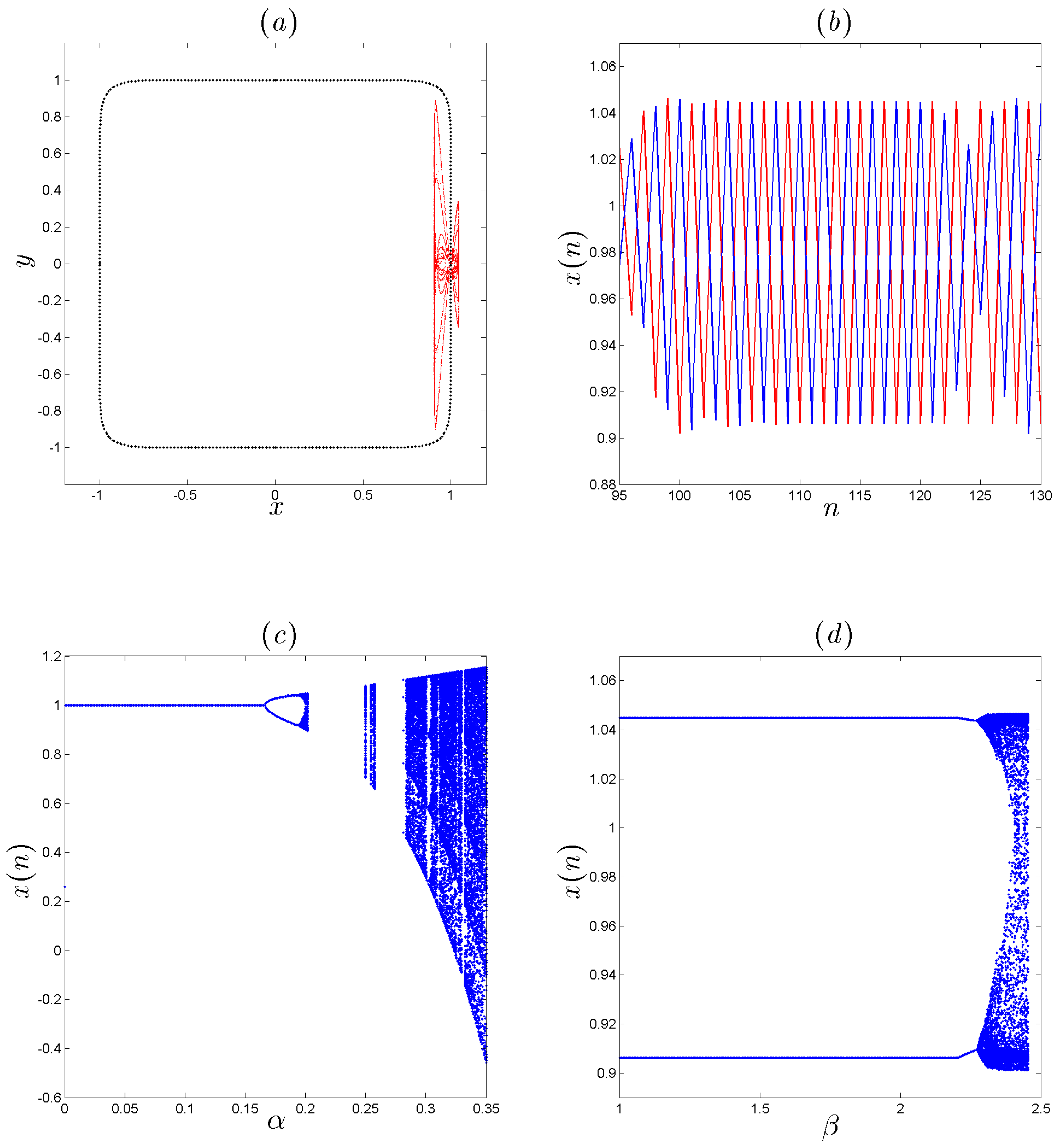
In this section, we will study the dynamical behavior of the novel fractional-order map (10) for some specific parameters and initial values. Figure 1 shows the chaotic attractor along with its bifurcation plots with respect to and , and the time evolution of states x for . The chaotic attractor of the fractional-order map (10) under system parameters and initial value is shown in Figure 1a, where the black points represent the square-shaped fixed points. Figure 1b gives the time evolutions of the variables x and y which illustrates that the system (10) has two symmetrical states. Figure 1c,d shows the bifurcation plots produced when fixing one of the parameters and varying the second. These bifurcation diagrams are constructed for 50 initial points. We see that the maximum chaotic range is observed for and . Also, we notice that the range of for which we obtain a chaotic behavior is very short. Hence, it is more interesting to visualize the effect of on the map’s dynamics.
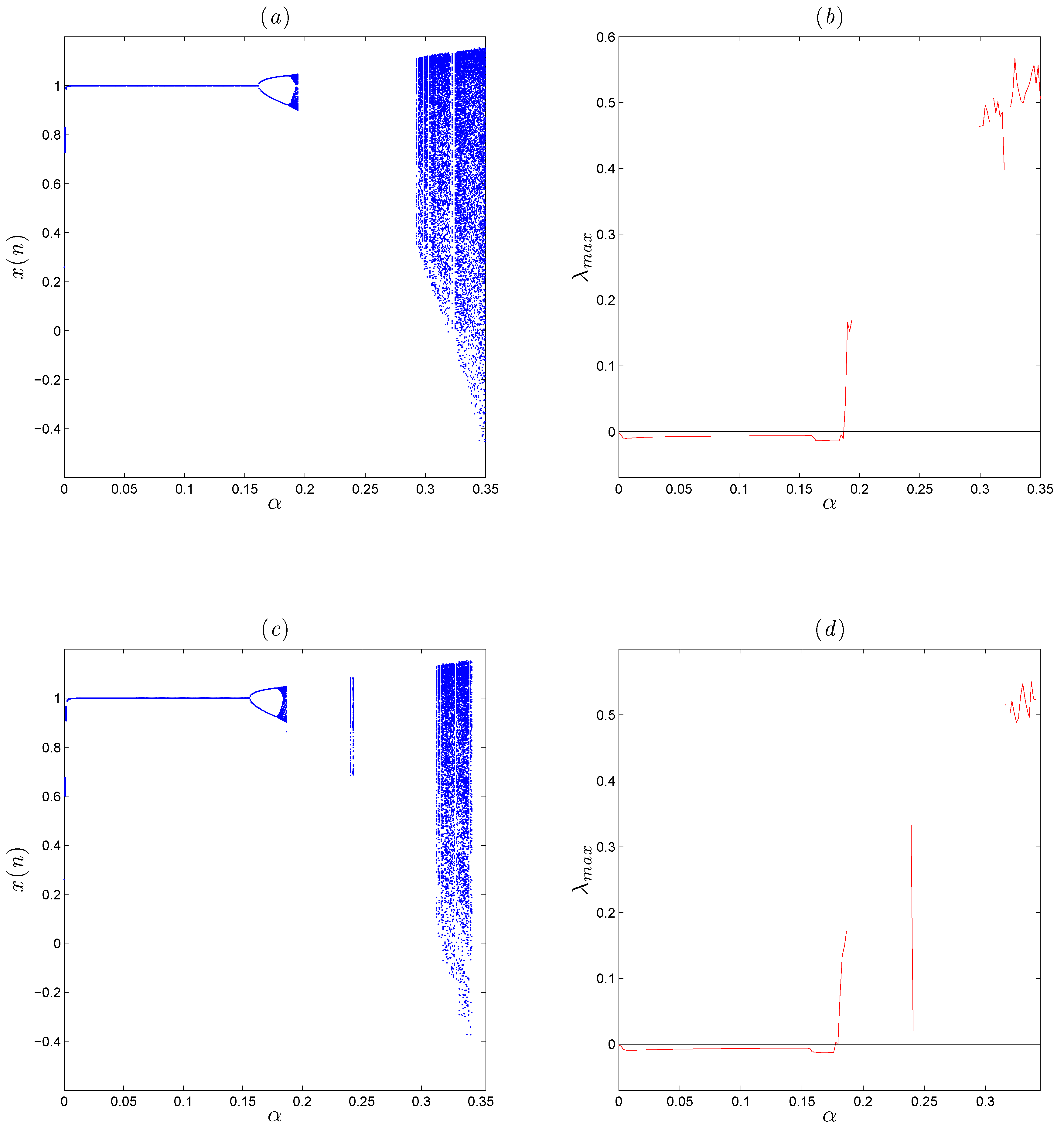
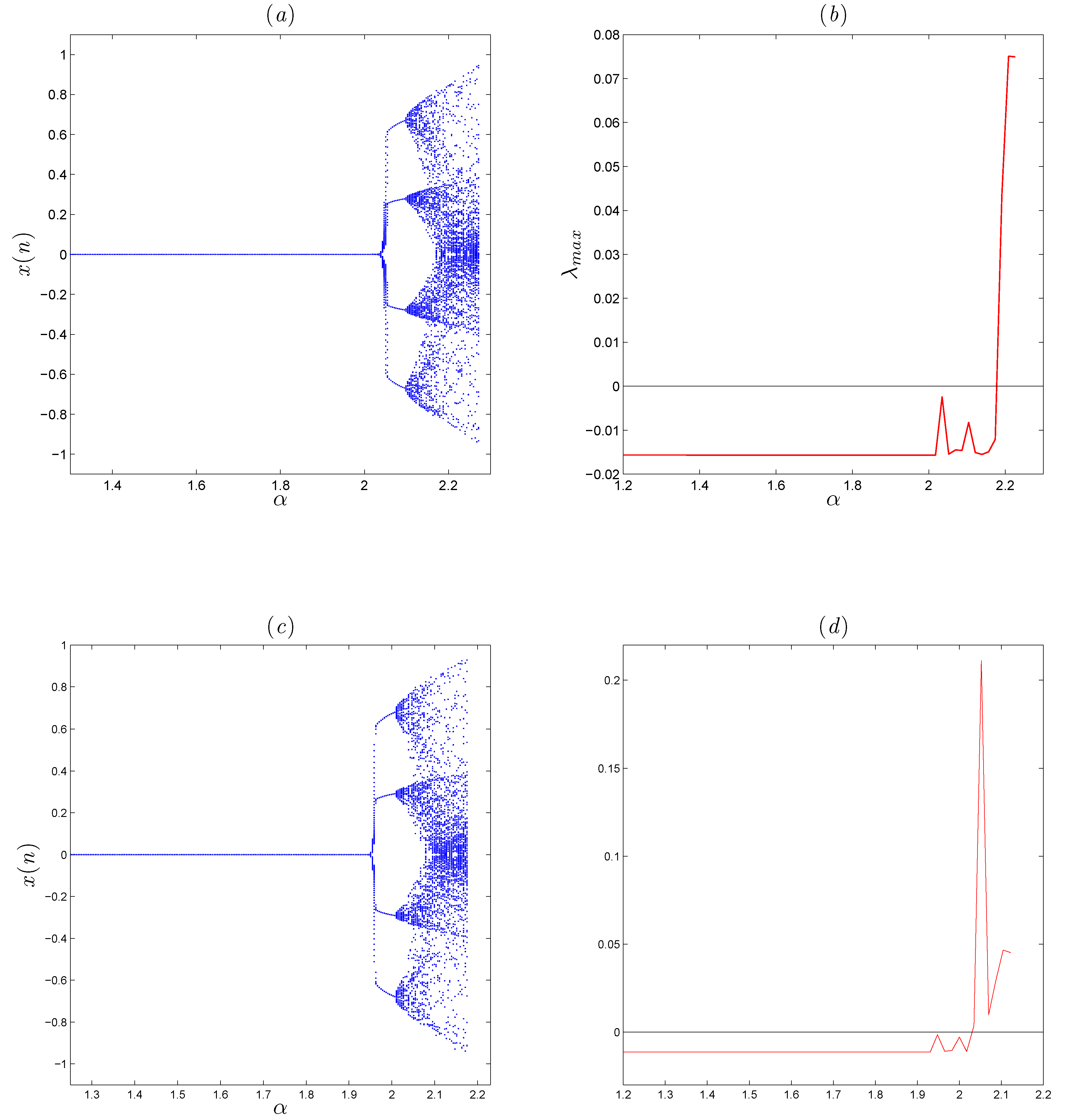
To investigate the sensitivity of the fractional-order map (10) with respect to the bifurcation parameter , we fix and we vary in the range The bifurcation diagrams and largest Lyapunov exponents under the fractional order and are given in Figure 2. By comparing Figure 2a,b with Figure 2c,d, we find that the interval where chaos exists shrinks as decreases. In particular, when the value of changes from to , the areas of chaotic motion shrinks from to . Also, the transient states region increases.
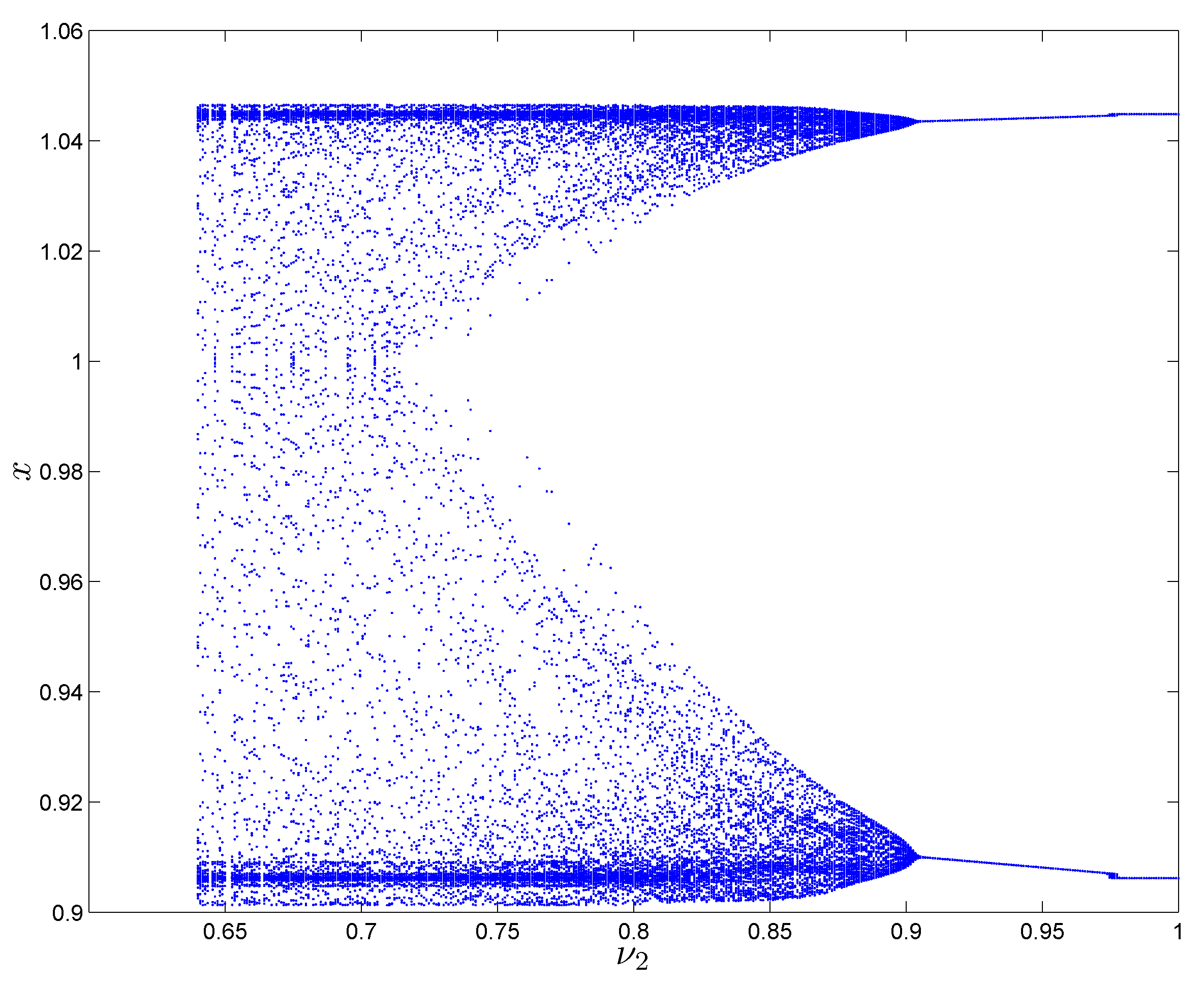
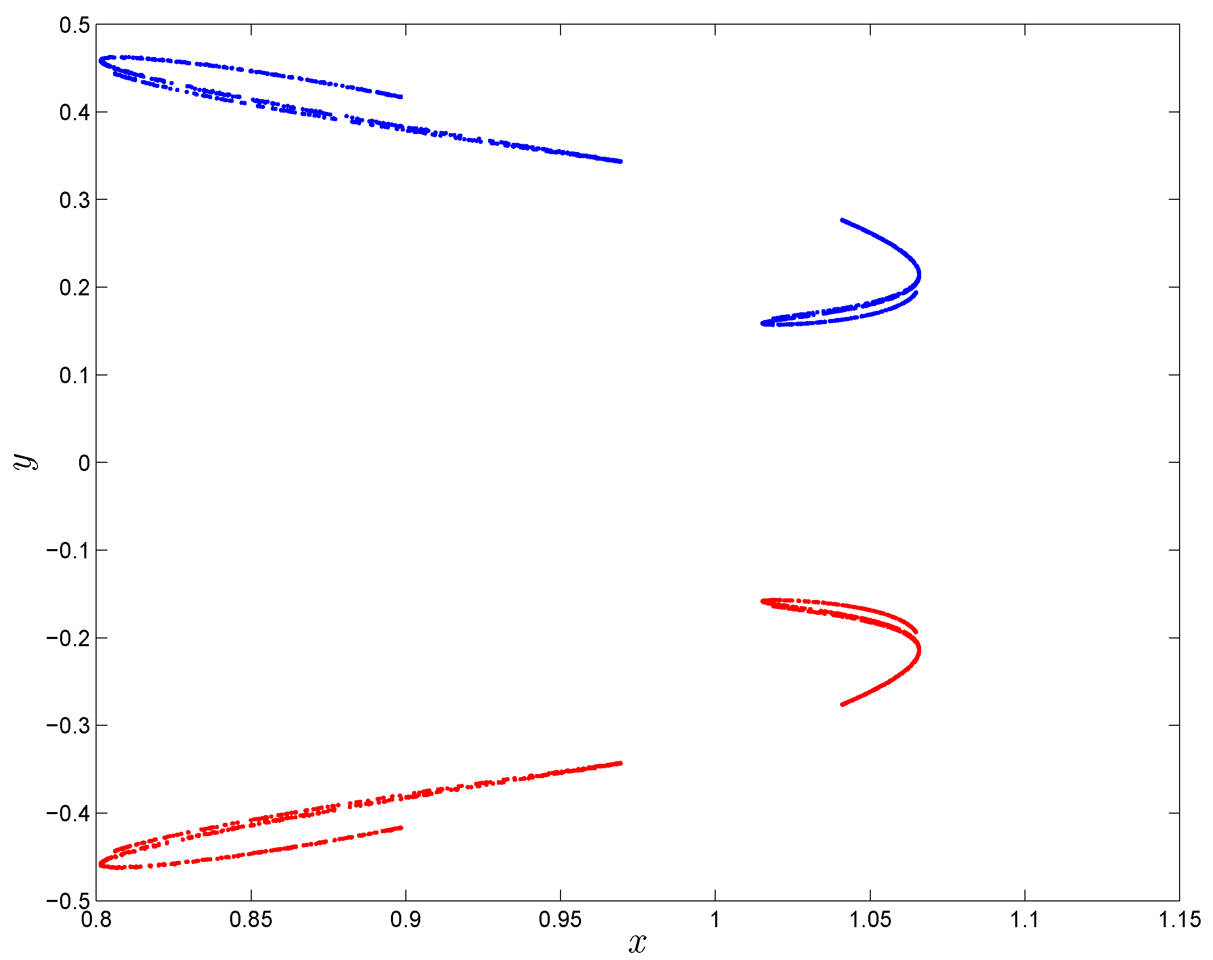
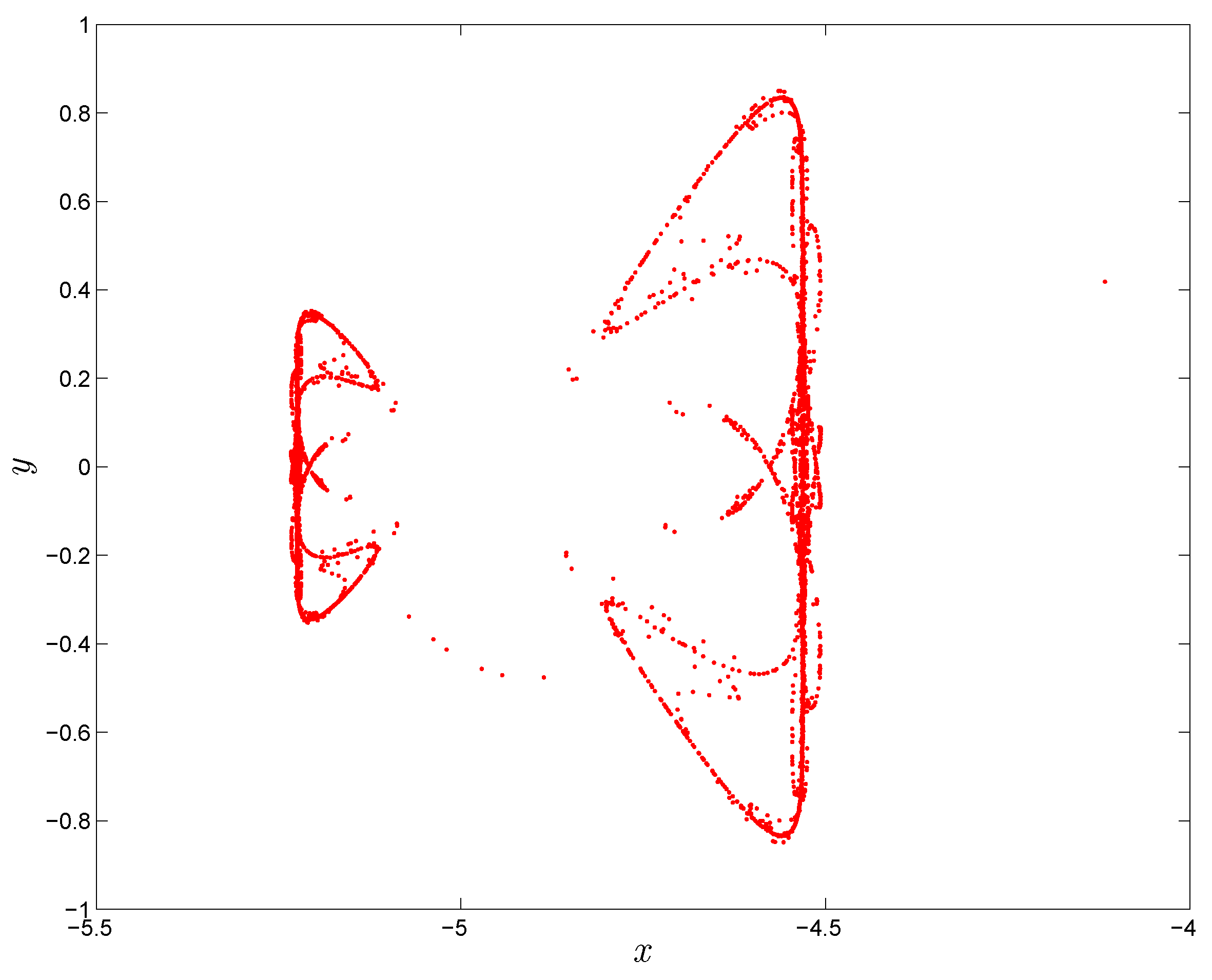
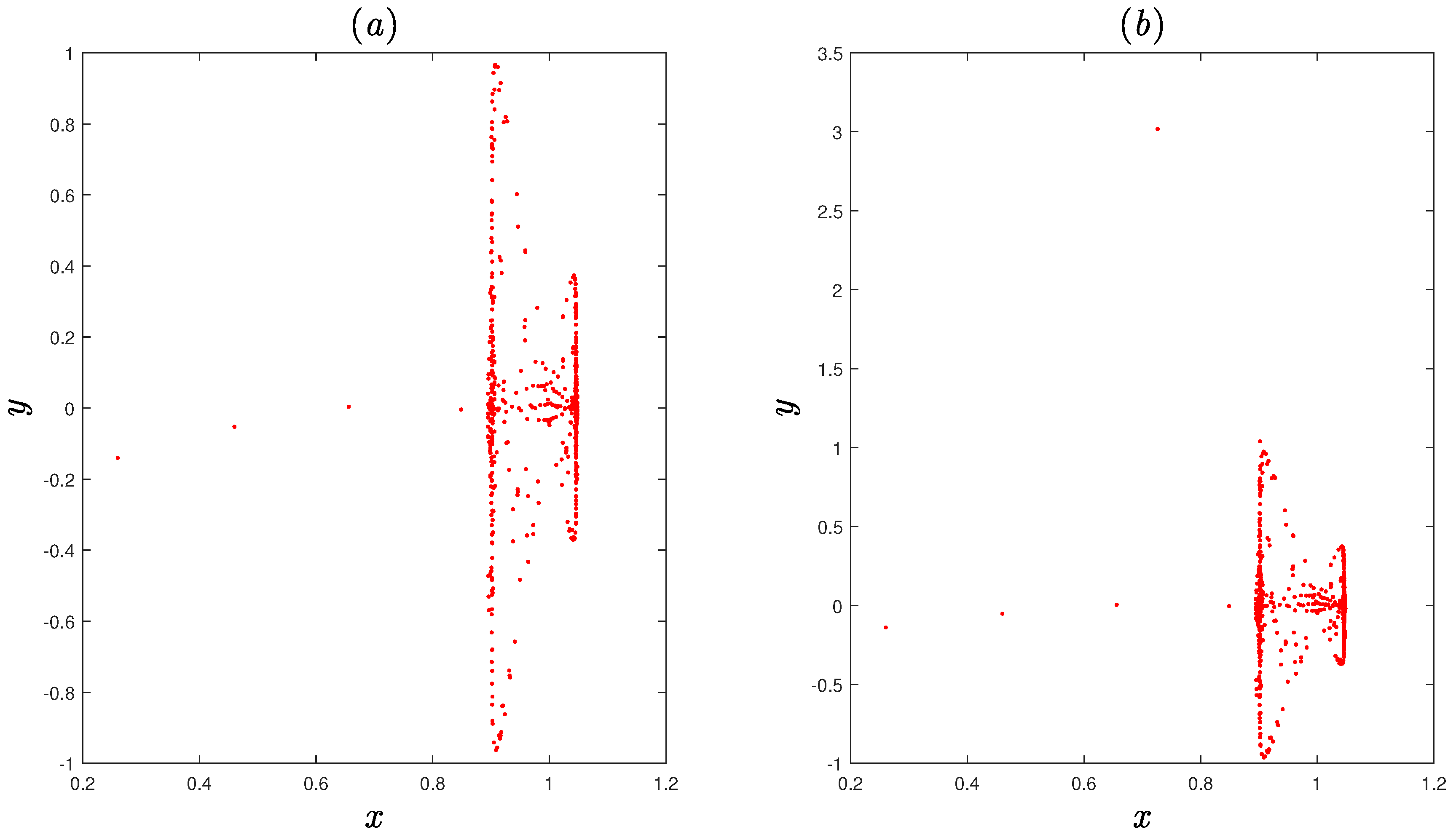
Now, reset the parameter and keep the parameter as Figure 3 shows the bifurcation diagram of the fractional-order map (10) with the decreasing of where . When decreases from 1, the fractional-order map (10) presents a periodic state until it enters into chaos at . It is noticed that the periodic state of the integer order map becomes chaotic as decreases. Another interesting dynamic is observed if we increase the value of to and decrease the value of to . In this case, two chaotic attractors are observed in the fractional-order map with respect to the fractional orders and , as shown in Figure 4, where the red color attractor is yielded from initial value and blue color attractor is yielded from initial value . Therefore, we conclude that the fractional order improves the complexity of the chaotic motion of the original system (7) with square-shaped fixed points.
3.2. A New Fractional Map with Rectangle-Shaped Fixed Points
Now, we consider system (7) when , , , . In this case we have the following system:
where x and y are the system variables. Using the same argument as with the previous system, we obtain the following fractional-order map:
where is the fractional order. The fixed points of the new fractional-order map (16) are obtained by solving the following system of equation:
Thus, we must have
Therefore, the novel fractional-order map (16) has rectangle-shaped fixed points.
To study the dynamic behavior of the novel fractional-order map (16), we define the numerical formula as:
where and are the initial conditions.
Bifurcation and Largest Lyapunov Exponents
In this section we investigate the dynamic behavior of the new fractional-order map (16) using numerical simulations. When the fractional-order map (16) shows the hidden chaotic attractor as depicted in Figure 5. It can be shown that it also has a symmetry with respect to the x-axis. Figure 6 shows the bifurcation diagrams and largest Lyapunov exponents of the fractional-order map (16). According to Figure 6, it is very clear that the dynamic behavior of system (16) goes from periodic state to chaotic state with the increase of the control parameter . Obviously, as the fractional order decreases from to , the bifurcation diagram gradually shrinks to the left.
3.3. 0–1 Test
In order to further confirm the influence of the fractional order on the properties of the fractional-order maps, we apply a new approach proposed by Gottwald and Melbourne called the 0–1 test method [25]. Unlike other methods, the test does not involve phase space reconstruction, and we can applied it directly to the series data The output is either 0 or 1 depending on whether the nature of the system is regular or chaotic. Naturally, we do not obtain the values 1 and 0 exactly, so the test remains valid when K is close enough to these values.
Here, we applied the 0–1 test method directly to the state that was obtained from the numerical formulas (14) and (19), respectively. For an arbitrary constant c in we calculate the translation variables
The dynamics of the translation components provide a visual test. Basically, if the dynamic is regular then the behavior of trajectories in the plane is bounded, whereas if the dynamic is chaotic then the trajectories depict Brownian like behavior. In order to examine the diffusive behavior of and , we define the mean square displacement as:
with the asymptotic growth rate of
In practice, the final result K can be determined numerically by computing the median of When 1, the behavior is classified as chaotic and when K is close to 0 the behavior is regular.
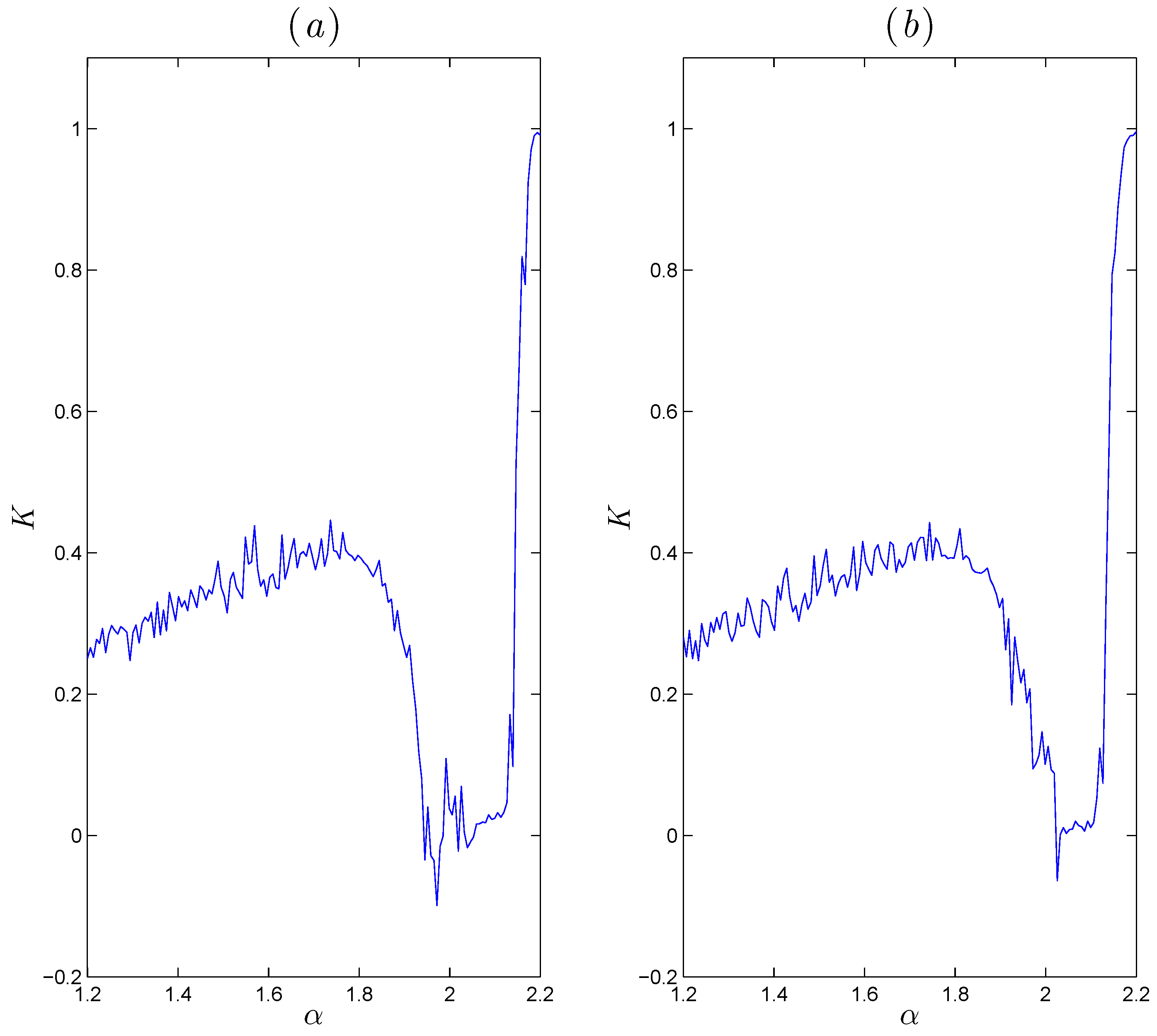
In Figure 7, we present the 0–1 test of the fractional-order map (10), when and . It is clear that the output K converges to the values 1, which implies that system (10) is chaotic. Moreover, when the fractional-order map (10) has a transient state as shown in Figure 8. As it can be seen that the state first converges into a bounded attractor and then it becomes divergent.
4. Conclusions
In this article, we investigated the chaotic behavior of new two-dimensional fractional chaotic maps with closed curve fixed points. Numerical methods, including computations of Lyapunov exponents, bifurcation diagrams, and the 0–1 test have been used to illustrate the complex dynamics of these systems. Through this paper, we have shown that chaos exists in these fractional-order maps and that the type and range of chaotic behavior is dependent on the fractional order. Results shows that the fractional-order maps are more complex then their integer order counterparts. Also, numerical experiments have shown that the system exhibits the property of coexisting attractors. Future studies will explore more dynamic behaviors of those systems, such as, control and synchronization.
Author Contributions
Conceptualization, A.O., F.H.; N.S., and A.-A.K.; Data curation, A.-A.K. and F.H.; A.O. Investigation, F.H., A.O., and N.S.; Methodology, A.O., F.H., Supervision, N.S., A.O., and G.G.; Validation, A.O. and N.S. All authors have read and agreed to the published version of the manuscript.
Acknowledgments
The author Adel Ouannas was supported by the Directorate General for Scientific Research and Technological Development of Algeria.
Conflicts of Interest
The authors declare no conflict of interest.
References
- Atıcı, F.M.; Eloe, P.W. Discrete fractional calculus with the nabla operator. Electron. J. Qual. Theory Differ. Equ. 2009, 1–12. [Google Scholar] [CrossRef]
- Abdeljawad, T.; Baleanu, D.; Jarad, F.; Agarwal, R.P. Fractional sums and differences with binomial coefficients. Discret. Dyn. Nat. Soc. 2013, 1–6. [Google Scholar] [CrossRef] [Green Version]
- Abdeljawad, T. On Riemann and Caputo fractional differences. Comput. Math. Appl. 2011, 62, 1602–1611. [Google Scholar] [CrossRef] [Green Version]
- Baleanu, D.; Wu, G.C.; Bai, Y.R.; Chen, F.L. Stability analysis of Caputo–like discrete fractional systems. Commun. Nonlinear Sci. Numer. Simul. 2017, 48, 520–530. [Google Scholar] [CrossRef]
- Goodrich, C.; Peterson, A.C. Discrete Fractional Calculus; Springer: Berlin, Germany, 2015; ISBN 978-3-319-79809-7. [Google Scholar]
- Ross, B. The development of fractional calculus 1695–1900. Hist. Math. 1977, 4, 75–89. [Google Scholar] [CrossRef] [Green Version]
- Kilbas, A.A.A.; Srivastava, H.M.; Trujillo, J.J. Theory and Applications of Fractional Differential Equations; Elsevier Science Limited: New York, NY, USA, 2006; Volume 204, ISBN 9780444518323. [Google Scholar]
- Miller, K.S.; Ross, B. Fractional Difference Calculus. In Proceedings of the International Symposium on Univalent Functions, Fractional Calculus and Their Applications, Nihon University, Koriyama, Japan, May 1988; Ellis Horwood Ser. Math. Appl.; Horwood: Chichester, UK, 1989; pp. 139–152. [Google Scholar]
- Atici, F.M.; Eloe, P.W. A transform method in discrete fractional calculus. Int. J. Differ. Equ. 2007, 2, 165–176. [Google Scholar]
- Atıcı, F.M.; Eloe, P.W. Two-point boundary value problems for finite fractional difference equations. J. Differ. Equ. App. 2011, 17, 445–456. [Google Scholar] [CrossRef]
- Atici, F.; Eloe, P. Initial value problems in discrete fractional calculus. Am. Math. Soc. 2009, 137, 981–989. [Google Scholar] [CrossRef]
- Wu, G.C.; Baleanu, D. Discrete fractional logistic map and its chaos. Nonlinear Dyn. 2014, 75, 283–287. [Google Scholar] [CrossRef]
- Wu, G.C.; Baleanu, D.; Zeng, S.D. Discrete chaos in fractional sine and standard maps. Phys. Lett. A 2014, 378, 484–487. [Google Scholar] [CrossRef]
- Wu, G.C.; Baleanu, D.; Huang, L.L. Novel Mittag-Leffler stability of linear fractional delay difference equations with impulse. Appl. Math. Lett. 2018, 82, 71–78. [Google Scholar] [CrossRef]
- Strogatz, S.H. Nonlinear Dynamics and Chaos: With Applications to Physics, Biology, Chemistry, and Engineering, 2nd ed.; Westview Press: Boulder, CO, USA, 2015; ISBN 978-0813349107. [Google Scholar]
- Uchida, A. Optical Communication with Chaotic Lasers: Applications of Nonlinear Dynamics and Synchronization, 1st ed.; John Wiley & Sons: Weinheim, Germany, 2012; ISBN 9783527408696. [Google Scholar]
- Guegan, D. Chaos in economics and finance. Annu. Rev. Control. 2009, 33, 89–93. [Google Scholar] [CrossRef] [Green Version]
- Ugarcovici, I.; Weiss, H. Chaotic dynamics of a nonlinear density dependent population model. Nonlinearity 2004, 17, 1689–1711. [Google Scholar] [CrossRef] [Green Version]
- Sengul, S. Discrete Fractional Calculus and Its Applications to Tumor Growth. Master’s Theses, Western Kentucky University, Bowling Green, KY, USA, 1 May 2010; p. 161. [Google Scholar]
- Akin, E.; Kolyada, S. Li-Yorke sensitivity. Nonlinearity 2003, 16, 1421–1433. [Google Scholar] [CrossRef]
- Liu, Y. Chaotic synchronization between linearly coupled discrete fractional Hénon maps. Indian J. Phys. 2010, 90, 313–317. [Google Scholar] [CrossRef]
- Lozi, R. Un attracteur étrange du type attracteur de Hénon. Le Journal de Physique Colloques 1978, 39, C5–C9. [Google Scholar] [CrossRef]
- Shukla, M.K.; Sharma, B.B. Investigation of chaos in fractional order generalized hyperchaotic Henon map. Aeu-Int. J. Electron. C 2017, 78, 265–273. [Google Scholar] [CrossRef]
- Li, C.; Chen, Y.; Kurths, J. Fractional calculus and its applications. Philos. Tr. Soc. A 2013, 371, 20130037. [Google Scholar] [CrossRef] [Green Version]
- Gottwald, G.A.; Melbourne, I. The 0-1 test for chaos: A review. In Chaos Detection and Predictability; Springer: Berlin/Heidelberg, Germany, 2016; pp. 221–247. [Google Scholar] [CrossRef]
- Ouannas, A.; Khennaoui, A.A.; Zehrour, O.; Bendoukha, S.; Grassi, G.; Pham, V.T. Synchronisation of integer-order and fractional-order discrete-time chaotic systems. Pramana 2019, 92, 52. [Google Scholar] [CrossRef]
- Ouannas, A.; Wang, X.; Khennaoui, A.A.; Bendoukha, S.; Pham, V.T.; Alsaadi, F. Fractional form of a chaotic map without fixed points: Chaos, entropy and control. Entropy 2018, 20, 720. [Google Scholar] [CrossRef] [Green Version]
- Elaydi, S.N. Discrete Chaos: With Applications in Science and Engineering; Chapman and Hall/CRC: New York, NY, USA, 2007; ISBN 9780429149191. [Google Scholar]
- Khennaoui, A.A.; Ouannas, A.; Bendoukha, S.; Grassi, G.; Wang, X.; Pham, V.T.; Alsaadi, F.E. Chaos, control, and synchronization in some fractional-order difference equations. Adv. Differ. Equ. 2019, 2019, 1–23. [Google Scholar] [CrossRef] [Green Version]
- Ouannas, A.; Khennaoui, A.A.; Bendoukha, S.; Grassi, G. On the Dynamics and Control of a Fractional Form of the Discrete Double Scroll. Int. J. Bifurc. Chaos. 2019, 29, 1950078. [Google Scholar] [CrossRef]
- Ouannas, A.; Khennaoui, A.A.; Odibat, Z.; Pham, V.T.; Grassi, G. On the dynamics, control and synchronization of fractional-order Ikeda map. Chaos Soliton. Fract. 2019, 123, 108–115. [Google Scholar] [CrossRef]
- Ouannas, A.; Khennaoui, A.A.; Grassi, G.; Bendoukha, S. On chaos in the fractional-order Grassi–Miller map and its control. J. Comput. Appl. Math. 2019, 358, 293–305. [Google Scholar] [CrossRef]
- Jouini, L.; Ouannas, A.; Khennaoui, A.A.; Wang, X.; Grassi, G.; Pham, V.T. The fractional form of a new three-dimensional generalized Hénon map. Adv. Differ. Equ. 2019, 2019, 122. [Google Scholar] [CrossRef]
- Ouannas, A.; Khennaoui, A.A.; Bendoukha, S.; Vo, T.; Pham, V.T.; Huynh, V. The fractional form of the Tinkerbell map is chaotic. Appl. Sci. 2018, 8, 2640. [Google Scholar] [CrossRef] [Green Version]
- Wu, G.C.; Baleanu, D. Discrete chaos in fractional delayed logistic maps. Nonlinear Dynam. 2015, 80, 1697–1703. [Google Scholar] [CrossRef]
- Jiang, H.; Liu, Y.; Wei, Z.; Zhang, L. A New Class of Two-dimensional Chaotic Maps with Closed Curve Fixed Points. Int. J. Bifurc. Chaos 2019, 29, 1950094. [Google Scholar] [CrossRef]
Figure 1.
Numerical analysis of the fractional-order map (10) for . (a) Square-shaped fixed point of the fractional-order map are illustrated with black dots and the hidden chaotic attractor in red. (b) Evolution states of the fractional-order map (10) of x and y. (c) Bifurcation diagram of the fractional-order map (10) versus for . (d) Bifurcation diagram of the fractional-order map (10) versus for .

Figure 2.
(a) Bifurcation diagram of the fractional-order map (10) versus for . (b) Largest Lyapunov exponents corresponding to (a). (c) Bifurcation diagram of the fractional-order map (10) versus for . (d) Largest Lyapunov exponents corresponding to (c).

Figure 3.
Bifurcation diagram for system (10) in the plane for and .
Figure 3.
Bifurcation diagram for system (10) in the plane for and .

Figure 4.
Coexisting chaotic attractor of the fractional-order map (16) for and .
Figure 4.
Coexisting chaotic attractor of the fractional-order map (16) for and .

Figure 5.
Chaotic attractor of the fractional-order map (16) for .
Figure 5.
Chaotic attractor of the fractional-order map (16) for .

Figure 6.
(a) Bifurcation diagram of the fractional-order map (16) versus for . (b) Largest Lyapunov exponents corresponding to (a). (c) Bifurcation diagram of the fractional-order map (16) versus for . (d) Largest Lyapunov exponents corresponding to (c).

Figure 7.
The 0–1 test method of the fractional-order map (10).
Figure 7.
The 0–1 test method of the fractional-order map (10).

Figure 8.
Transient state of the fractional-order map for (a) when , (b) when .

Figure 9.
The 0–1 test of the fractional-order map (16). (a) The asymptotic growth rate versus for . (b) The asymptotic growth rate versus for .
Figure 9.
The 0–1 test of the fractional-order map (16). (a) The asymptotic growth rate versus for . (b) The asymptotic growth rate versus for .

© 2020 by the authors. Licensee MDPI, Basel, Switzerland. This article is an open access article distributed under the terms and conditions of the Creative Commons Attribution (CC BY) license (http://creativecommons.org/licenses/by/4.0/).
Share and Cite
MDPI and ACS Style
Hadjabi, F.; Ouannas, A.; Shawagfeh, N.; Khennaoui, A.-A.; Grassi, G. On Two-Dimensional Fractional Chaotic Maps with Symmetries. Symmetry 2020, 12, 756. https://0-doi-org.brum.beds.ac.uk/10.3390/sym12050756
AMA Style
Hadjabi F, Ouannas A, Shawagfeh N, Khennaoui A-A, Grassi G. On Two-Dimensional Fractional Chaotic Maps with Symmetries. Symmetry. 2020; 12(5):756. https://0-doi-org.brum.beds.ac.uk/10.3390/sym12050756
Chicago/Turabian StyleHadjabi, Fatima, Adel Ouannas, Nabil Shawagfeh, Amina-Aicha Khennaoui, and Giuseppe Grassi. 2020. "On Two-Dimensional Fractional Chaotic Maps with Symmetries" Symmetry 12, no. 5: 756. https://0-doi-org.brum.beds.ac.uk/10.3390/sym12050756
Note that from the first issue of 2016, this journal uses article numbers instead of page numbers. See further details here.