Article

Persistence Analysis and Prediction of Low-Visibility Events at Valladolid Airport, Spain

by
Sara Cornejo-Bueno
1,2,
David Casillas-Pérez
1,2,
Laura Cornejo-Bueno
2,
Mihaela I. Chidean
2,
Antonio J. Caamaño
2,
Julia Sanz-Justo
3,
Carlos Casanova-Mateo
3 and
Sancho Salcedo-Sanz
1,*
1
Department of Signal Processing and Communications, Universidad de Alcalá, 28805 Alcalá de Henares, Spain
2
Department of Signal Processing and Communications, Universidad Rey Juan Carlos, 28943 Fuenlabrada, Spain
3
LATUV, Remote Sensing Laboratory, Universidad de Valladolid, 47011 Valladolid, Spain
*
Author to whom correspondence should be addressed.
Submission received: 19 May 2020 / Revised: 19 June 2020 / Accepted: 21 June 2020 / Published: 23 June 2020

Abstract

:
This work presents an analysis of low-visibility event persistence and prediction at Villanubla Airport (Valladolid, Spain), considering Runway Visual Range (RVR) time series in winter. The analysis covers long- and short-term persistence and prediction of the series, with different approaches. In the case of long-term analysis, a Detrended Fluctuation Analysis (DFA) approach is applied in order to estimate large-scale RVR time series similarities. The short-term persistence analysis of low-visibility events is evaluated by means of a Markov chain analysis of the binary time series associated with low-visibility events. We finally discuss an hourly short-term prediction of low-visibility events, using different approaches, some of them coming from the persistence analysis through Markov chain models, and others based on Machine Learning (ML) techniques. We show that a Mixture of Experts approach involving persistence-based methods and Machine Learning techniques provides the best results in this prediction problem.

1. Introduction

Very low-visibility events due to fog are classified among severe weather conditions that most affect air traffic and flight operations at airports [1,2,3], since they can dramatically reduce the runway capacity [4]. In foggy conditions, airport managers activate specific low-visibility procedures to sustain safe operations. In fact, in extreme situations, the reduced visibility can cause the suspension of the runway operations, or even the temporary closure of the complete airport. Forecasting low-visibility conditions is therefore a recurrent problem for airport managers. It is, however, a very difficult task requiring both knowledge of the meteorological causes of fog formation, and a thorough awareness of the local topography.
Very different techniques have been developed to help forecasters improve the prediction of reduced-visibility events at airports facilities. Numerical weather prediction is one of the most widely-used approaches. However, as stated by many authors [5,6,7,8], the forecasting of fog events by numerical weather prediction is particularly difficult, in part because fog formation is extremely sensitive to small-scale variations of atmospheric variables, such as wind-shifts or changes in the low-level stability. Other approaches consist of using statistical methods for predicting low-visibility events. One of the first attempts was the use of linear regression [9], but the recent development of Machine Learning (ML) has produced high-quality algorithms for the prediction of low-visibility events, based on non-linear approaches such as artificial neural networks, fuzzy logic, Bayesian networks or support vector machines [10,11,12,13,14,15,16,17].
In spite of this huge work on different prediction techniques, there are some aspects related to low-visibility events which have not been exploited enough in the developing of new forecasting algorithms. One of them is, without doubt, the fact that low-visibility events due to fog are highly persistent phenomena. The persistence of these events is a well known fact, but very little work on exploiting this fact in prediction systems can be found in the literature [18]. Persistence analysis of other atmospheric and oceanic phenomena has been frequent [19,20], with recent studies taking into account rainfall and hydrology [21,22], wind [23,24,25], sea surface temperature [26] or solar radiation [27,28] time series, but not for fog or mist events.
In this paper we carry out a complete study of persistence in low-visibility events due to fog at Villanubla Airport (Valladolid, Spain). This area is well-known for persistent radiation fog episodes in winter, which sometimes compromise the airport activity. Our analysis takes into account long-term and short-term fog persistence, and its short-term prediction, using different techniques such as Detrended Fluctuation Analysis (DFA), Markov Chain Models (MCMs) analysis and ML algorithms. After the persistence analysis, we will show how prediction methods based on persistence are extremely efficient for very short-term prediction of fog events. This prediction problem has been tackled in this paper as a binary classification task that is highly unbalanced (there are much more samples of the class “no-fog” than of the class “low-visibility event” (fog)). We have then designed a high quality approach for low-visibility events prediction based on a Mixture of Experts (MOE), which includes the Naïve persistence operator, and several ML algorithms with a procedure to balance the dataset.
The remainder of the paper is structured in the following way: the next section presents the available data at Villanubla Airport, and the description of the methods considered for this analysis. Section 3 shows the results on persistence in low-visibility events carried out both in long-term and short-term time horizons. Section 4 discusses the main results obtained in this research, and closes the paper with some concluding remarks about this work. Finally, note that we have included a list of acronyms at the end of the manuscript to make easier its reading.

2. Data and Methods

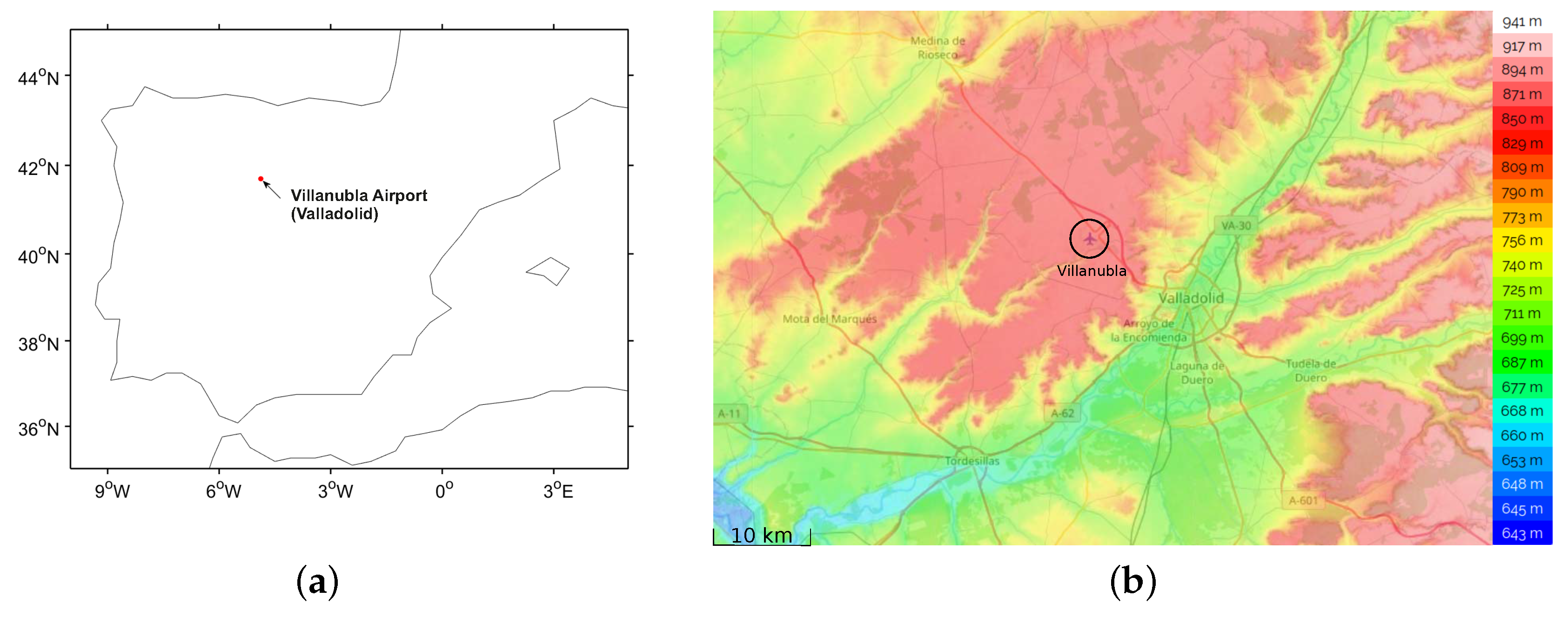
2.1. Data Description

We consider the prediction of low-visibility events at Villanubla Airport, Spain (41.70 N, 4.88 W), see Figure 1. This area is well-known for its low-visibility episodes, with the radiation fog as the most frequent fog phenomenon [7], due to the geographical and climatological characteristics of the zone. This zone is located in a valley surrounded by hills (“Montes Torozos”), and near the Duero river basin [29]. These two conditions, together with the low winter temperatures observed in the area, are good ingredients for the formation of radiation fog in winter [30]. The target variable to analyze low-visibility events is the Runway Visual Range (RVR) of the airport, obtained from three visibilimeters deployed along the airport runway (the touchdown zone, the mid-point and stop-end of the runway), which belong to the aeronautical observation network of the Meteorological State Agency of Spain. These instruments are managed under a quality-management system certified by ISO 9001:2008, which guarantees measurement accuracy, and ensures the international standards compliance of the measurements.
We consider hourly RVR data at Villanubla airport from years 2008 to 2013 during the months when radiation fog is most intense according to [30] (November, December, January and February). To study the occurrence of reduced-visibility conditions, we also use in some cases data from a 100-m meteorological tower at the Research Centre for the Lower Atmosphere (CIBA), which is located about 13 km north-north-west from the airport. Specifically, these exogenous variables are used as inputs in the ML techniques applied, in order to take into account the atmospheric state. The exogenous variables provide relevant atmospheric-state information to predict radiation fog, such as temperature, wind speed, atmospheric pressure or relative humidity in the zone. The complete list of exogenous and target variables considered in this paper are summarized in Table 1. We have employed four previous time steps (time windows for input variables) to take into account these predictive variables ( t 1 , t 2 , t 3 and t 4 ), in an attempt to obtain better results in the prediction than the Naïve persistence operator described later on. Finally, note that since the RVR time series is highly unbalanced (2027 fog events versus 11,261 no-fog events) we have applied an over-sampling technique, SMOTE (Synthetic Minority Over-sampling Technique), as will be further explained in Section 2.4.3.

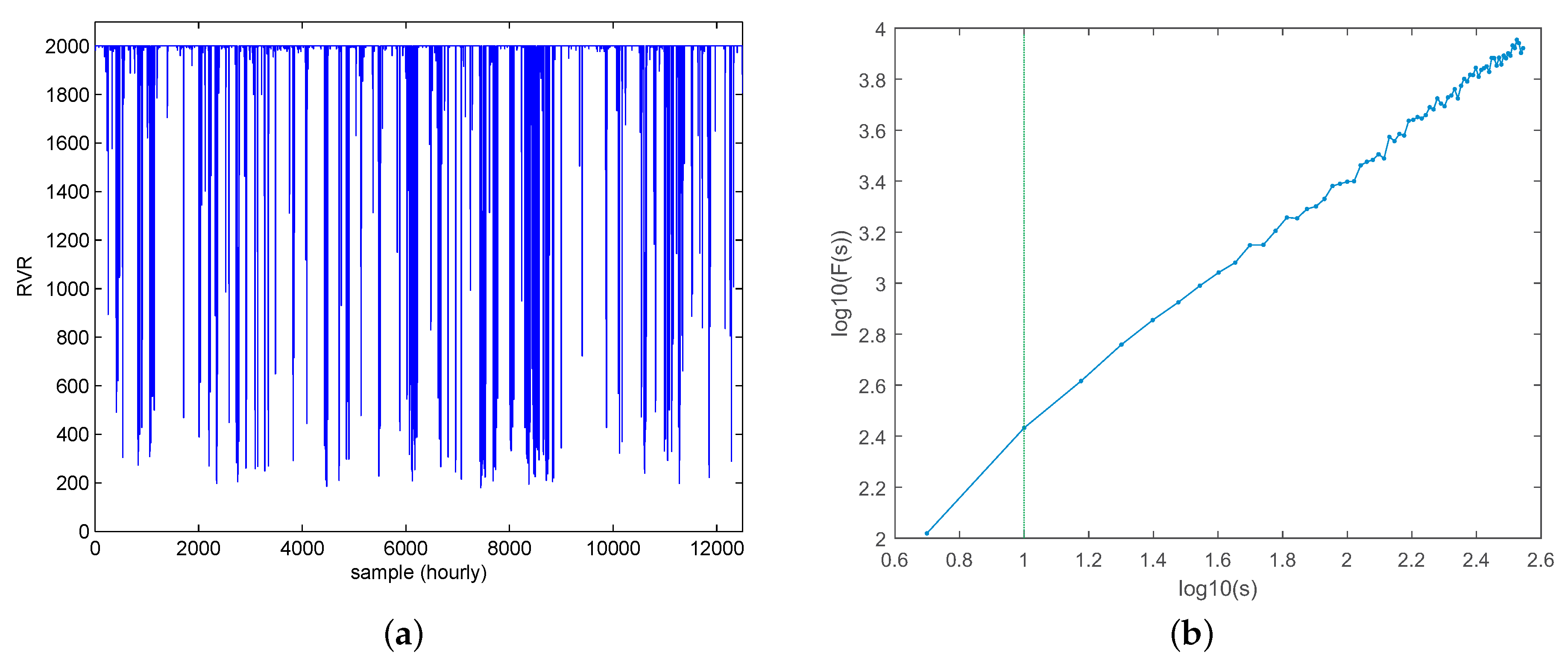
2.2. Methods for Long-Term Persistence: Detrended Fluctuation Analysis.

The DFA algorithm was first proposed by Peng et al., in two seminal papers [31,32]. Since then, it has been frequently used to analyze long-term persistence of time series in different applications [22,33]. The DFA algorithm consists of three main steps [34]:
(1)
We first remove the periodic annual cycle of the time series, by the procedure explained in detail in [22]. Adapted to our problem, the process consists of standardizing the input time series x i of length N as follows:
x i = x i x ¯ i σ i ,
where x i stands for the original hourly RVR time series, x ¯ i represents the mean value of the hourly RVR time series and σ i is its standard deviation.
(2)
Then, the time series profile Y j is computed as follows:
Y j = i = 1 j x i .
The profile Y j is divided into N s = N s non-overlapping segments { Y j k | 1 k N s } of equal length s.
For each segment Y j k , we calculate the local least squares straight-line Z j k which measures its local trend. As a result, we obtain a linear piece-wise function Z ˜ j s compounding each linear fitting:
Z ˜ j s = Z j 1 Z j k Z j N s ,
where the superscript s refers to the time window length used to the linear fitting of each piece.
(3)
We then obtain the so-called fluctuation as the root-mean-square error from this linear piece-wise function Z ˜ j s and the profile Y j , varying the time window length s:
F ( s ) = 1 N k = 1 N ( Z ˜ j s Y j ) 2
At the time scale range where the scaling holds, F ( s ) increases with the time window s following a power law F ( s ) s α . Thus, the fluctuation F ( s ) versus the time scale s would be depicted as a straight line in a log-log plot. The slope of the fitted linear regression line is the scaling exponent α , also called correlation exponent. The scaling exponent α in the DFA method is a generalization of the Hurst exponent (H) [35], and in this context they have the same meaning. The Hurst coefficient is frequently used as a measure of long-term persistence of time series, i.e., H (or α in our case) provides a measure of possible simple power law scaling of the power spectrum S ( f ) with frequency f (sometimes referred to as “self-similar” behavior [36]):
S ( f ) f β
where the scaling exponent β is given by β = 2 α 1 .
Note that when the coefficient α = 0 . 5 , the time series is uncorrelated, which means that there is no long-term persistence in the time series. For larger values of α ( 0 . 5 < α 1 ), the time series is positively long-term correlated, which also means the long-term persistence exists across the corresponding scale range. When 0 < α 0 . 5 the process is anti-persistent. For α > 1 , the persistence becomes so extreme that the time series exhibits non-stationary behavior.

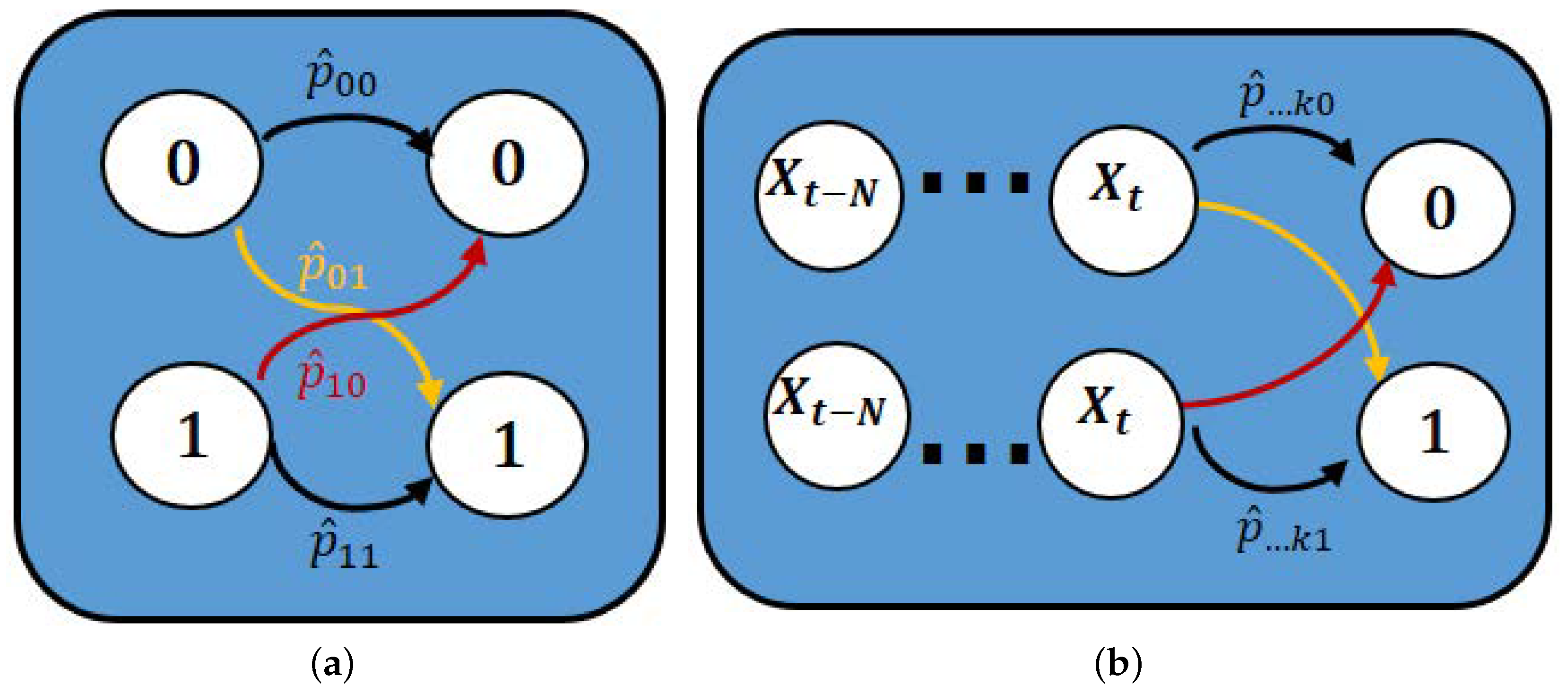
2.3. Methods for Short-Term Persistence: Markov Chain Models

Many statistical methods have been used for meteorological forecasting [37]. One of the statistical techniques employed in short-term prediction of meteorological time series are MCMs. The great advantage of using MCMs is its low computational cost, in addition to the possibility of doing an immediate forecasting after the observations, because they use local information of the meteorological variables [38]. We can find some chain-dependent processes in meteorology (e.g., temperature, precipitation amount, etc.) which can be explained in terms of an underlying first-order Markov chain [39].
In the present case of low-visibility events, we can consider a discrete binary variable with two possible states. That is, the RVR time series, converted to a binary variable, can take value 1, which means fog (low-visibility event), or 0, which means no-fog. Consequently, assuming that the occurrence probability of fog at present time depends on the previous hour state (first-order Markov chain), the transition probabilities of hourly fog can be divided into the following four cases:
p 00 = P X t = 0 | X t 1 = 0 p 01 = P X t = 1 | X t 1 = 0 p 10 = P X t = 0 | X t 1 = 1 p 11 = P X t = 1 | X t 1 = 1 .
An explanatory diagram is represented in Figure 2 for a first-order and N-order MCM.
We estimate the transition probabilities through the conditional relative frequencies, as follows:
p ^ 00 = n 00 n 0 p ^ 01 = n 01 n 0 p ^ 10 = n 10 n 1 p ^ 11 = n 11 n 1 ,
where n i j represents the number of transitions from state i to state j, and n i is the number of states i followed by any other data point, i.e., n i = n i 0 + n i 1 . The subscripts refer to the state, i , j { 0 , 1 } . Note that the Naïve persistence operator is a special case of first-order Markov chain, whose formula x ( t + 1 ) = x ( t ) forces the state preservation at any time, and it can also be described with the following transition probability matrix:
P = 1 0 0 1 .
For a higher-order MCM, the transition probabilities take into account the states at the time windows considered. The memoryless property characteristic of the first-order Markov chain breaks for the higher-order chains. For example, in a second-order Markov chain, the states at times t 2 and t 1 are considered to predict the state t; or in a third-order Markov chain, the states at times t 3 , t 2 and t 1 are taken into account to predict the state t. The transition probabilities for second and third-order respectively are defined as:
p i 2 i 1 i = P X t = i | X t 1 = i 1 , X t 2 = i 2 , i , i 1 , i 2 { 0 , 1 }
p i 3 i 2 i 1 i = P X t = i | X t 1 = i 1 , X t 2 = i 2 , X t 3 = i 3 , i , i 1 , i 2 , i 3 { 0 , 1 }
and so on for higher-orders:
p α i = P X t = i | X t 1 = α 1 , , X t N = α N , i { 0 , 1 } , α = ( α 1 , , α N ) { 0 , 1 } N ,
where α is a tuple of N elements which encompass all time windows considered.

2.4. Machine Learning Techniques for Classification and Prediction

Two state-of-the-art ML classification algorithms are considered in this work to solve the prediction of low-visibility events at Valladolid airport: Support Vector Machines (SVMs) [40,41], and Extreme Learning Machines (ELMs) [42,43]. The SVM is a well-established statistical learning technique, based on kernels. The ELM is a very fast-training algorithm, since it is based on a pseudo-inverse calculation. Note that both algorithms are focused on solving classification problems [44], i.e., in this paper we tackle the low-visibility prediction as a classification task.

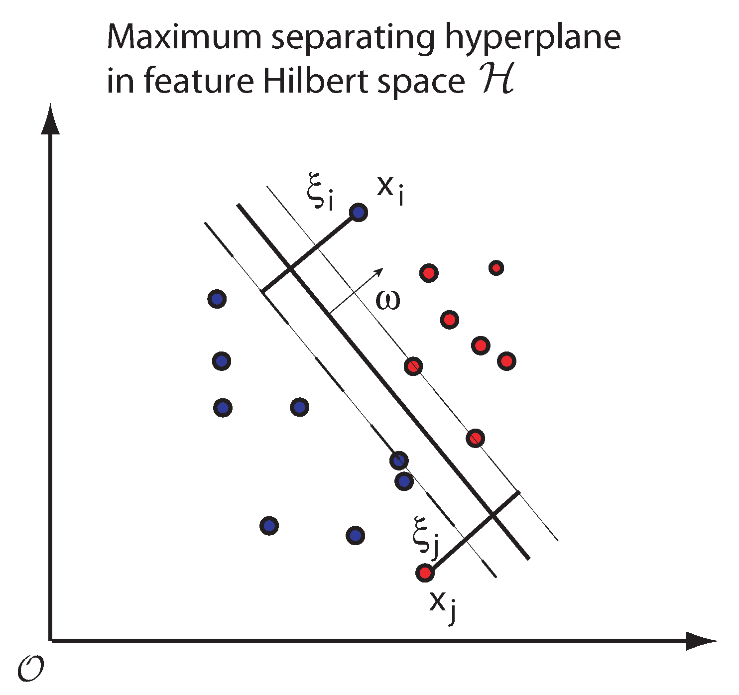
2.4.1. Support Vector Machines

The formulation of the standard SVM is defined as a maximum margin classifier, that is, a classifier whose decision function is a hyperplane that maximally separates samples from different classes (in this paper class 1 is understood to be a “low-visibility” state, and class −1 (equivalent to 0) stands for “no-fog” state). Given a labeled training data set { ( x i , y i ) } i = 1 n , where x i R N and y i { 1 , + 1 } , and given a non-linear mapping ϕ ( · ) : R N R p ( N p ), the SVM method solves:
min w , b , ξ 1 2 w + C i = 1 N ξ i s . t . y i w , ϕ ( x i ) + b + ξ i 1 0 i = 1 , , n ξ i 0 i = 1 , , n ,
where w and b define a separating hyperplane in R N and ξ i are positive slack variables enabling to deal with permitted errors, see Figure 3.
Note that the objective function of the problem Equation (12) is composed of two terms with a clear interpretation: one term tries to minimize the committed errors, i = 1 n ξ i , while the other one minimizes the Euclidean norm of the model weights, w 2 , which can be shown to be equivalent to the maximization of the margin (separation between classes). Note that one could just maximize the margin without including the errors in the objective function, driving to the so-called hard margin SVM. By including the slack variables ξ i , it is possible to relax the problem, managing non-separable data and yielding to the so-called soft margin SVM, which minimizes the training error traded off against the margin.
An appropriate choice of the non-linear mapping ϕ : R N R p guarantees that the transformed samples are more likely to be linearly separable in the higher-dimension feature space R p ( N p ). The regularization hyperparameter C controls the generalization capability of the classifier, and it must be usually tuned by the user. The primal problem giving by Equation (12) is solved by its dual problem counterpart [45] driving to the following decision function for any test sample x * R N :
f ( x * ) = s g n i = 1 n y i α i K ( x i , x * ) + b ,
where α i are the Lagrange multipliers corresponding to the constraints of the primal problem (12). The so-called support vectors (SVs) are those training samples x i with a corresponding non-zero Lagrange multiplier α i 0 . The function K ( x i , x * ) is the scalar product of the high-order space R p mapped from the sample space. It projects any test sample x * into the support vectors x i mapped to the higher-dimensional space. Finally, the bias term b is calculated using any of the constraints corresponding to an unbounded Lagrange multiplier as:
b = 1 k i = 1 k y i ϕ ( x i ) , w ,
where k is the number of unbounded Lagrange multipliers (i.e., 0 < α i < C ) and w = i = 1 n y i α i ϕ ( x i ) [45]. The specific SVM functions used in this paper are the one supported by the MATLAB language program [46].

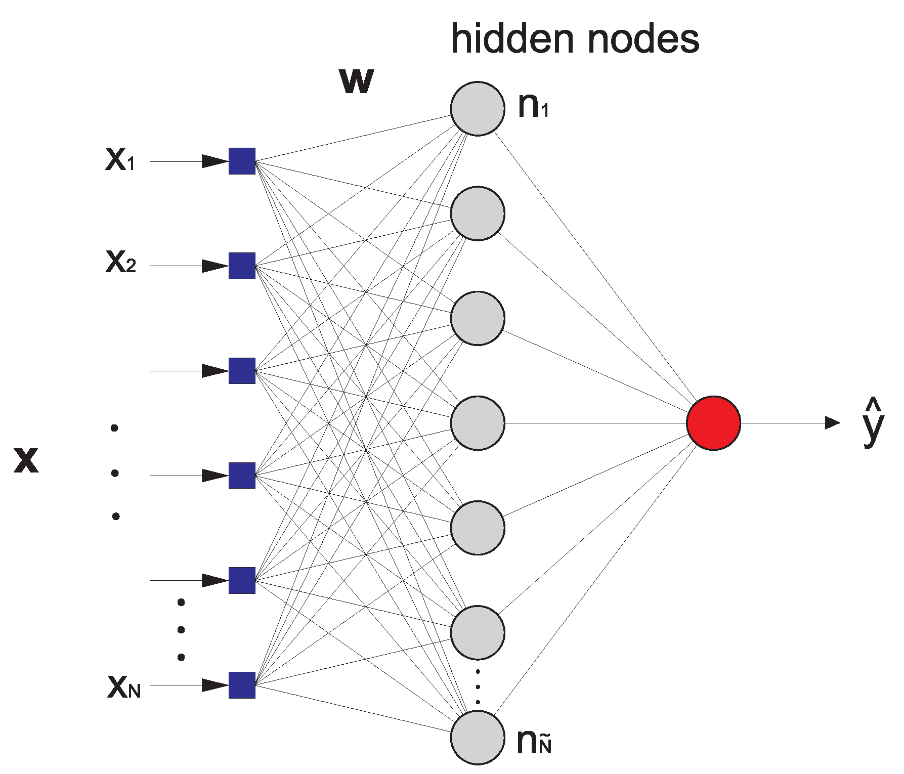
2.4.2. Extreme-Learning Machines

An extreme-learning machine [42] is a fast training method for neural networks, which can be applied to feed-forward perceptron structures, Figure 4. In the ELM, the network weights of the first layer are randomly set, and after this, a pseudo-inverse of the hidden-layer output matrix is obtained. This pseudo-inverse is then used to obtain the weights of the output layer which fit best with the objective values. The advantage of this method is not only that it is extremely fast, but also that it obtains competitive results versus other established approaches, such as classical training for multi-layer perceptrons, or even SVM algorithms, etc. The universal-approximation capability of the ELM have been proven in [43].
The ELM algorithm can be summarized by considering a training set { ( x i , y i ) | x i R N , y i { 1 , + 1 } , 1 i n } , an activation function g ( x ) , and a given number of hidden nodes N ˜ , and applying the following steps:
  • Randomly assign ELM weights values w i and the bias b i , where i = 1 , , N ˜ , according to a uniform probability distribution in the interval [ 1 , 1 ] .
  • Calculate the hidden-layer output matrix H , defined as follows:
    H = g ( w 1 x 1 + b 1 ) g ( w N ˜ x 1 + b N ˜ ) g ( w 1 x n + b 1 ) g ( w N ˜ x n + b N ˜ ) l × N ˜ .
  • Finally, calculate the output weight vector β as follows:
    β = H T ,
    where H is the Moore-Penrose inverse of the matrix H [42], and T is the training output vector, T = [ y 1 , , y n ] T .
Note that the number of hidden nodes N ˜ is a free parameter to be set before the training of the ELM algorithm, and must be estimated for obtaining good results by scanning a range of N ˜ . In this paper, we use the ELM implemented in Matlab by G. B. Huang, freely available at [47].

2.4.3. Synthetic Minority Over-Sampling Technique

Several studies have demonstrated that the treatment of the unbalanced data set samples improve the results obtained by the classifier’s training. Synthetic Minority Over-sampling Technique (SMOTE) [48] is a well-known technique for over-sampling the minority class in unbalanced classification problems. The objective is to increase the number of samples of the minority class by means of the formation of synthetic samples, working on the characteristics space. An over-sampling is applied to the minority class by means of the selection of every sample in this class and introducing synthetic samples as the k nearest neighbors (KNN) of the same class. Depending on the over-sampling applied, neighbors will be selected randomly from their KNN. In our case, a implementation with k = 5 is used. The generation process of the synthetic samples is as follows:
  • Let X = [ x 1 , , x N ] be a vector of characteristics and N the number of features.
  • Let X be a sample with N features for which its KNN are calculated.
  • Let Y be one of its KNN with the same size.
  • The synthetic sample, Z, would be:
    Z = X + ( X Y ) × D ,
    where D U ( 0 , 1 ) is a uniform random variable equally distributed in the interval ( 0 , 1 ) , which causes the selection of an aleatory point in the segment between two particular features.
This approach makes that the decision region of the minority class becomes most general. That is, SMOTE balances the series, equating the minority class with the majority class. This will avert the classification of the majority class more accurately than the minority class. The application of the SMOTE leads to important improvements in the results obtained for for the detection of low-visibility events, as can be seen in Section 3.2.

3. Experiments and Results

We present here the results of this study of low-visibility event persistence at Villanubla airport. We distinguish between long-term and show-term persistence, due to the different nature of their analyses: for long-term persistence, we show the results of the DFA approach, which provides its correlation exponent, α (see Section 2.2). The short-term persistence is evaluated by means of the MCM transition probabilities.
We also consider a short-term fog prediction problem, where the prediction capabilities of MCM and ML techniques are evaluated, in comparison to the Naïve persistence operator ( x ( t + 1 ) = x ( t ) ), which is a strong algorithm at short-term (hourly) scale. In this prediction problem, we have considered the following statistic metrics in order to evaluate the different prediction systems proposed: accuracy (ACC), true positive rate (TPR), true negative rate (TNR) and F1 score (F1S). For this problem, we represent a low-visibility event with a positive state (state 1) which corresponds with a RVR ≤ 2000 m. On the other hand, the absence of fog is represented with a negative state of the binary variable associated with RVR (state 0 or 1 for the ML algorithms). In the formulas describing the statistic metrics, we use the notation: TP ≡ True Positive; TN ≡ True Negative; FP ≡ False Positive; FN ≡ False Negative; P ≡ number of real positives; N ≡ number of real negatives.
ACC shows how close to the actual time series are the predicted time series. It is calculated as:
ACC = TP + TN P + N
TPR measures the proportion of actual positives that are correctly identified as positives:
TPR = TP TP + FN
TNR measures the proportion of actual negatives that are correctly identified as negatives:
TNR = TN TN + FP
Finally, the F1S is a measure of a test’s accuracy, and reaches its best value at 1:
F 1 S = 2 TP 2 TP + FP + FN
See references [49] and [50] for more details on these metrics.

3.1. Results: Long-Term Persistence Analysis

In order to evaluate the long-term persistence of low-visibility time series, we apply the DFA algorithm described in Section 2.2 to the complete time series of winter RVR, in the complete period considered (2008–2013) (Figure 5a), considering segments of length s = 5 h. The result of the DFA analysis carried out is shown in Figure 5b where the log-log graph of the fluctuation F ( s ) is depicted. It shows a marked long-term persistence, with two dominating scaling ranges, separated by a crossover at a characteristic time of 10 h. The DFA exponent below this crossover point is α = 1 . 37 > 0 . 5 , which reveals a very strong correlation of the RVR time series. Above this crossover point, the DFA exponent is α = 0 . 97 > 0 . 5 , which still shows a high correlation of the RVR time series, but smaller than below the 10 h characteristic time.

3.2. Results: Short-Term Persistence Analysis

Both the short-term persistence analysis and the subsequent fog prediction (classification problem) discussed in this paper, involve binary states of the fog event (fog/non-fog series). Thus, we have to binarize the RVR series. Let the series { x k | 1 k N } be the RVR time series considered. We then apply the following binarizing procedure:
s k = 1 if x k < 2000 ϵ { 0 / 1 } otherwise
where s k is the actual binary time series which depends on a given binarizing threshold ϵ (0 m in this case, so we consider as low-visibility event any visibilimeter measurement strictly under 2000 m). Recall that 2000 m is the observational limit of the visibilimeters at Valladolid airport (see Figure 5a above). The non-fog binary value could be 0 or 1 depending on the evaluated method (0 for MCM, but 1 for ML algorithms).
With this in mind, we report here the results obtained in the short-term persistence analysis of low-visibility events at Villanubla airport, and in the next section the results of the fog prediction problem. A K-fold cross-validation procedure has been carried out, to ensure that the results are independent from the partition in training and test data [51]. The folding has been set to K = 5 which corresponds to a 80 % to train and 20 % to test. Note that this data partition has been used both for this persistence analysis and also for the short-term prediction results reported in the next section.
In this case, the evaluation of the short-term persistence will be carried out by using the matrix of transition probabilities of the MCM, shown in Section 2.3. Note that the elements of the main diagonal can be used to estimate the persistence, as follows:
P = 1 2 ( p 00 + p 11 )
Note that in the case of higher-order MCM we estimate the short-term persistence as
P = 1 2 ( p α 0 0 + p α 1 1 )
where α 0 = ( 0 , , 0 ) stands for a tuple of N elements equal to 0, and α 1 = ( 1 , , 1 ) stands for a tuple of N elements equal to 1.
Table 2, Table 3, Table 4 and Table 5 show the transition probabilities and short-term persistence estimation (in the training set), for low-visibility events at Valladolid airport. It is possible to observe that low visibility events have a clear short-term persistence pattern, more pronounced when higher-order MCM are taken into account. As can be seen in Table 5 (4rd-order MCM), the persistence of the low visibility event, given that the four previous hours have had low visibility (i.e., event 1111 1 ), is over 87%. With this value, the total persistence P is near 92%. The short-term persistence pattern is clear even when the 1st order MCM is considered, in this case with a value of P close to 85%, though in this case the persistence of the low-visibility case (that is, the probability of transition from a foggy state to another foggy state, α 1 1 ) is lower than for higher-orders MCM, only 75 % (see Table 2).

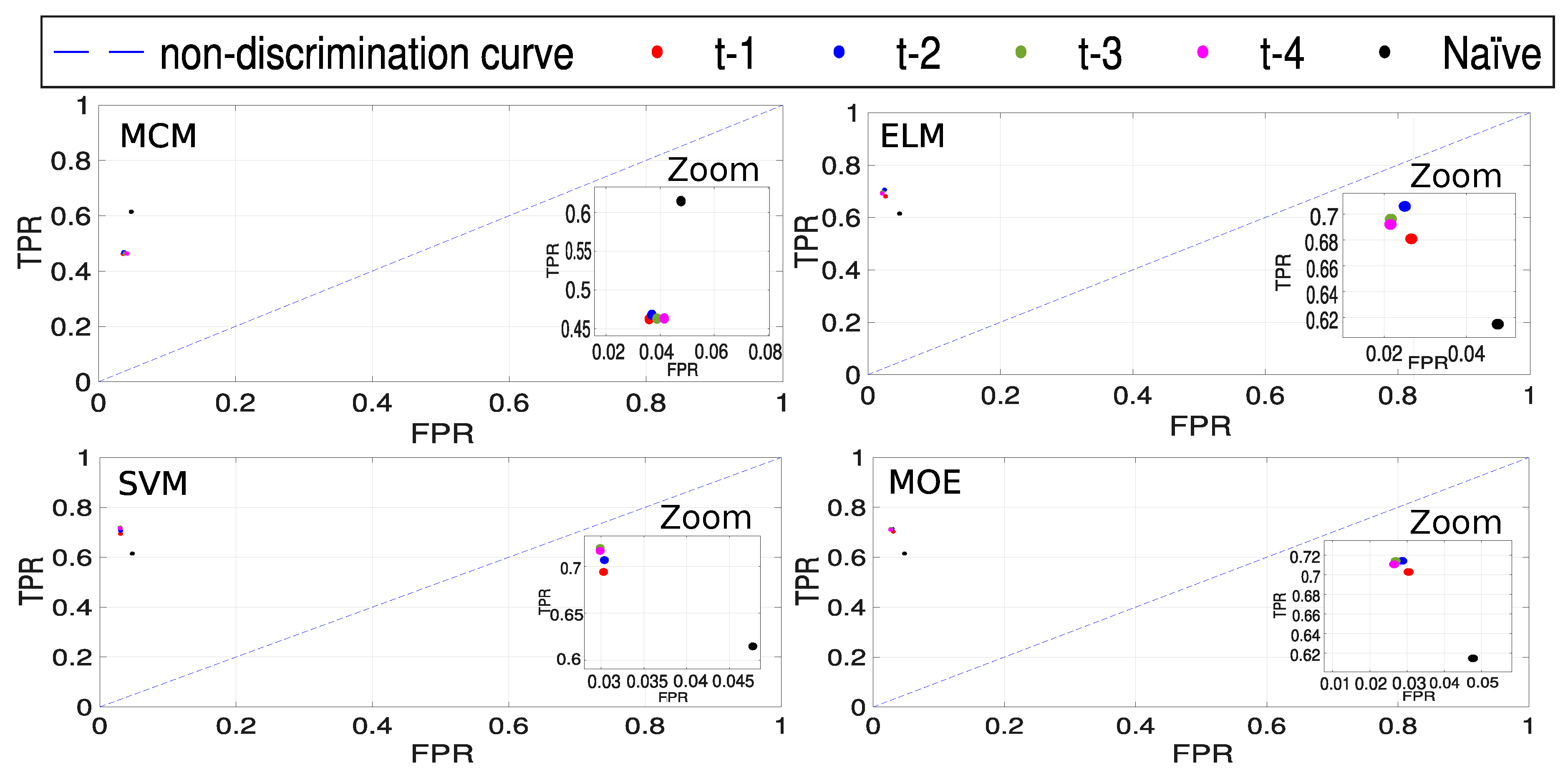
3.3. Results: Short-Term Prediction

Once we have shown the high persistence of the low-visibility phenomenon at Valladolid airport, we will test whether this property can be exploited to improve short-term low-visibility prediction in the zone, by solving a classification task.
First, note that a prediction exclusively based on previous values of low-visibility events (or in the binary states of the system) is possible by using the probability matrices of the MCM. In fact, we can use the Naïve persistence operator performance (obtained by means of a first-order MCM with transition matrix given by Equation (8)) as a baseline prediction algorithm. It obtains good results predicting low-visibility events with an hourly time window, as expected, with accuracy values over 0 . 92 . Note that, with this level of accuracy, the Naive persistence operator constitutes a very good prediction system, which is difficult to outperform even when adding exogenous variables.
The atmospheric state and dynamics will be considered in the prediction by means of the ML methods, which are trained with the input variables reported in Table 1. We will also consider both persistence and atmospheric state by means of the Mixture of Experts (MOE) approach. The idea of this analysis is to show that, in spite of persistence being extremely high in this problem, the use of hybrid models combining atmospheric state and persistence obtain the best results in the prediction of low-visibility events at Valladolid airport.
The result of the Naïve persistence operator (baseline algorithm) is compared to those by other techniques employed in this analysis for different time windows in the input data ( t 1 , t 2 , t 3 and t 4 ), see Table 6. Note that for the MCM and ELM approaches a Monte Carlo simulation of 30 runs (to ensure the statistical significance of the results) has been carried out, hence, the results are obtained from the mean of these 30 runs (the rest of the algorithms are deterministic, so it is not necessary to run them more than once). When the results of the different techniques have been obtained separately, we have prepared a MOE, where a majority voting from all methods involved gives the predicted RVR time series to compare with real data.
As it can be observed (see Table 6), the MCM is not able to beat the Naïve persistence operator, in spite of it having been trained with the real frequencies of low-visibility events occurrence. As previously mentioned, the ML approaches have the advantage of including external variables which take into account the atmospheric state. Both techniques (ELM and SVM) are able to overcome the Naïve operator, but the differences among them are small. It is possible to further improve the performance of ML approaches by using the Naïve operator as a basis and modifying it by means of other algorithms (ELM, SVM and MCM in this case) with a majority voting scheme (MOE system, as previously proposed in [18]). The MOE system is the best performing algorithm in this problem of short-term low-visibility event detection when considering a time window of t 1 . Note that if information from further time windows are considered ( t 2 , , t 4 ), the ELM with external information (atmospheric variables) is the best-over-all algorithm tested, with an accuracy of 0 . 94 .
If we represent the TPR against the false positive rate (FPR) in the ROC space [49] for each time window and for each technique employed, we can find that the results are always above the non-discrimination line (Figure 6), as expected. Note that the point in the upper left corner or coordinate (0,1) (perfect classification point) of the ROC space, represents 100% of sensitivity (absence of false negatives) and 100% specificity (absence of false positives) [49]. For a better visualization of the results obtained, a zoom has been obtained and included as figure insets for each model. It can be seen that the MCM is the only method which does not overcome the Naïve operator prediction performance (black point in the ROC space).
Table 7 represents the Euclidean distance between each point in Figure 6 and the perfect classification point, so that the smallest value gives the best prediction. Note that this is another way to justify what is the best time window to be considered for each method. For example, the MCM yields its best result when the t 2 time window is considered. The same situation occurs for ELM method. Finally, for the SVM and MOE the best result is obtained when a t 3 time window is considered for the input data. The highest distance is consistently obtained for t 1 in all cases. This means that the prediction is worse when a time window for the input data of just one hour is considered.

3.4. Discussion of the Results

The analysis of the long-term persistence of low-visibility events at Valladolid airport has been carried out with a DFA approach. The log-log plot of F ( s ) vs s has shown a clear two-ranges pattern, with two different DFA exponents ( α = 1 . 37 before 10 h and 0 . 97 after 10 h). In both cases, these α fulfil 0 . 5 < α < 1 , which means a strong long-persistence of the RVR time series, i.e., low-visibility events in winter at Villanubla airport. However, note that this result indicates that the persistence becomes so extreme below 10 h, that the time series exhibits non-stationary behavior ( α > 1 ). In previous works have associated these two ranges form of the DFA with the structure of a binary time series (fog/no-fog events) and its duration [52]. This suggests that the average returning time of low-visibility events in Valladolid airport at winter is, on average, 10 hours, and the long-term persistence of the events is very high ( α 1 for times over 10 h).
On the other hand, the study of short-term persistence has been focused on the analysis of the MCM transition probability matrices, for different time lags. We have shown that short-term persistence of low-visibility events is high, with values about 85% when considering one-hour time lag, to 92% for higher order MCM, up to 4 h time lag.
Regarding the short-term prediction problem tackled (classification task), we have carried out a comparison of different approaches, persistence-based and ML-based. First, we have shown the good performance achieved by the Naïve operator in this problem. Observe that the proposed Markov Chain models, based on probability matrices obtained from the real low-visibility event frequencies, are not able to outperform the Naïve operator. This indicates the existence of an extremely high persistence of the objective variable (RVR) at short-term time horizon prediction. ML algorithms with an over-sampling technique (SMOTE, see Section 2.4.3) are able to improve the Naïve operator results, adding some atmospheric state variables (external variables), strongly correlated with the appearance of fog events.
However, even considering ML algorithms with atmospheric variables, the obtained improvement versus the Naïve operator in terms of accuracy is small, 0 . 94 versus 0 . 92 respectively. Considering a time window of t 1 for the input data, the best results in terms of ACC are obtained by the MOE. By including variables at extra time windows ( t 2 , t 3 and t 4 ), the ELM slightly outperforms the MOE results, both better than the Naïve operator accuracy. Although the accuracy increment is small, ML algorithms achieve a TPR around 70 % , 10 % above the obtained by the Naïve operator, which constitutes a huge improvement of the low-visibility event predictions. A high TPR results in a better prediction of low-visibility events. The unbalanced classes between high-visibility states (over 2000 m) and low-visibility events, together with the low number of cases in which fog events change to high-visibility states, are responsible for the good performance of the Naïve operator in this problem.
These results show that the persistence of the low-visibility events at Valladolid is extreme at short-term time windows, where the Naïve operator is able to obtain a high performance and is very difficult to be defeated without external atmospheric extra information.

4. Conclusions

In this paper we have analyzed the persistence structure of low-visibility events at Villanubla airport using winter RVR time series at the airport as the objective variable. First, a long-term analysis of the RVR time series using a DFA approach has shown a long-term persistence of the series, with two dominating scaling ranges, separated by a crossover at a characteristic time of 10 h. The short-term persistence analysis has been studied by means of the Markov Chain probability transitions between states of fog/no-fog, obtaining a high degree of persistence in all cases analyzed. We have also discussed a prediction problem (classification task), where we have evaluated the role of persistence. Specifically we have carried out a comparison among different prediction methods, including persistence-based and ML algorithms with exogenous variables to take into account the atmospheric state. We have shown the prediction capabilities of a Naïve persistence operator in this problem, and how it can be hybridized with ML approaches to form a Mixture of Experts approach that is able to obtain highly accurate results in this problem.

Author Contributions

Conceptualization, S.S.-S., C.C.-M., A.J.C.; methodology, S.S.-S. and D.C.-P.; software, S.C.-B., L.C.-B., M.I.C. and D.C.-P.; validation, S.C.-B., L.C.-B, M.I.C., J.S.-J.; data curation, J.S.-J. and C.C.-M.; writing—original draft preparation, S.C.-B., S.S.-S., D.C.-P., A.J.C.; writing—revised draft, S.S.-S., D.C.-P., S.C.-B.; supervision, S.S.-S. All authors have read and agreed to the published version of the manuscript.

Funding

This research has been partially supported by the Ministerio de Economía, Industria y Competitividad of Spain (Grant Ref TIN2017-85887-C2-2-P and TIN2017-90567-REDT). This work has been also supported by the Universidad de Alcalá—ISDEFE Chair of Research in ICT and Digital Progress.

Conflicts of Interest

The authors declare no conflict of interest.

Abbreviations

The following abbreviations are used in this manuscript:
RVRRunway Visual Range
DFADetrended Fluctuation Analysis
MLMachine Learning
MCMMarkov Chain Model
MOEMixture of Experts
ELMExtreme Learning Machine
SVMSupport Vector Machine
SVSupport Vector
SMOTESynthetic Minority Over-sampling Technique
KNNk nearest neighbors
ACCAccuracy
TPRTrue Positive Rate
TNRTrue Negative Rate
F1SF1 score
TPTrue Positive
TNTrue Negative
FPFalse Positive
FPRFalse Positive Rate
FNFalse Negative
PNumber of real positives
NNumber of real negatives

References

  1. da Rocha, R.P.; Gonçalves, F.L.; Segalin, B. Fog events and local atmospheric features simulated by regional climate model for the metropolitan area of Sao Paulo, Brazil. Atmos. Res. 2015, 151, 176–188. [Google Scholar] [CrossRef]
  2. Huang, H.; Chen, C. Climatological aspects of dense fog at Urumqi Diwopu International Airport and its impacts on flight on-time performance. Nat. Hazards 2016, 81, 1091–1106. [Google Scholar] [CrossRef]
  3. Dey, S. On the theoretical aspects of improved fog detection and prediction in India. Atmos. Res. 2018, 202, 77–80. [Google Scholar] [CrossRef]
  4. Bergot, E.T.; Terradellas, J.; Cuxart, A.; Mira, O.; Liechti, M.; Mueller, N.; Nielsen, W. Intercomparison of single-column numerical models for the prediction of radiation fog. J. Appl. Meteor. Clim. 2007, 46, 504–521. [Google Scholar] [CrossRef]
  5. der Velde, I.V.; Steeneveld, G.; Wichers-Schreur, B.; Holtslag, A. Modeling and forecasting the onset and duration of severe radiation fog under frost conditions. Month. Weather Rev. 2010, 138, 4237–4253. [Google Scholar] [CrossRef]
  6. Zhou, B.; Du, J.; Gultepe, I.; Dimego, G. Forecast of low visibility and fog from NCEP: Current status and efforts. Pure App. Geoph. 2011, 169, 895–909. [Google Scholar] [CrossRef]
  7. Román-Cascón, C.; Yagüe, C.; Sastre, M.; Maqueda, G.; Salamanca, F.; Viana, S. Observations and WRF simulations of fog events at the Spanish northern plateau. Adv. Sci. Res. 2012, 8, 11–18. [Google Scholar] [CrossRef] [Green Version]
  8. Steeneveld, G.; Ronda, R.; Holtslag, A. The challenge of forecasting the onset and development of radiation fog using mesoscale atmospheric models. Bound. Layer Met. 2015, 154, 265–289. [Google Scholar] [CrossRef]
  9. Koziara, M.; Robert, J.; Thompson, W. Estimating marine fog probability using a model output statistics scheme. Month. Weather Rev. 1983, 111, 2333–2340. [Google Scholar] [CrossRef] [Green Version]
  10. Fabbian, D.; De-Dear, R.; Lellyett, S. Application of artificial neural network forecasts to predict fog at Canberra international airport. Weather Forecast. 2007, 22, 372–381. [Google Scholar] [CrossRef]
  11. Miao, Y.; Potts, R.; Huang, X.; Elliott, G.; Rivett, R. A fuzzy logic fog forecasting model for Perth Airport. Pure App. Geoph. 2012, 169, 1107–1119. [Google Scholar] [CrossRef]
  12. Colabone, R.O.; Ferrari, A.; da Silva-Vecchia, F.; Bruno-Tech, A. Application of artificial neural networks for fog forecast. J. Aerosp. Technol. Manag. 2015, 7, 240–246. [Google Scholar] [CrossRef]
  13. Boneh, T.; Weymouth, G.; Newham, P.; Potts, R.; Bally, J.; Nicholson, A.; Korb, K. Fog forecasting for Melbourne airport using a Bayesian decision network. Weather Forecast. 2015, 30, 1218–1233. [Google Scholar] [CrossRef]
  14. Dutta, D.; Chaudhuri, S. Nowcasting visibility during wintertime fog over the airport of a metropolis of India: Decision tree algorithm and artificial neural network approach. Nat. Hazards 2015, 75, 1349–1368. [Google Scholar] [CrossRef]
  15. Cornejo-Bueno, L.; Casanova-Mateo, C.; Sanz-Justo, J.; Cerro-Prada, E.; Salcedo-Sanz, S. Efficient prediction of low-visibility events at airports using Machine-Learning regression. Bound. Layer Met. 2017, 165, 349–370. [Google Scholar] [CrossRef]
  16. Guijo-Rubio, D.; Gutiérrez, P.A.; Casanova-Mateo, C.; Sanz-Justo, J.; Salcedo-Sanz, S.; Hervás-Martínez, C. Prediction of low-visibility events due to fog using ordinal classification. Atmos. Res. 2018, 214, 64–73. [Google Scholar] [CrossRef]
  17. Fernández-González, S.; Bolgiani, P.; Fernández-Villares, J.; González, P.; Garcá-Gil, A.; Suarez, J.C.; Merino, A. Forecasting of poor visibility episodes in the vicinity of Tenerife Norte Airport. Atmos. Res. 2019, 223, 49–59. [Google Scholar] [CrossRef]
  18. Perez-Ortiz, M.; Gutierrez, P.A.; Tino, P.; Casanova-Mateo, C.; Salcedo-Sanz, S. A mixture of experts model for predicting persistent weather patterns. In Proceedings of the International Joint Conference on Neural Networks, Rio de Janeiro, Brazil, 8–13 July 2018. [Google Scholar]
  19. Bunde, A.; Havlin, S.; Koscielny-Bunde, E.; Schellnhuber, H.J. Longterm persistence in the atmosphere: Global laws and tests of climate models. Physica A 2001, 302, 255–267. [Google Scholar] [CrossRef]
  20. Bunde, A.; Havlin, S. Power-law persistence in the atmosphere and in the oceans. Physica A 2002, 314, 15–24. [Google Scholar] [CrossRef] [Green Version]
  21. Pelletier, J.D.; Turcotte, D.L. Long-range persistence in climatological and hydrological time series: Analysis, modeling and application to drought hazard assessment. J. Hydrol. 1997, 203, 198–208. [Google Scholar] [CrossRef]
  22. Yang, L.; Fu, Z. Process-dependent persistence in precipitation records. Physica A 2019, 527, 121459. [Google Scholar] [CrossRef]
  23. Koçak, K. Practical ways of evaluating wind speed persistence. Energy 2008, 33, 65–70. [Google Scholar] [CrossRef]
  24. Gadian, A.; Dewsbury, J.; Featherstone, F.; Levermore, J.; Morris, K.; Sanders, C. Directional persistence of low wind speed observations. J. Wind Eng. Ind. Aerodyn. 2004, 92, 1061–1074. [Google Scholar] [CrossRef]
  25. Jiang, L. Mean wind speed persistence over China. Physica A 2018, 502, 211–217. [Google Scholar] [CrossRef]
  26. Zhang, W.F.; Zhao, Q. Asymmetric long-term persistence analysis in sea surface temperature anomaly. Physica A 2015, 428, 314–318. [Google Scholar] [CrossRef]
  27. Voyant, C.; Notton, G. Solar irradiation nowcasting by stochastic persistence: A new parsimonious, simple and efficient forecasting tool. Renew. Sustain. Energy Rev. 2018, 92, 343–352. [Google Scholar] [CrossRef] [Green Version]
  28. Harrouni, S.; Guessoum, A. Using fractal dimension to quantify long-range persistence in global solar radiation. Chaos Sol. Fract. 2009, 41, 1520–1530. [Google Scholar] [CrossRef]
  29. Morales-Rodriguez, C.; Ortega-Villazan, M. Approximation to the study of fogs in middle Duero valley. Geogr. Res. 1994, 12, 23–44. [Google Scholar]
  30. AEMET. Aeronautical Climatology of Valladolid/Villanubla; Technical Report; Agencia Estatal de Meteorología: Madrid, Spain, 2015. [Google Scholar]
  31. CPeng, K.; Buldyrev, S.V.; Havlin, S.; Simons, M.; Stanley, H.E.; Goldberger, A.L. Mosaic organization of DNA nucleotides. Phys. Rev. E 1994, 49, 1685–1689. [Google Scholar]
  32. Peng, C.K.; Havlin, S.; Stanley, H.E.; Goldberger, A.L. Quantification of scaling exponents and crossover phenomena in nonstationary hear beat time series. Chaos 1995, 5, 82–87. [Google Scholar] [CrossRef]
  33. Li, J.M.; Wei, H.J.; Wei, L.D.; Zhou, D.P.; Qiu, Y. Extraction of frictional vibration features with multifractal Detrended Fluctuation Analysis and Friction State recognition. Symmetry 2020, 12, 272. [Google Scholar] [CrossRef] [Green Version]
  34. Hu, K.; Ivanov, P.C.; Chen, Z.; Carpena, P.; Stanley, H.E. Effect of Trends on Detrended Fluctuation Analysis. Phys. Rev. E 2001, 011114. [Google Scholar] [CrossRef] [PubMed] [Green Version]
  35. Graves, T.; Gramacy, R.; Watkins, N.; Franzke, C. A Brief History of Long Memory: Hurst, Mandelbrot and the Road to ARFIMA, 1951–1980. Entropy 2017, 19, 437. [Google Scholar] [CrossRef] [Green Version]
  36. Mann, M.E. On long range dependence in global surface temperature series. Clim. Chang. 2011, 107, 267–276. [Google Scholar] [CrossRef]
  37. Wilks, D.S. Statistical Methods in the Atmospheric Sciences; Academic Press: Cambridge, MA, USA, 2011; Volume 100. [Google Scholar]
  38. Cazacioc, L.; Cipu, E.C. Evaluation of the transition probabilities for daily precipitation time series using a Markov chain model. In Proceedings of the 3rd International Colloquium-Mathematics in Engineering and Numerical Physics, Bucharest, Romania, 7–9 October 2004; Volume 12, pp. 82–92. [Google Scholar]
  39. Katz, R.W. Precipitation as a Chain-Dependent Process. J. Appl. Met. 1977, 16, 671–676. [Google Scholar] [CrossRef] [Green Version]
  40. Cristianini, N.; Shawe-Taylor, J. An Introduction to Support Vector Machines and Other Kernel-Based Learning Methods; Cambridge University Press: New York, NY, USA, 2000. [Google Scholar]
  41. Salcedo-Sanz, S.; Rojo, J.L.; Martínez-Ramón, M.; Camps-Valls, G. Support vector machines in engineering: An overview. WIREs Data-Min. Know. Disc. 2014, 4, 234–267. [Google Scholar] [CrossRef]
  42. Huang, G.B.; Zhu, Q.Y. Extreme learning machine: Theory and applications. Neurocomputing 2006, 70, 489–501. [Google Scholar] [CrossRef]
  43. Huang, G.B.; Zhou, H.; Ding, X.; Zhang, R. Extreme Learning Machine for Regression and Multiclass Classification. IEEE Trans. Syst. Man Cybern. Part B 2012, 42, 513–529. [Google Scholar] [CrossRef] [PubMed] [Green Version]
  44. Pérez-Ortiz, M.; Jiménez-Fernández, S.; Gutiérrez, P.A.; Alexandre, E.; Hervás, C.; Salcedo-Sanz, S. A review of classification problems and algorithms in renewable energy applications. Energies 2016, 9, 607. [Google Scholar] [CrossRef]
  45. Schölkopf, B.; Smola, A. Learning with Kernels—Support Vector Machines, Regularization, Optimization and Beyond; MIT Press: Cambridge, MA, USA, 2002. [Google Scholar]
  46. Bhartendu, MATLAB Central File Exchange. Available online: https://www.mathworks.com/matlabcentral/fileexchange/63158-support-vector-machine (accessed on 18 December 2019).
  47. Huang, G.B. ELM Matlab Code. Available online: http://www.ntu.edu.sg/home/egbhuang/elm_codes.html (accessed on 22 June 2020).
  48. Chawla, N.V.; Bowyer, K.W.; Hall, L.O.; Kegelmeyer, W.P. SMOTE: Synthetic minority over-sampling technique. J. Artif. Intel. Res. 2002, 16, 321–357. [Google Scholar] [CrossRef]
  49. Fawcett, T. An introduction to ROC analysis. Pattern Rec. Lett. 2006, 27, 861–874. [Google Scholar] [CrossRef]
  50. Sasaki, Y. The truth of the F-measure. Teach Tutor Mater 2007, 1, 1–5. [Google Scholar]
  51. Kohavi, R. A study of cross-validation and bootstrap for accuracy estimation and model selection. Int. Jt. Conf. Artif. Intell. 1995, 14, 1137–1145. [Google Scholar]
  52. Matsoukas, C.; Islam, S.; Rodriguez-Iturbe, I. Detrended fluctuation analysis of rainfall and streamflow time series. J. Geophys. Res. 2000, 205, 165–172. [Google Scholar] [CrossRef]
Figure 1. Location of Villanubla airport, Valladolid, Spain; (a) Location in the Iberian Peninsula; (b) Orography of Valladolid area.
Symmetry 12 01045 g001
Figure 2. Diagrams representing a two-state (a) First-order; (b) N-order Markov process.
Symmetry 12 01045 g002
Figure 3. Support Vector Machine (SVM) Illustration: Linear decision hyperplane in a non-linearly transformed feature space H . The slack variables ξ i are included to define the soft-margin.
Symmetry 12 01045 g003
Figure 4. Multi-layer perceptron structure considered in the Extreme Learning Machine (ELM) algorithm.
Symmetry 12 01045 g004
Figure 5. Runway Visual Range (RVR) time series and Detrended Fluctuation Analysis (DFA) carried out; (a) RVR time series in winter at Villanubla airport; (b) DFA obtained from the analysis. The DFA exponent is 1 . 37 in times under 10 h, and 0 . 97 over this characteristic time, which indicates the strong correlation of the RVR signal.
Symmetry 12 01045 g005
Figure 6. ROC space and plots of the methods considered for different time windows in the input data ( t 1 , , t 4 ), and the Naïve persistence operator; (a) MCM; (b) ELM; (c) SVM; (d) Mixture of Experts (MOE). An enlarged view is represented in the insets. Note that the exact location of the points is given in the zoomed insets.
Symmetry 12 01045 g006
Table 1. Description of the input variables considered in the Machine Learning (ML) algorithms.
VariableHeight above the Ground (m)UnitsInstrument
Temperature97, 96.6, 35.5, 20.5, 10, 10.5, 2.3, 2 CRiso P2448A and P2642A
Relative Humidity97, 10, 2%Vaissala HMP45A
Wind speed98.6, 74.6, 34.6, 9.6, 2.2m/sRiso P2548A
Wind direction98.6, 74.6, 34.6, 9.6degrees trueRiso P2021A
Atmospheric pressure2hPaVaisala PA21
RVR (target)2mVaisala FD12
Table 2. Transition probabilities for the 1st order Markov Chain Models (MCM). Boldface figures stand for p 00 and p 11 , respectively.
P = 1 2 ( P 00 + P 11 )

85.47 %
01
095.574.43
124.6375.37
Table 3. Transition probabilities for the 2nd order MCM. Boldface figures stand for p 00 0 and p 11 1 , respectively.
P = 1 2 ( p 00 0 + p 11 1 )

89.82 %
01
0095.904.10
0150.2249.78
1088.6011.40
1116.2683.74
Table 4. Transition probabilities for the 3rd order MCM. Boldface figures stand for p 000 0 and p 111 1 , respectively.
P = 1 2 ( p 000 0 + p 111 1 )

91.36 %
01
00096.014.00
00151.8548.15
01091.178.83
01131.5268.48
10093.256.75
10137.3062.70
11086.0114.00
11113.2986.71
Table 5. Transition probabilities for the 4th order MCM. Boldface figures stand for p 0000 0 and p 1111 1 , respectively.
P = 1 2 ( p 0000 0 + p 1111 1 )

91.76%
01
000096.133.87
000150.5449.46
001091.198.81
001133.4566.55
010094.415.59
010145.4954.51
011090.049.96
011117.6982.31
100093.226.78
100169.7730.23
101090.439.56
101120.1379.87
110092.027.98
110131.9168.09
111084.1915.81
111112.6287.38
Table 6. Statistical measurements for all the methods tested in this problem of low-visibility events prediction.
Time WindowModelACCTPRTNRF1S
t− 1MCM0.90530.46270.96410.5510
ELM0.92990.68080.97340.7409
SVM0.93000.69410.96980.7427
MOE0.93060.70280.96960.7479
t− 2MCM0.90890.46820.96310.5533
ELM0.93540.70590.97500.7625
SVM0.93110.70670.96960.7501
MOE0.93370.71410.97130.7594
t− 3MCM0.90840.46330.96120.5452
ELM0.93700.69600.97840.7633
SVM0.93400.71960.97010.7619
MOE0.93560.71400.97310.7644
t− 4MCM0.90660.46350.95850.5383
ELM0.93640.69190.97850.7613
SVM0.93330.71650.97010.7593
MOE0.93520.71050.97350.7632
t− 1Naïve0.92510.61480.95230.6421
Table 7. Euclidean distance between each data point and the perfect classification point, for each time window and method considered.
MCMELMSVMMOE
t− 10.53850.32030.30740.29875
t− 20.53310.29520.29490.28733
t− 30.53810.30480.28200.28726
t− 40.53810.30880.28510.29071

