Landslide Susceptibility Mapping Using the Slope Unit for Southeastern Helong City, Jilin Province, China: A Comparison of ANN and SVM

1
College of Construction Engineering, Jilin University, Changchun 130026, China
2
Jilin Team of Geological Survey Center of China Building Materials Industrial, Changchun 130026, China
*
Author to whom correspondence should be addressed.
Symmetry 2020, 12(6), 1047; https://0-doi-org.brum.beds.ac.uk/10.3390/sym12061047
Submission received: 1 June 2020
/
Revised: 19 June 2020
/
Accepted: 21 June 2020
/
Published: 23 June 2020
Abstract
:The purpose of this study is to produce a landslide susceptibility map of Southeastern Helong City, Jilin Province, Northeastern China. According to the geological hazard survey (1:50,000) project of Helong city, a total of 83 landslides were mapped in the study area. The slope unit, which is classified based on the curvature watershed method, is selected as the mapping unit. Based on field investigations and previous studies, three groups of influencing Factors—Lithological factors, topographic factors, and geological environment factors (including ten influencing factors)—are selected as the influencing factors. Artificial neural networks (ANN’s) and support vector machines (SVM’s) are introduced to build the landslide susceptibility model. Five-fold cross-validation, the receiver operating characteristic curve, and statistical parameters are used to optimize model. The results show that the SVM model is the optimal model. The landslide susceptibility maps produced using the SVM model are classified into five grades—very high, high, moderate, low, and very low—and the areas of the five grades were 127.43, 151.60, 198.77, 491.19, and 506.91 km2, respectively. The very high and high susceptibility areas included 79.52% of the total landslides, demonstrating that the landslide susceptibility map produced in this paper is reasonable. Consequently, this study can serve as a guide for landslide prevention and for future land planning in the southeast of Helong city.
1. Introduction
Landslides are one of the most common geological disasters in the mountainous areas of China [1,2,3]. In recent years, the Chinese economy has developed steadily and rapidly, and has become the second largest economy in the world. With such rapid development of the economy, many previously inaccessible areas have carried out corresponding infrastructure construction and various engineering activities in succession. Therefore, it is necessary to evaluate the risk of natural disasters such as landslides in these areas. Landslide susceptibility mapping is the basis of landslide hazard and risk assessment [4]. The purpose of landslide susceptibility mapping is to answer the question “what is the geological background of landslides and where are the areas which are most prone to them?” [2]. Based on the review of relevant papers, it was found that landslide susceptibility mapping mainly includes the following [5,6]: (a) landslide inventory data acquisition; (b) mapping unit selection; (c) influencing factor selection; (d) establishment of the evaluation model; and (e) production of the landslide susceptibility map.
Landslide inventory data is the basis of landslide susceptibility mapping. The early acquisition of landslide inventory data mainly depends on field geological disaster surveys. With the development of remote sensing technology, landslide interpretation based on remote sensing technology has become one of the most popular tools to quickly acquire landslide inventory data [7,8]. Remote sensing techniques commonly used in landslide interpretation mainly include (a) visible optical remote sensing and (b) InSAR (Interferometric Synthetic Aperture Radar) remote sensing. The key to remote sensing interpretation of landslides based on visible optics is to interpret the landslide based on the special topographic and geomorphic features of the landslide in the remote sensing image. However, this method is greatly affected by the spatial resolution of remote sensing data and is unable to identify the surface deformation characteristics (i.e., the potential and slow deformation of the landslide); thus, it has certain limitations. However, landslide interpretation based on InSAR technology can effectively identify the surface deformation and identify the potential landslides that are under deformation [9], which makes up for the limitations of visible optical remote sensing interpretation. The combination of these two methods has become a common method for landslide interpretation. As for mapping units, they are the basic units in landslide susceptibility mapping [10]. At present, the commonly used mapping units are the grid unit, watershed unit, slope unit, region unit, and uniform condition unit [4]. Among these, the grid unit is the most widely used but, due to its lack of connection with the topography and other geological information, the slope unit [11,12] has become more and more respected by relevant scholars. The selection of influencing factors is one of the key issues in the study of landslide susceptibility mapping [13]. The choice of influencing factors used in the evaluation will affect the final mapping results. The selection of influencing factors mostly relies on field investigation, cause analysis, expert experience, and related research of landslides; the factors with the highest correlation with the occurrence of landslides in the study area are typically selected as the influencing factors to evaluate the susceptibility to landslides [2]. At present, many scholars also use methods of automatic forward selection of parameters that weight and evaluate the effectiveness of each influencing factor and make use only of the “best” ones [14,15]. The evaluation models applied to landslide susceptibility mapping are mainly divided into qualitative and quantitative evaluation [6,16]. Qualitative evaluation is mainly based on the knowledge and experience of relevant experts, where the susceptibility to geological hazards such as landslides is determined by means of grading and weighting [17,18]. Quantitative evaluation methods include statistics, machine learning, deep mining, and other methods [6]. With the rapid improvement of calculation ability, an increasing number of quantitative evaluation methods have been applied to landslide susceptibility mapping. In addition, evaluation methods of the performance of landslide susceptibility models have also been developed rapidly [16,19]. Finally, the landslide susceptibility map can be produced according to the established model.
According to the basic steps of landslide susceptibility mapping, this paper carries out a relative evaluation of the southeast of Helong City, Jilin Province, northeastern China. Firstly, according to the geological hazard survey (1:50,000) project, 83 landslides were mapped in the study. Then, the slope unit classified by the curvature watershed method was applied as the mapping unit, which can identify the horizontal surface and the inclined surface. Moreover, the area of the slope unit is more concentrated, the shapes mostly range between isosceles triangles and squares, and there are few elongated units. Next, ten influencing factors were selected. Artificial neural networks (ANN) and support vector machines (SVM) were introduced to build the landslide susceptibility model. Five-fold cross-validation, the receiver operating characteristic curve (ROC), and statistical parameters were used to optimize the model. Finally, the landslide susceptibility map was divided into five classes. This study can serve as a guide for landslide prevention and for future land planning in the southeast of Helong city.
2. Study Area
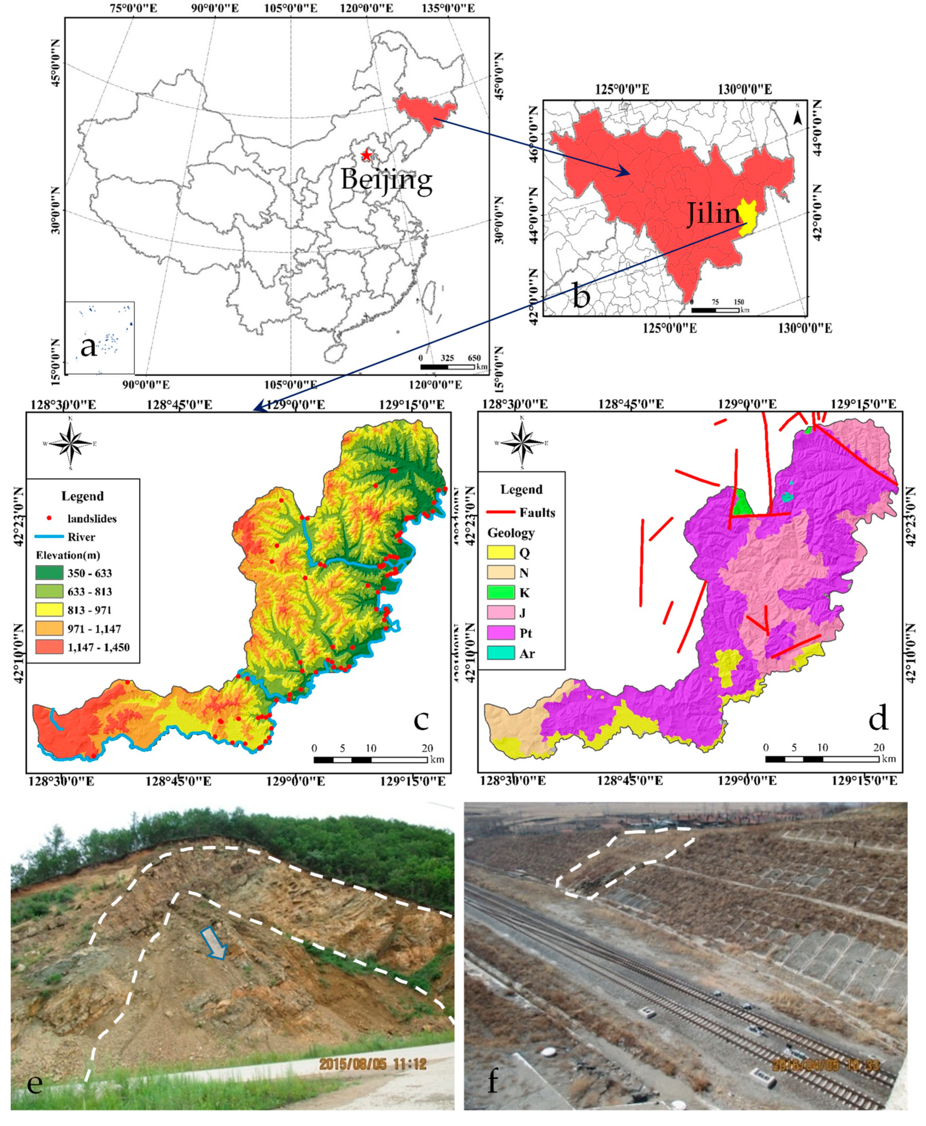
The study area is in the Chongshan and Nanping counties of the southeast Helong city, Jinlin province, China, along the Tumen river. The study area is marked by valleys and rugged topography, and covers an area of 1476 km2 (Figure 1a–c). More than 90% of the total area of the study area consists of mountainous areas. In the study area, the maximum elevation is 1450 m, and the minimum elevation is 350 m. The southern part of the study area is the Chinese and Korean quasi-platform, and the northern part is the Jihei fold system in the Tianshan-Xingan geosyncline fold area, which are bounded by the deep and large fault of Gudong River. The study area belongs to the temperate monsoon sub-humid climate zone. Based on rainfall data collected from 1960 to 2012, the maximum daily rainfall of the study area is 164.8 mm. The perennial average temperature is 5.6 °C. The vegetation coverage in the study area is relatively high. The seismic intensity of the study area has a degree of VI on the modified Mercalli index. At present, no earthquake-induced landslides have been detected in the study area. According to the field investigation, the landslides in the study area are mainly distributed along the Tumen River. According to a geological map (downloaded using the 91 Weitu software, with a scale of 1:500,000) (Figure 1d), it can be seen that the mainly exposed strata in the study area are Quaternary (Q), Neogene (N), Cretaceous (K), Jurassic (J), Middle Proterozoic (Pt), and New Archean (Ar). The lithological information of the study area is listed in Table 1. There are several reverse faults in the study area, which affect the regional stability. The Tumen river and its tributaries flow through the study area, which has a significant impact on landslide risk.
3. Methodology
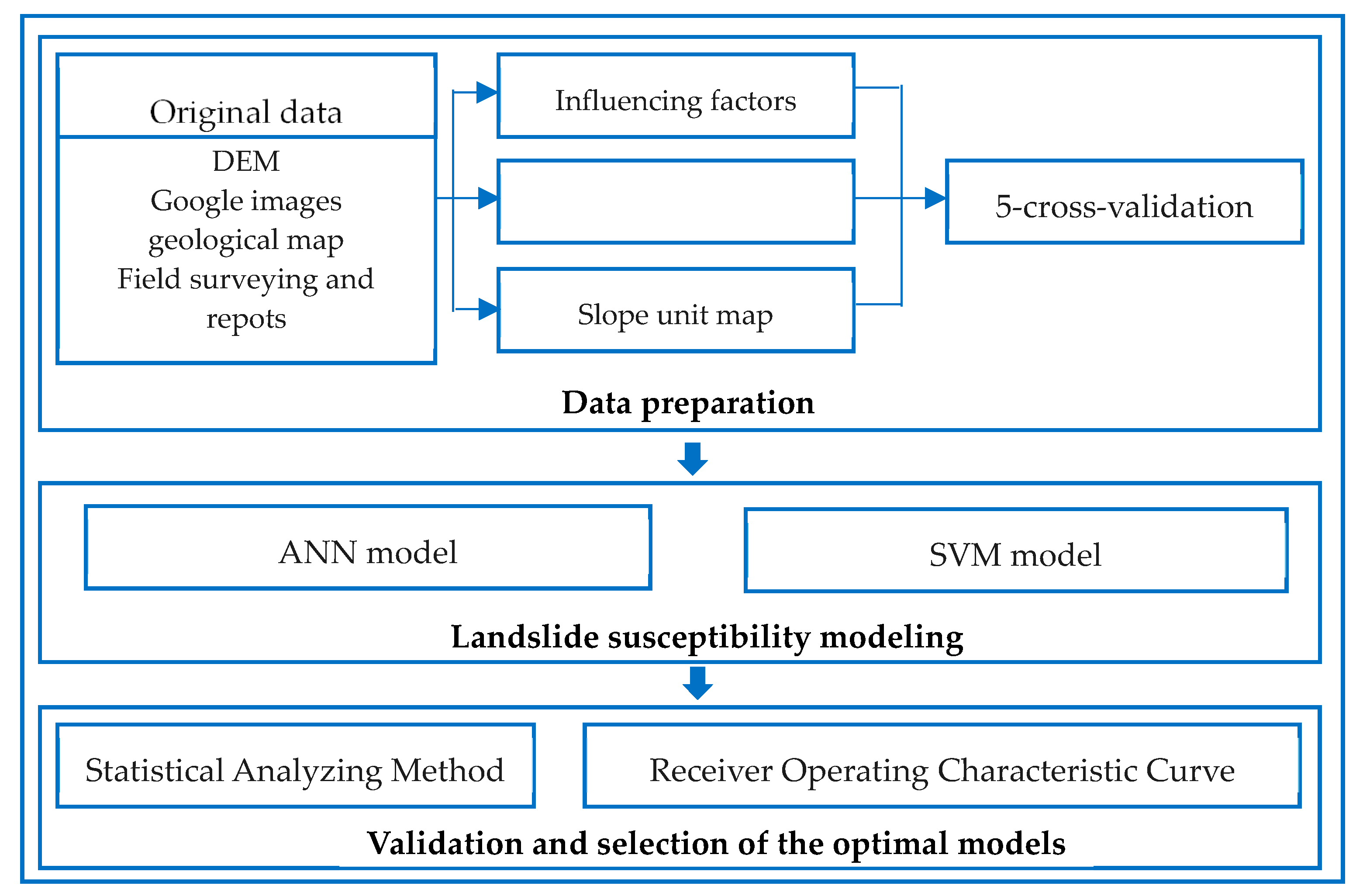
Figure 2 shows the three main steps of this paper, namely (a) data preparation, (b) landslide susceptibility modelling, and (c) validation and selection of the optimal models.
3.1. The Mapping Unit
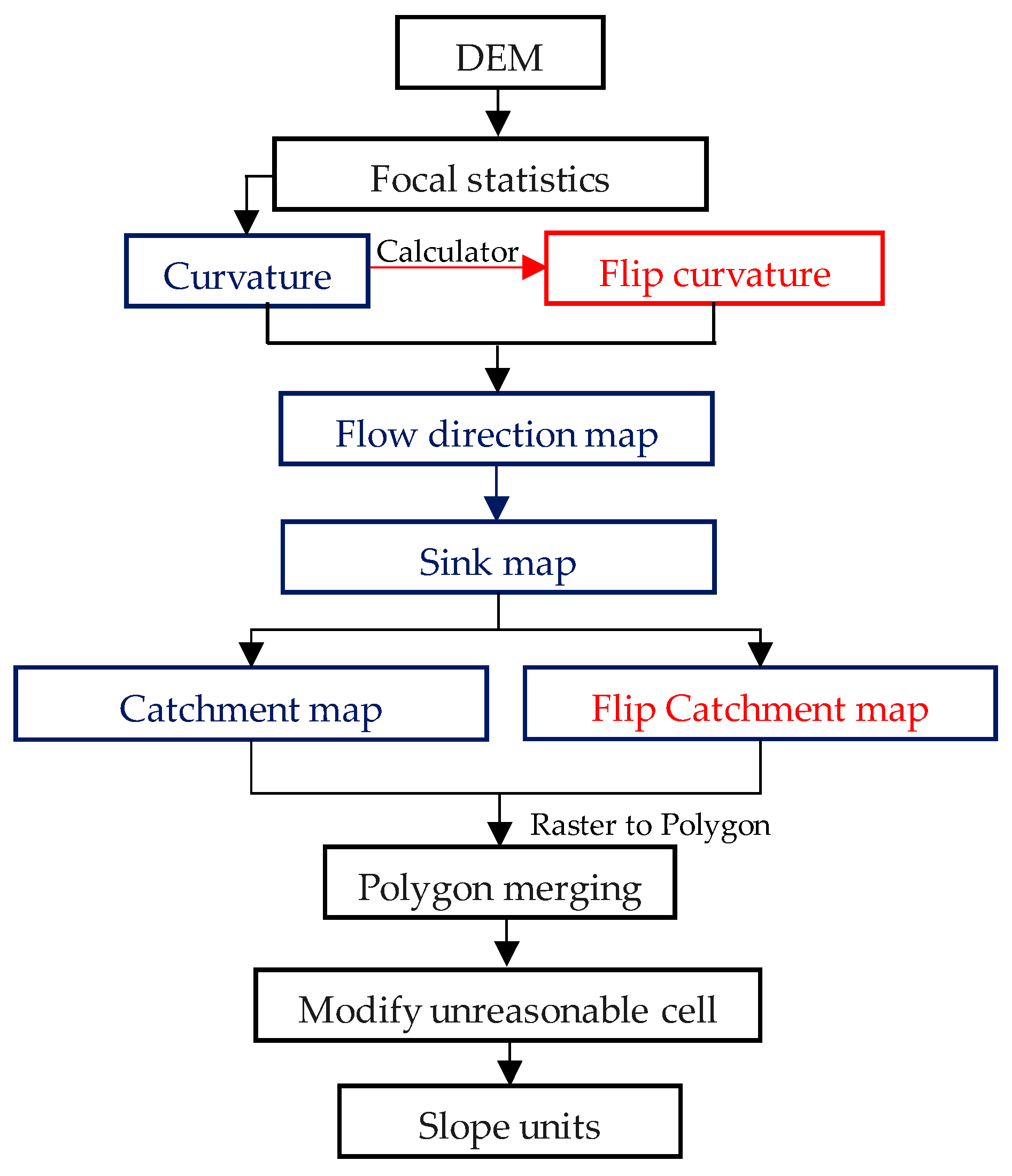
Reasonable mapping units should be determined before landslide susceptibility mapping is carried out [20]. Whether the mapping unit is reasonable or not directly affects the accuracy of the final evaluation result. Slope units are often used to study landslide susceptibility mapping due to their close relationship with the topography. The dividing principle of slope units is to divide the research area into many small areas with different sizes by cutting along the ridge and valley lines [21]. At present, hydrologic analysis is the most used method for dividing slope units. However, this method cannot identify the boundary between the horizontal and the inclined surface and generates a large number of parallel river networks, which increases the difficulty of manual modification [21]. By comparing the slope unit division results of the curvature watershed method and the hydrologic analysis method, it was found that the slope unit divided based on the curvature watershed method has a uniform size, a regular shape, and small terrain variation inside, which is obviously better than the result based on the hydrological method. Therefore, we chose the curvature watershed method to divide the slope units in this study. Slope units are divided by valley and ridge lines, where there are abrupt changes in slope angle and slope aspect. Therefore, slope units can be divided according to the change of slope angle and slope aspect. Profile curvature and plan curvature are the derivatives of slope angle and slope aspect, respectively. Their maximum and minimum values can reflect abrupt changes of slope angle and slope aspect. Therefore, the curvature can be used to divide the slope units. The specific process of dividing slope units based on curvature is shown in Figure 3. It is mainly used to identify the boundary of concave terrain and convex terrain by the curvature and reverse curvature, respectively, to divide the slope units. The classification steps of the slope units can be divided into two parts: positive relief extraction and negative relief extraction. The original curvature was used to extract the positive relief, and the flip curvature was used to extract the negative relief, which can be obtained by multiplying the curvature by −1. Before calculating the curvature, to remove the influence of the roughness of the original Digital Elevation Model (DEM) on the curvature calculation results, focal statistics were made on the DEM with three pixels as the radius. After the flow direction and sink calculations, the positive and negative relief boundary can be obtained. The results of dividing slope units can be obtained by merging the positive and negative relief boundaries and manually modifying the unreasonable units.
3.2. Landslide Inventory
Landslide inventory data is the basis of landslide susceptibility mapping. In order to grasp the spatial distribution characteristic information and develop a mechanism of landslide hazards in the study area, the Jilin team of the Geological Survey Center of China Industrial Building Materials carried out the geological hazard survey (1:50,000) project of Helong city. The characteristic geomorphological features of the landslides, such as the chair-like landform of the landslide, a color difference between the landslide and the surrounding environment, and a change of vegetation before and after the landslide, can be clearly identified in a remote sensing image. Thus, the project team preliminarily identified 112 landslides in the study area using the visible optical remote sensing technology and Google images. Then, during the field geological survey, the remote sensing interpretation results were reviewed, and 42 interpretation results were excluded (such as exposed steep cliffs of bedrock and a waste rock dump in a quarry) and the uninterpreted landslides were supplemented. Finally, a total of a total of 83 landslides were mapped in the study area (Figure 1c), including soil and rock slope deformation, soil slide, and collapse. Figure 1e,f are examples of the landslides. Table A1 shows the basic information for the landslides. According to Table A1, the landslides in the study area are mostly rock landslides, which are mainly developed in crystalline rocks. These landslides are mainly controlled by the rock mass structural plane, and a small number of landslides are controlled by the contact surface between the overburden layer and the rock mass. The scale of landslide is mainly small and medium size. The failure mode of the landslides is mainly pull-type and toppling-type.
3.3. Influencing Factors
The occurrence of a landslide is a complicated process. Therefore, the factors influencing the occurrence of a landslide are also varied. Pourghasemi and Rossi [13] reviewed a total of 220 related papers and found that the factors with the highest application frequency in landslide susceptibility mapping were slope angle, lithology, slope aspect, land use, distance to river, elevation, distance to faults, curvature, distance to road, and soil type, among others. The selection of influencing factors for the landslide susceptibility mapping in the study area should be based on the understanding of the characteristics of the landslide and the geological environment. Therefore, the relationship between the landslide and the geological environment in the study area was analyzed as follows.
3.3.1. Relationship between Geological Environment and Landslides
Relationship between Topographic Features and Landslides
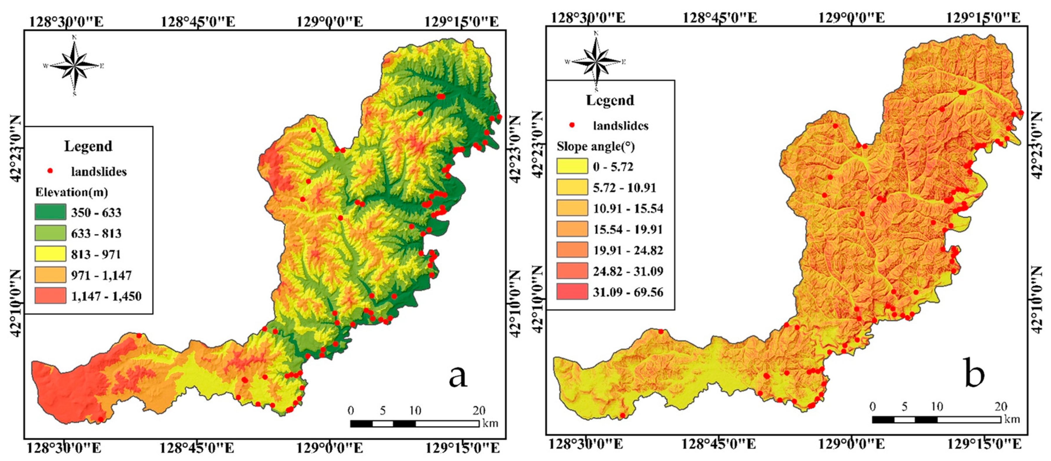
The topography is the basic condition of a landslide and determines the formation and development of landslide to a great extent. For example, convex and bedding slopes are prone to landslides. Based on field investigation and analysis, it was found that most landslides in the study area occurred in hills and low mountains with an elevation range of 200–1000 m and a slope angle more than 30° (Figure 4). Furthermore, the number of landslides increased with the increase of the slope angle. The number of landslides in a convex slope was much larger than that in concave slope. The micro-landform of the landslide site was a steep slope or steep coast (Table A1).
Relationship between Lithological Features and Landslides
The lithology of landslides in the study area was mainly crystalline rocks, such as granite, diorite, and other magmatic rocks (Table A1). The number of landslides in the crystalline rock in the study area was the largest and was obviously higher than that in other geotechnical rock type distribution areas. This is because the crystalline rock is usually strongly influenced by joints, cracks, and faults. The presence of these structural planes greatly reduces the shear strength of the rock mass, resulting in the sliding of the upper rock mass or overlying loose rock.
Relationship between Geologic Features and Landslides
The number of landslides in fault geological tectonic units was the largest in the study area. This is mainly because the in-situ stress of the fracture is stronger than that of other parts, and its influence range is larger and wider. The rock in these parts has deformations such as bending, squeezing, and tearing, which reduces the structural mechanical properties of the rock mass.
Relationship between Rainfall Features and Landslides
According to statistics, the landslides that occurred in the study area were mostly caused by heavy rainfall, and the two are positively correlated. Continuous heavy rainfall, particularly during the flood season, results in a high incidence of landslides.
Relationship between Other Features and Landslides
Landslides occurred more frequently in areas with low vegetation coverage in the study area. Landslides occurred extensively along the Tumen river, which is the main river in the study area. Earthquakes are an important trigger of landslides. They damage the integrity of rock and soil mass and make slopes prone to landslide. However, there is no historical record of landslides triggered by earthquakes in the study area. Thus, seismic activity has had little effect on the occurrence of landslides in the study area.
3.3.2. Selection of Influencing Factors
Based on the above analysis, and the statistical results of Pourghasemi and Rossi [13], three groups of influencing factors were selected for this study: geologic factors, topographic factors, and environment factors. The geologic factors only consist of geology, while there were five topographic factors: elevation, slope angle, slope aspect, topographic relief, and curvature. Finally, there were four environment factors: land use, rainfall, distance to river, and distance to faults. In this study, all the influencing factor maps were extracted using the slope unit. Furthermore, the dominant category of lithology, land use, was estimated as the influencing factor value of each slope unit, with the average value used for the other factors.
3.3.3. Extraction of Influencing Factors
Geologic Factor
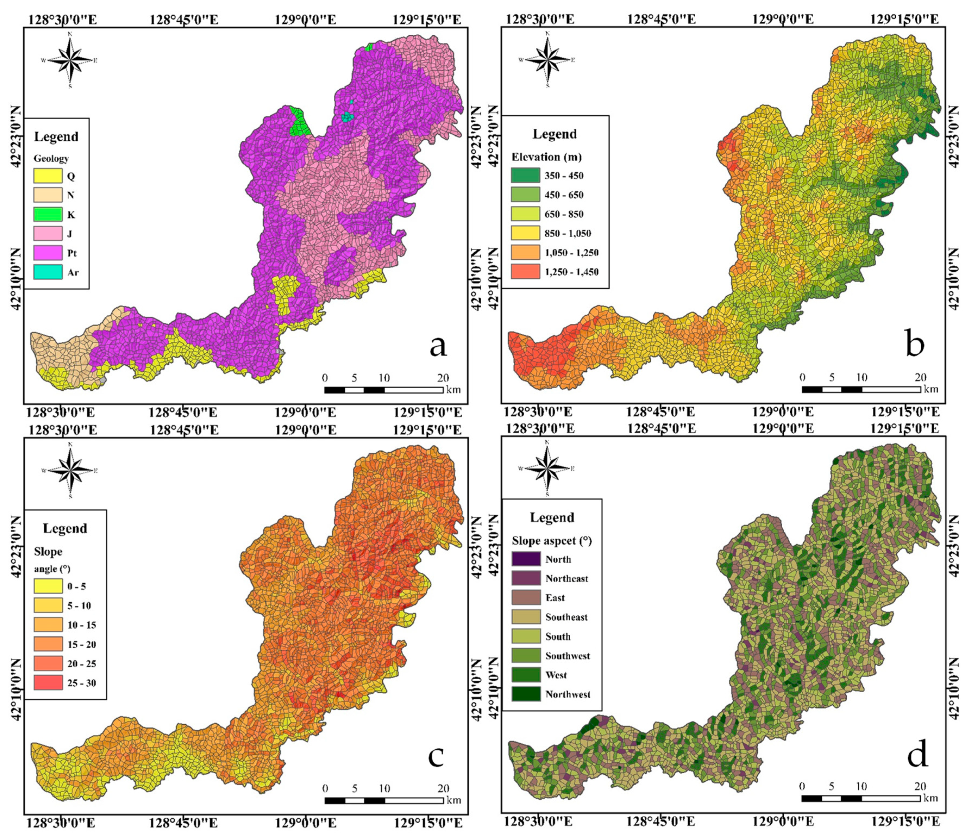
The study area is covered with six types of geologic formations, composed of different lithologies pertaining to different geologic ages. The combination of these two characteristics is one of the most important factors influencing the occurrence of landslides [22]. The shear strength, weathering resistance, and crushing degree of different lithologies are greatly different [23]. In addition, the same lithology with different structural planes will have different effects on the stability of the slope. A rock mass with joint and fissure development is more prone to landslides than a complete rock mass. A highly weathered rock mass is also less stable than a fresh rock mass. In this study, the geology map was obtained based on a geological map with a scale of 1:500,000 (downloaded using 91 Weitu software); the geology map of the study area is shown in Figure 5a.
Topographic Factors
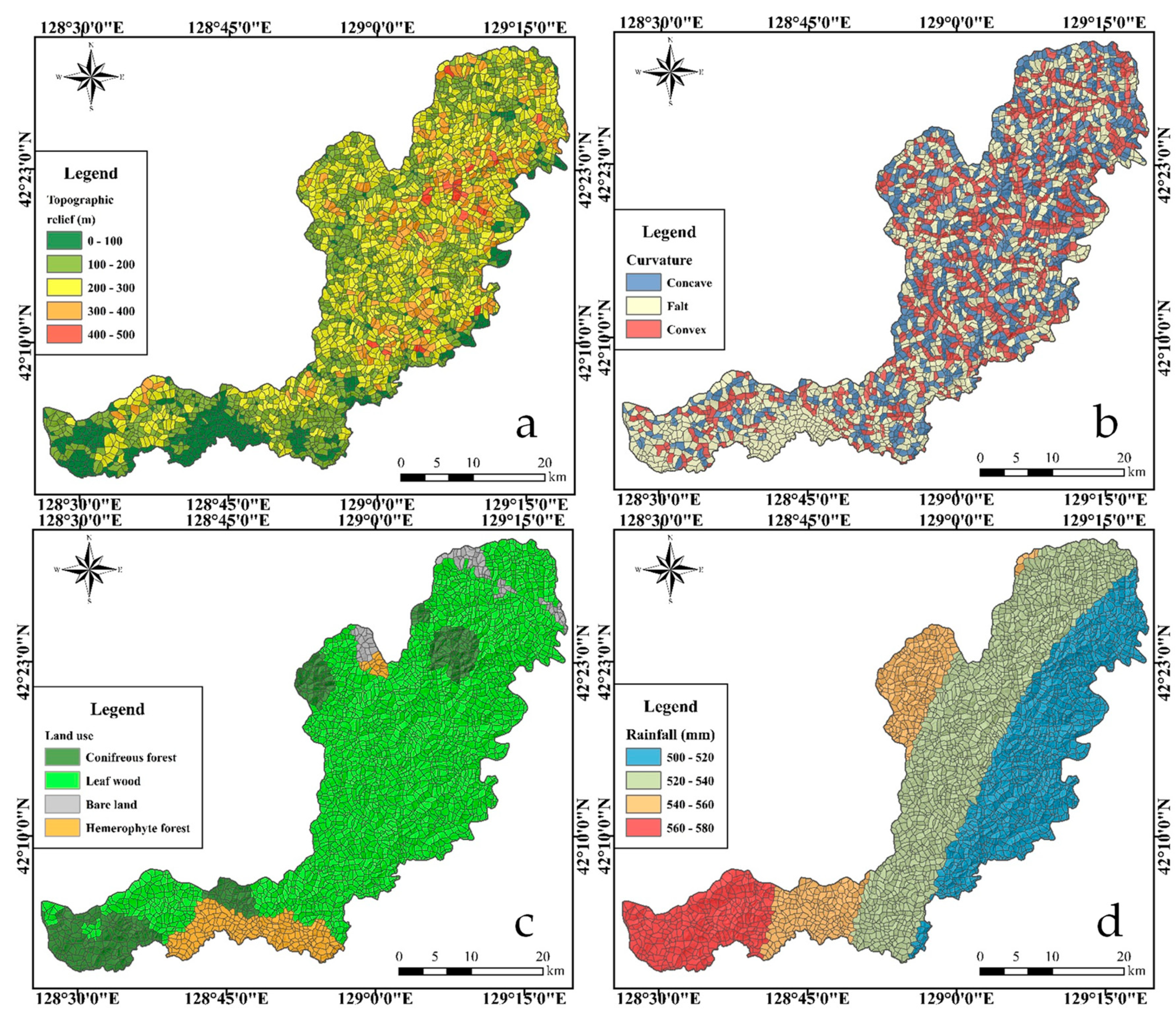
Elevation usually affects the depth of the water table aquifer [1,24]. In addition, the higher the elevation, the less human activity takes place, which is also more conducive to the stability of the slope. Regarding the slope angle, a change of slope angle changes the original stress state of the slope [25]. Within a certain range of slope, the self-gravity stress and shear stress in the slope generally increase with an increase of the slope angle, and the probability of slope instability increases accordingly. The intensity of light exposure, the type and extent of vegetation cover, and the supply of surface water vary greatly with differing slope aspect [2,26]. For example, the illumination time on a sunny slope is much longer than that on a shady slope; therefore, the temperature difference between day and night on a sunny slope is also larger than that on a shady slope and the dry–wet cycle is also faster. In this case, the weathering strength of the rock mass on a sunny slope is larger than that on a shady slope, which reduces the strength and stability of rock and soil mass on the sunny slope, in turn increasing the probability of landslide [4]. The topographic Relief—The difference between the highest and lowest Points—Can reflect the degree of relief in a specific area [4]. Curvature can reflect the shape of a slope body. According to the shape characteristics, a slope can be divided into three forms: convex slope, straight slope, and concave slope [27]. A DEM (Digital Elevation Model) with a resolution of 10 × 10 m was used to extract the five influencing factor maps through the slope unit using ArcGis software. The five influencing factor maps are shown in Figure 5b–d and Figure 6a,b.
Environment Factors
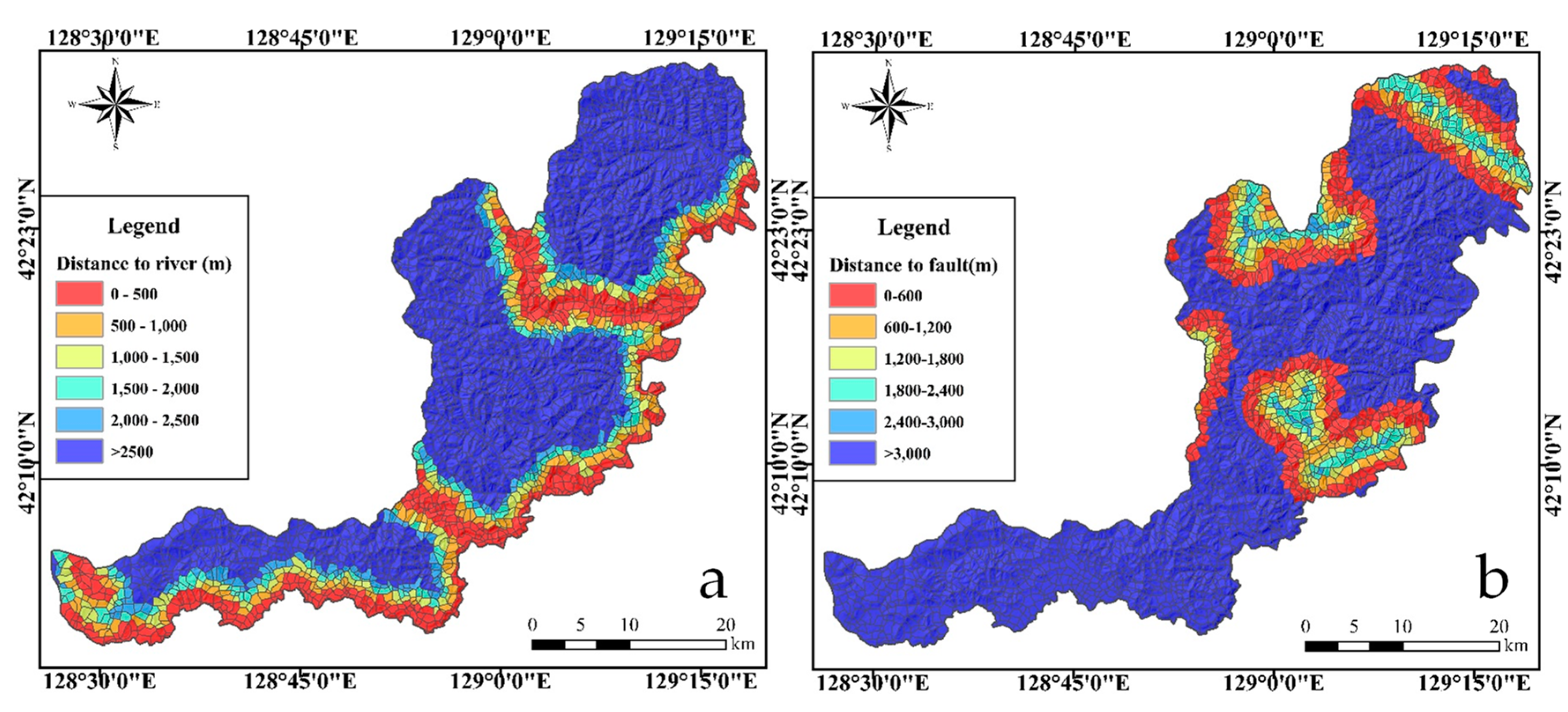
Vegetation has a positive effect on the stability of a slope, which can enhance the resistance of the slope surface to water erosion and influence rainfall infiltration. Rainfall has a significant impact on slope risk. Rainwater infiltration will increase the gravity of rock and soil mass, reducing their shear strength parameters, which will have an adverse effect on slope stability. The distance to river factor has an important influence on the occurrence of landslides [28]. The downcut of a river increases the slope angle along the river. To adapt to the rapid downcut, disasters such as landslides often occur along the river, thus reducing the slope angle. The existence of faults leads to the development of joints and fissures in the surrounding rock mass, which leads to fragmentation of the rock mass and a reduction of weathering resistance [29]. Therefore, many geological hazards such as landslides often develop around deep and large fissures. These four influencing factors are extracted through the slope unit using ArcGis software. The five influencing factor maps are shown in Figure 6c,d and Figure 7a,b.
3.4. Landslide Susceptibility Modeling
At present, an increasing number of models are being applied to the study of landslide susceptibility mapping [30,31,32,33]. Each of these models has its advantages and disadvantages; combined with the complexity of the factors affecting slope stability and the different geological environments in different regions, it is impossible to apply one model to the study of landslide susceptibility in all areas. Therefore, in the relevant evaluation of the study area, the evaluation model adopted should be optimized to determine the most suitable landslide susceptibility evaluation model. Recently, some machine learning approaches have been developed with the aim of evaluating the landslide susceptibility [21]. Due to its strong learning ability, fast calculation speed, and strong fault tolerance, the artificial neural network (ANN) model has become one of the most used machine learning methods in landslide susceptibility mapping. By comparison, the support vector machine (SVM) model requires fewer modeling data and is suitable for binary classification problems. Thus, the SVM model may be more suitable for landslide susceptibility prediction with fewer data, such as in the case of this study. Therefore, we selected the artificial neural network (ANN) and support vector machine (SVM) models to optimize the evaluation model of landslide susceptibility in the study area.
3.4.1. Artificial Neural Network (ANN)
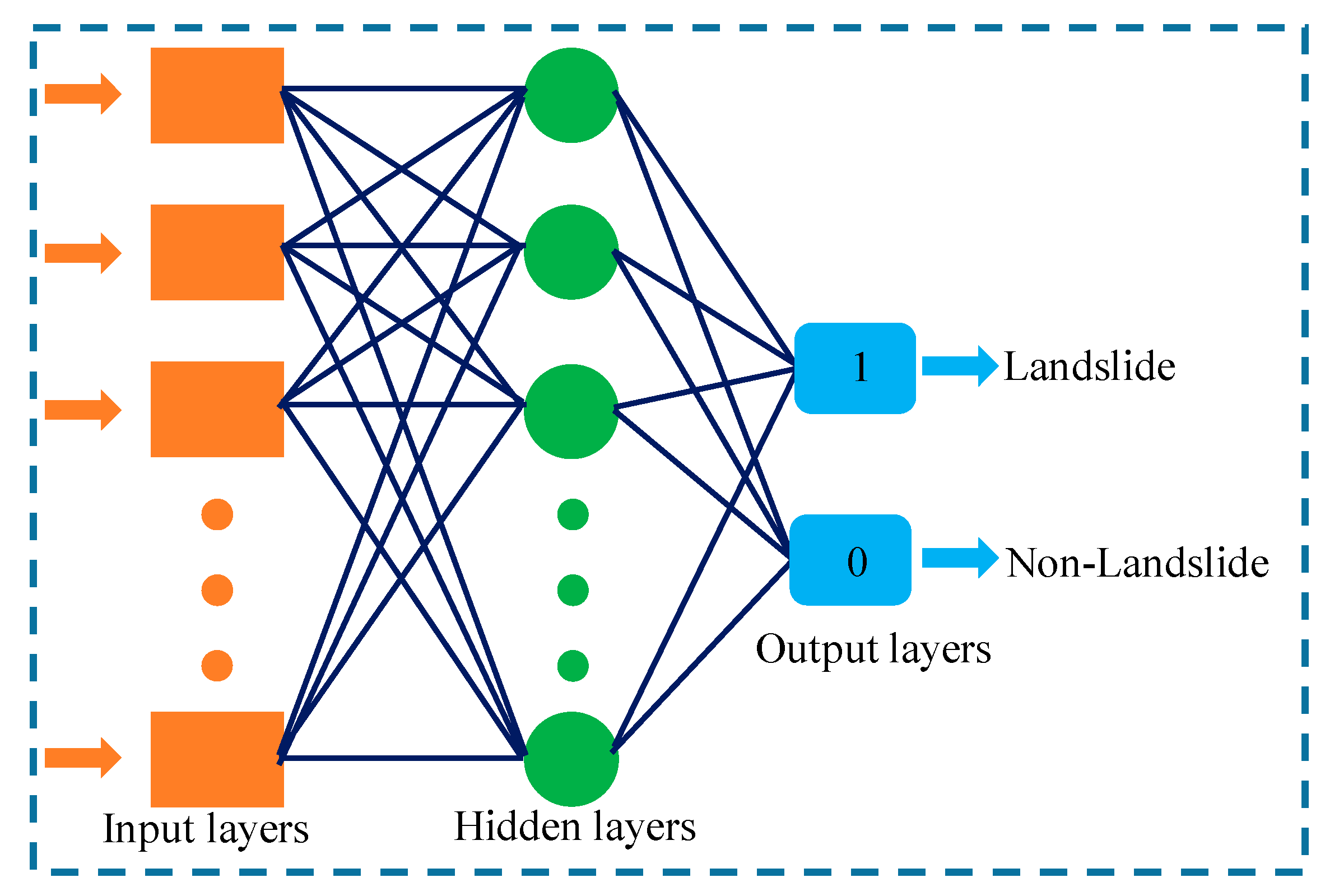
As a machine learning method, the artificial neural network model has been widely used in the study of landslide susceptibility mapping [26,34,35]. The ANN model has the following advantages [36]: (a) better non-linear mapping capability; (b) highly self-learning and adaptive; (c) strong generalization ability; and (d) strong fault tolerance. Thus, the ANN model can simulate the complex non-linear interactions between influencing factors and landslides through the interaction between neurons. Moreover, in an ANN model it is not necessary to describe the interactions between factors by complex mathematical formulae [37]. The fitting effect is relatively good, which is especially suitable for the simulation of complex geological phenomena influenced by many factors and presents advantages for the simulation of phenomena such as landslides, in which various factors interact and have complex relationships. A complete artificial neural network model is usually composed of an input layer, an output layer, and one or more hidden layers. Figure 8 shows a schematic diagram of a simple artificial neural network model. Each layer contains several of the model’s basic units: neurons. The data processing and storage of an artificial neural network are represented as the mutual relationships and connections between neurons. Through training using samples, the ANN changes the weights of its internal connections to minimize the error between the output value and the target value, to achieve the purpose of accurate modeling. Each node in the input layer corresponds to a predictive variable, while the node in the output layer corresponds to the target variable. A hidden layer is a regular layer connecting the input layer and output layer, and the number of the hidden layers and the number of nodes in each layer determine the complexity of the network. The process of forecasting with an ANN can be divided into a learning process and a prediction process [38]. The learning process, in which a large number of learning samples and the iterative function of the network are used to train the network by optimizing the process via minimizing the network error, includes the forward transmission of input information and the reverse transmission of error [34]. The prediction process is the process of substituting the unknown sample into the model after training. According to the rules of the learning sample, the process finally obtains the output result of the sample through the forward transmission of the input information [39].
3.4.2. Support Vector Machine (SVM)
The support vector machine (SVM) model is also a machine learning model. Its theoretical basis is statistical learning theory [40,41,42,43]. The SVM model has the following advantages [40,44]: (a) low data volume requirement; (b) strong generalization ability; (c) strong optimization ability; (d) adaptability to high-dimensional samples; and (e) strong learning ability and fast convergence. It can realize the linear segmentation of data by transforming each evaluation index from low dimensional space to high dimensional space. Thus, it can analyze and evaluate non-linear problems in low dimensional space. Due to its low requirement in terms of data volume, it has also been widely used in the study of landslide susceptibility mapping. The process of modeling for landslide susceptibility evaluation by SVM is summarized as follows [40,44]:
Consider some linearly separable data points xi (i = 1, 2,…,n) that fall into two different classes yi = ±1. The goal of SVM is to find a hyperplane in n-dimensional data space which can separate the two classes of data based on the maximum interval. The hyperplane can be expressed mathematically as follows:
which should satisfy the following constraint conditions:
where ||w|| is the norm of the normal vector of the hyperplane, b is a scalar, and represents the scalar product. Based on the Lagrange multiplier, the cost function can be expressed as follows:
where λi is the Lagrange multiplier.
In the case of linear indivisibility, the constraint condition can introduce a slack variable ξi, which can be expressed as follows:
Then, Equation (1) can be converted into the following form:
In Equation (5), v in [0,1] is introduced to consider the case of misclassification. In addition, the kernel function K (xi, yi) is introduced to explain the non-linear decision boundary problem in SVM.
3.5. Data for Landslide Susceptibility Modeling
When using an artificial neural network or support vector machine to establish a landslide susceptibility model, the same amount of data is needed for landslide units and non-landslide units. In this study, we determined the number of slope units with landslides according to the division results of slope units in the study area and the landslide inventory map. An equal number of units were randomly selected at a minimum distance of 800 m from these units, in order to avoid the effects of landslides [37]. The five-fold cross-validation method [39,40] was used to validate the models and to overcome the shortage of landslide data and the problem of model overfitting. All the ten influencing factors were involved in landslide susceptibility model building.
3.6. Validation Method
3.6.1. Receiver Operating Characteristic Curve (ROC)
The receiver operating characteristic curve (ROC) [18,45] is a quantitative analysis method to evaluate the prediction accuracy of the landslide susceptibility model. This method evaluates the prediction accuracy of the model using the area under the curve (AUC). The AUC value lies between 0 and 1, and the greater its value, the higher the prediction accuracy of the model.
3.6.2. Statistical Analysis Method
Statistical indices are also widely used for evaluating the prediction ability of landslide susceptibility mapping models [21]. The most used statistical indices are the following:
where Ac is the accuracy; Sen is the sensitivity; Sp is the specificity; PPV is the positive predictive value; NPV is the negative positive value; TP is the true positive; TN is the true negative; FP is the false positive; and FN is the false negative.
4. Results
4.1. Division Result of the Slope Units
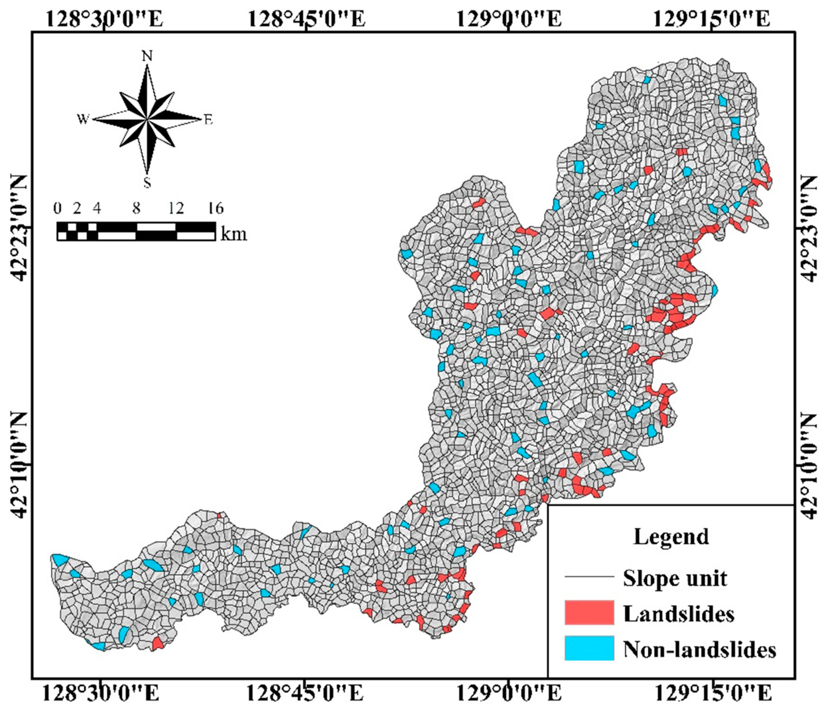
In this paper, a DEM with a resolution of 10 × 10 m was adopted to the divided slope units of the study area. In the process of division, we found that the size of slope units divided by the curvature watershed method was related to the DEM resolution. Therefore, the DEM resolution was converted to 10 × 10 m, 30 × 30 m, 50 × 50 m, 80 × 80 m, 100 × 100 m, and 120 × 120 m for slope classification. By comparing the slope unit classification results with Google images of the study area, it was found that the slope unit classification result was the most consistent with the actual terrain with the DEM with a resolution of 80 × 80 m. A total of 2956 slope units were obtained (Figure 9). The maximum area of a slope unit was 18.45 × 10⁵ m2 and the minimum area was 0.11 × 10⁵ m2.
4.2. Model Fitting Results
According to the landslide inventory map, there are 83 slope units containing the entire known landslide body. Therefore, the 83 slope units that experienced landslides were used as the modeling data. To meet the modeling requirements, the same number of non-landslide units (83) were randomly selected at least 800 m away from the landslide units (Figure 9). To establish the ANN model, the numbers of input, hidden, and output layers should be determined first. In this study, each of the input, hidden, and output layers consisted of a single layer. Secondly, the number of neurons in each layer was determined, with the number of neurons in the input layer the same as the number of influencing factors. There were ten influencing factors used for modeling in this study, thus, the number of neurons in the input layer was ten. The output layer was used to determine whether a landslide occurs, so the number of neurons was two. The number of hidden layer neurons can be determined by the following empirical formula [46]:
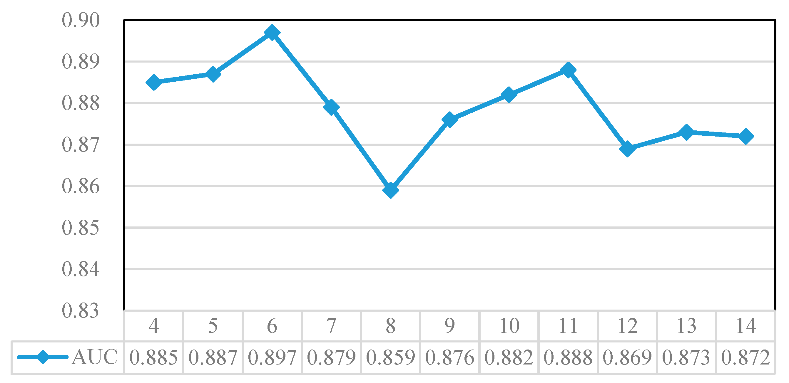
where N is the recommended value for the number of neurons in the hidden layer, A is the number of neurons in the input layer, B is the number of neurons in the output layer, and k is an empirical coefficient with value between 0 and 10. According to the empirical formula, the ideal number of hidden layer neurons in the artificial neural network in this study ranged from 4 to 14. By using all the data to establish the ANN model, the number of hidden layer neurons was optimized. It can be seen from Figure 10 that, when the number of hidden layer neurons is 6, the ANN model has the highest prediction accuracy. Thus, the number of neurons in the hidden layer was finally selected as 6.
For the ANN model, the learning rate, momentum, and training time were set as 0.3, 0.3, and 500, respectively [34,37]. The choice of kernel function affects the prediction accuracy of SVM. In this study, the radial basis function (RBF) was selected as the kernel function, which was influenced by the regularization parameter (C) and the kernel parameter (g). C and g were set as 0.8 and 0.5 [34,47,48], respectively. All the parameters were obtained based on the previous research experience and experiments in the calculation process. The model fitting results are shown in Table 2.
4.3. Landslide Susceptibility Mapping Results
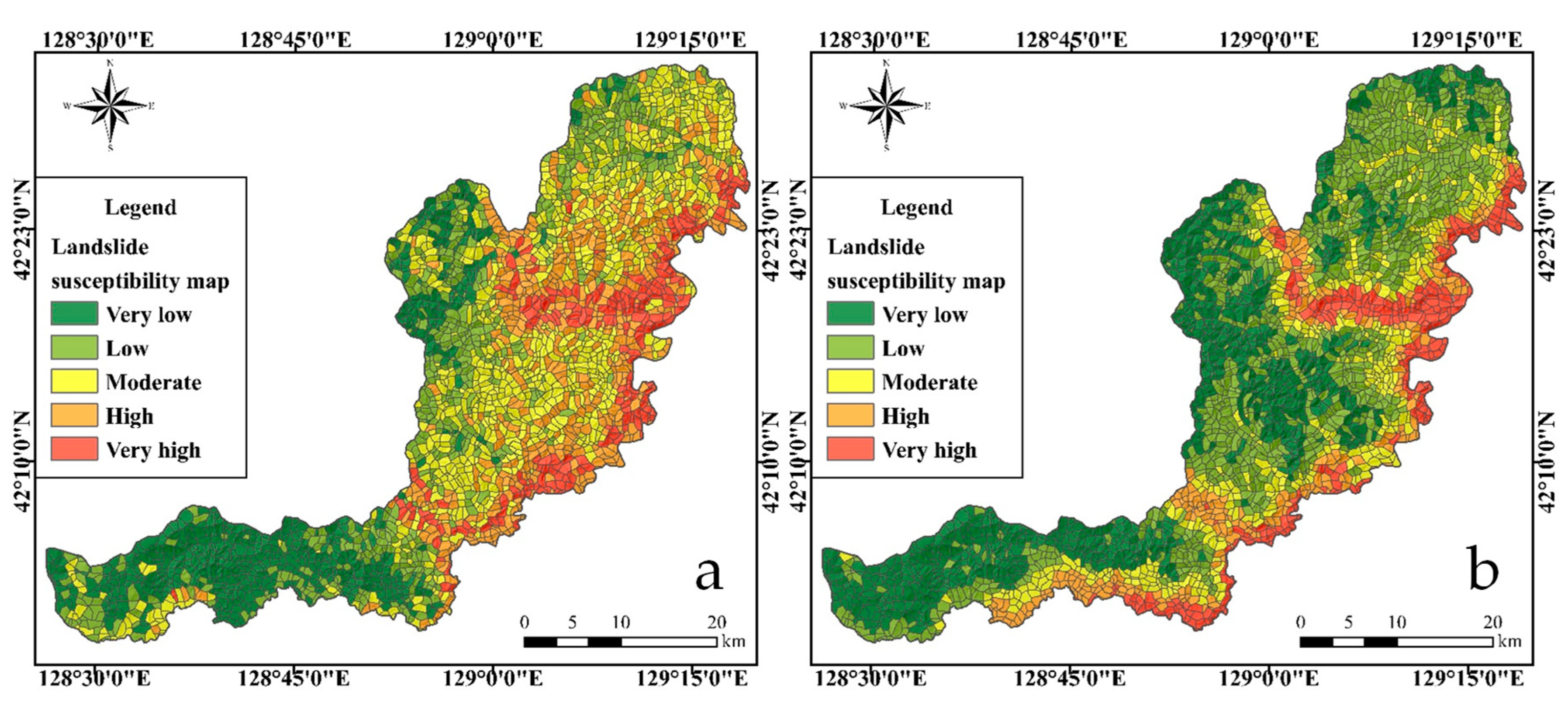
By comparing the five statistical parameters and AUC values of the two models, the SVM model was determined to be the optimal model. Therefore, the SVM model was used in this study to produce the landslide susceptibility map of the study area. The final model was established using the model with high accuracy and AUC value in the process of five-fold cross-validation. The natural breaks method was used to divide the landslide susceptibility of the study area into five grades: Very low, low, moderate, high, and very high. The landslide susceptibility map of the study area is shown in Figure 11.
Figure 11 and Table 3 show that the areas of the five susceptibility classes for the ANN model (very high, high, moderate, low, and very low) were 146.24, 297.95, 423.33, 310.44, and 297.95 km2, respectively. For landslide occurrence, the number of landslides in the five susceptibility classes were 43, 18, 10, 6, and 6, respectively. For the SVM model, the areas of the five susceptibility classes were 127.43, 151.60, 198.77, 491.19, and 506.91 km2, respectively. For landslide occurrence, the number of landslides in the five susceptibility classes were 52, 14, 8, 4, and 5, respectively.
5. Discussion
5.1. Slope Unit Classification Results
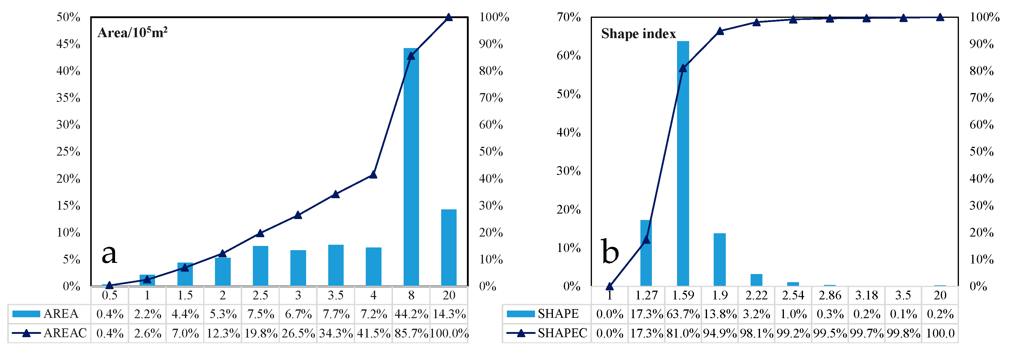
To evaluate the effect of dividing slope units, the area and shape indices of slope units were statistically analyzed. The ramp unit was used to extract the various influences, so the area it covers should be approximately the same size overall. The uniformity of slope unit area can be reflected by the distribution of slope unit area. It can be seen, from Figure 12a, that the slope unit area was concentrated between 4 and 8 × 10⁵ m2, accounting for 44.2% for the total number of slope units. If the slope unit is too flat, or there is an elongated unit, the uniformity inside the unit will be destroyed to a great extent. The shape index can be used to evaluate the shape of the slope unit. The shape index of the slope units can be calculated using the following equation:
where S is the shape index, L is the perimeter of the slope units, and A is the area of the slope units. According to the definition of the shape index, the shape index of a circle is 1, that of a square is 1.27, and that of an equilateral triangle is 1.59. Based on Figure 12b, the slope units with shape index below 1.59 accounted for 81.0%, which means that most of the slope units were between circle and equilateral triangle shapes; however, there were a few elongated slope units. Thus, the effect of dividing slope units was reasonable.
In addition, in the process of dividing slope units, it was found that compared with the hydrologic subdivision method, there is no large amount of parallel river network in the process of dividing slope units by the curvature watershed method. Moreover, the number of unreasonable units generated is much less than the hydrologic analysis method, so the later manual modification work is much less.
5.2. Comparison between ANN and SVM Model
Landslide susceptibility mapping is a popular research issue due to its non-linear characteristics. Although many mathematical methods have been applied to landslide susceptibility mapping, the prediction accuracy of these models is not very stable. Therefore, the same model cannot be applied to all studies. As a result, one of the key problems in landslide susceptibility mapping is to find a landslide susceptibility model which is suitable for a specific study area. In this study, the ANN and SVM models were introduced to establish a landslide susceptibility model for the area southeast of Helong city.
Through the training and testing of the two selected models, a confusion matrix was obtained, and the corresponding statistical parameters of each model were calculated to evaluate their respective advantages and disadvantages. From Table 2, the mean AUC values of ANN and SVM models differ greatly: in the training stage they were 88.60% and 93.22%, respectively; in the testing stage they were 84.52% and 89.74%, respectively. The AUC values of the two models decreased in the testing stage (by 4.08% for the ANN model and 3.48% for the SVM model), and that of the ANN model decreased significantly. According to the mean AUC value, the SVM model was slightly better than the ANN model (4.62% for the training stage, 5.22% for the testing stage). For the standard deviation of the AUC value in the training stage, that of the ANN model was obviously larger than that of the SVM model (2.48% for the ANN model, 0.83% for the SVM model). This indicated that the stability of the SVM model was better than that of ANN model in the training stage. In the testing stage, for the ANN model, the standard deviation of the AUC value (2.88%) increased slightly, and similarly for the SVM model (1.50%); however, the SVM model was more stable. From the mean AUC value alone, we believe that the SVM model could be the best.
For the statistical parameters, in the training stage, the mean accuracies were 83.27% and 88.56%, respectively, for the ANN model and the SVM model; in the testing stage, these were 71.23% and 84.30%. The standard deviation of the accuracy, in the training stage, was 6.11% and 1.71%, respectively, for the ANN model and the SVM model; in the testing stage, these were 1.75% and 2.72%. In terms of accuracy, the SVM model performed better than the ANN model (5.29% for training stage, 13.07% for testing stage). In terms of stability (according to accuracy) in the training stage, the SVM model was better than the ANN model (4.40%); however, in the testing stage, the ANN model was better than the SVM model (0.97%). From the aspect of mean accuracy, the SVM model was superior to the ANN model in both prediction accuracy and stability.
For the other four statistical parameters, the stability of the two models declined in the testing stage. In particular, the stability of the positive predictive value and negative positive value of the ANN model decreased greatly, which means the accuracy of the ANN model in predicting landslide units and non-landslide units is very unstable. The mean values of the four statistical parameters of the two models declined, but the ANN model showed a large drop (more than 10%). From the aspect of these four statistical parameters, the SVM model could also be considered as the optimal model.
5.3. Comparison with Other Models
In the evaluation of related geological disasters in Helong city, we used the information content method (ICM) and analytic hierarchy process (AHP) to evaluate the landslide susceptibility of the whole of Helong city based on both the grid unit and slope unit; the results are shown in Table 4 First, from the perspective of different mapping units, it can be seen that when ICM and AHP use grid units and slope units, respectively, for the landslide susceptibility evaluation of Helong city, their prediction accuracy is quite different. The prediction accuracy of the slope unit is obviously higher than that of the grid unit. This shows that it is reasonable to use the slope unit as the mapping unit of landslide susceptibility in this paper. Furthermore, the prediction accuracy of the two models established in this paper is higher than that of ICM and AHP models. In particular, the prediction accuracy of SVM model is the highest. This is because landslide susceptibility mapping is a dichotomous problem, and the SVM model is better for making predictions in such problems.
5.4. Landslide Suceptibility Map analysis
The landslide susceptibility map should meet the following two requirements [37]:
(1) The landslide points should be distributed in the areas with high susceptibility as much as possible. The purpose of this is to evaluate the accuracy of grading the sensitivity of landslides.
(2) In the landslide susceptibility map, the points predicted to be of high susceptibility should account for as low a proportion as possible. The purpose of this is to reduce the redundancy of high landslide susceptibility prediction and improve the hit ratio of susceptibility assessment.
Table 3 shows that the very high and high susceptibility areas for SVM model had a combined area of 279.03 km2, accounting for 18.90% of the total study area. Regarding the landslide occurrence, the very high and high susceptibility areas had 66 landslides, accounting for 79.52% of the total landslides. For the ANN model, the very high and high susceptibility areas had a combined area of 444.19 km2, accounting for 30.01% of the total study area. Regarding the landslide occurrence, the very high and high susceptibility areas had 61 landslides, accounting for 70.49% of the total landslides. This shows that the landslide susceptibility map produced by the SVM model in this paper is more reasonable than that of the ANN model.
According to Figure 11, the very high, high, and moderate susceptibility areas were mainly distributed along rivers. The reason for this is that the erosion caused by a river increases the slope angle along the river. To adapt to the erosion of the river, landslides and other disasters often occur along rivers, thus reducing the slope angle adjacent to the river. Furthermore, for slopes located close to a river, the slope foot is soaked by the river water, which reduces the strength of the rock and soil mass inside, thus leading to landslides. The low susceptibility area was mainly distributed in the northwest of the study area. In this area, the vegetation coverage is high and human engineering activities are weak; thus, the geological environment of this area is relatively stable, and landslides are less common.
6. Conclusions
In this study, we produced a landslide susceptibility map of the area to the southeast of Helong city. A total of 83 landslides were mapped in the study area through remote sensing interpretation and field investigation. The slope unit divided by the curvature watershed method was selected as the mapping unit. Based on field investigations and previous studies, three groups of influencing factors—lithological factors, topographic factors, and geological environment factors (a total of ten influencing factors: lithology, elevation, slope angle, slope aspect, topographic relief, curvature, land use, rainfall, distance to river, and distance to faults)—were selected to establish landslide susceptibility models. The ANN and SVM methods were used to build the models. Five-fold cross-validation, the ROC curve, and statistical parameters were used to optimize the models. Finally, the landslide susceptibility map was classified into five classes—very high, high, moderate, low, and very low.
According to the model fitting results, the SVM model was the optimal model for our purposes. For the five classes—very high, high, moderate, low, and very low—the areas of the grades from the SVM model were 127.43, 151.60, 198.77, 491.19, and 506.91 km2, respectively. For landslide occurrence, the number of landslides in the five susceptibility classes were 52, 14, 8, 4, and 5, respectively; therefore, the very high and high susceptibility areas included 79.52% of the total landslides. This indicates that the landslide susceptibility map produced in this paper is reasonable.
In conclusion, the following inferences were obtained:
(1) Because the slope units are more closely related to the real topographic and geomorphic features, the obtained landslide susceptibility map is more reasonable. Thus, it is suggested that the slope unit should be used as the mapping unit in related work.
(2) The SVM model needs less data and is more suitable for binary classification, so it can be given priority in the study of landslide susceptibility mapping.
Author Contributions
C.Y. contributed to data analysis and manuscript writing. J.C. proposed the main structure of this study. All authors have read and agreed to the published version of the manuscript.
Funding
This research was funded by the Natural Science Foundations of China grant number [U1702241].
Acknowledgments
Thanks to anonymous reviewers for their valuable feedback on the manuscript.
Conflicts of Interest
The authors declare no conflict of interest.
Appendix A

Table A1.
Description of the Landslides.
| No. | Lithology | Slope Angle | Slope Aspect | Slope Height | Slope Shape | Microrelief | Landslide Scale | Failure Mode |
|---|---|---|---|---|---|---|---|---|
| 1 | Granodiorite | 60 | 198 | 6 | Convex | Steep Slope | Small | Pull-Type |
| 2 | Granodiorite | 79 | 162 | 17 | Convex | Steep Coast | Middle | Pull-Type |
| 3 | Granodiorite | 63 | 162 | 24 | Convex | Steep Coast | Small | Toppling |
| 4 | Monzonitic Granite | 65 | 50 | 20 | Concave | Steep Coast | Middle | Pull-Type |
| 5 | Monzonitic Granite | 71 | 45 | 11 | Convex | Steep Coast | Small | Pull-Type |
| 6 | Granodiorite | 52 | 215 | 24 | Convex | Steep Slope | Small | Sliding |
| 7 | Granodiorite | 57 | 110 | 15 | Concave | Steep Slope | Middle | Pull-Type |
| 8 | Monzonitic Granite | 69 | 148 | 17 | Convex | Steep Coast | Small | Pull-Type |
| 9 | Monzonitic Granite | 62 | 221 | 17 | Convex | Steep Coast | Small | Sliding |
| 10 | Dioritic Porphyrite | 52 | 275 | 12 | Convex | Steep Slope | Small | Pull-Type |
| 11 | Basalt | 81 | 178 | 50 | Convex | Steep Coast | Middle | Toppling |
| 12 | Basalt | 86 | 202 | 42 | Convex | Steep Coast | Middle | Pull-Type |
| 13 | Basalt | 75 | 105 | 17 | Convex | Steep Coast | Small | Sliding |
| 14 | Basalt | 58 | 128 | 23 | Concave | Steep Slope | Middle | Pull-Type |
| 15 | Basalt | 87 | 178 | 32 | Convex | Steep Coast | Middle | Pull-Type |
| 16 | Basalt | 82 | 130 | 20 | Concave | Steep Coast | Middle | Pull-Type |
| 17 | Basalt | 68 | 178 | 18 | Convex | Steep Coast | Small | Sliding |
| 18 | Basalt | 40 | 270 | 25 | Straight | Steep Slope | Small | Pull-Type |
| 19 | Basalt | 84 | 253 | 12 | Convex | Steep Coast | Small | Pull-Type |
| 20 | Basalt | 86 | 280 | 25 | Convex | Steep Coast | Middle | Pull-Type |
| 21 | Basalt | 84 | 183 | 20 | Convex | Steep Coast | Middle | Pull-Type |
| 22 | Basalt | 81 | 210 | 12 | Concave | Steep Coast | Small | Pull-Type |
| 23 | Granodiorite | 71 | 193 | 23 | Convex | Steep Coast | Small | Pull-Type |
| 24 | Granodiorite | 37 | 195 | 49 | Convex | Steep Slope | Small | Pull-Type |
| 25 | Granodiorite | 40 | 196 | 43 | Convex | Steep Slope | Small | Toppling |
| 26 | Granodiorite | 38 | 154 | 25 | Concave | Steep Slope | Small | Pull-Type |
| 27 | Granodiorite | 42 | 268 | 9 | Straight | Steep Slope | Middle | Pull-Type |
| 28 | Granodiorite | 55 | 254 | 8 | Concave | Steep Slope | Small | Pull-Type |
| 29 | Monzonitic Granite | 43 | 190 | 12 | Straight | Steep Slope | Small | Pull-Type |
| 30 | Granite | 41 | 230 | 11 | Convex | Steep Slope | Middle | Pull-Type |
| 31 | Monzonitic Granite | 62 | 130 | 10 | Convex | Steep Coast | Small | Pull-Type |
| 32 | Basalt | 87 | 250 | 12 | Concave | Steep Coast | Small | Pull-Type |
| 33 | Diorite | 71 | 155 | 10 | Convex | Steep Coast | Small | Pull-Type |
| 34 | Granodiorite | 42 | 136 | 8 | Convex | Steep Slope | Small | Pull-Type |
| 35 | Granodiorite | 55 | 152 | 5 | Convex | Steep Slope | Small | Pull-Type |
| 36 | Basalt | 50 | 135 | 14 | Straight | Steep Slope | Small | Pull-type |
| 37 | Granodiorite | 71 | 90 | 9 | Convex | Steep Coast | Small | Toppling |
| 38 | Monzonitic Granite | 35 | 186 | 15 | Convex | Steep Slope | Small | Pull-Type |
| 39 | Monzonitic Granite | 36 | 135 | 30 | Straight | Steep Slope | Small | Pull-Type |
| 40 | Diorite | 37 | 174 | 50 | Straight | Steep Slope | Small | Toppling |
| 41 | Granodiorite | 48 | 148 | 16 | Convex | Steep Slope | Small | Pull-Type |
| 42 | Granodiorite | 85 | 128 | 12 | Convex | Steep Coast | Small | Toppling |
| 43 | Granodiorite | 77 | 224 | 15 | Convex | Steep Coast | Small | Toppling |
| 44 | Granodiorite | 67 | 188 | 77 | Convex | Steep Coast | Middle | Sliding |
| 45 | Monzonitic Granite | 57 | 204 | 61 | Concave | Steep Slope | Middle | Staggered Breaking |
| 46 | Monzonitic Granite | 81 | 228 | 25 | Convex | Steep Coast | Middle | Toppling |
| 47 | Monzonitic Granite | 72 | 250 | 52 | Convex | Steep Coast | Middle | Toppling |
| 48 | Monzonitic Granite | 72 | 185 | 31 | Concave | Steep Coast | Middle | Toppling |
| 49 | Monzonitic Granite | 76 | 190 | 142 | Convex | Steep Coast | Middle | Toppling |
| 50 | Monzonitic Granite | 74 | 120 | 13 | Convex | Steep Coast | Small | Toppling |
| 51 | Monzonitic Granite | 69 | 204 | 108 | Convex | Steep Coast | Large | Pull-Splitting |
| 52 | Diorite | 78 | 172 | 160 | Convex | Steep Coast | Large | Toppling |
| 53 | Diorite | 62 | 134 | 224 | Convex | Steep Coast | Large | Toppling |
| 54 | Granodiorite | 68 | 24 | 23 | Convex | Steep Coast | Middle | Toppling |
| 55 | Granodiorite | 65 | 150 | 136 | Concave | Steep Coast | Large | Sliding |
| 56 | Granodiorite | 76 | 162 | 228 | Convex | Steep Coast | Large | Pull-Splitting |
| 57 | Monzonitic Granite | 70 | 155 | 151 | Concave | Steep Coast | Large | Staggered Breaking |
| 58 | Monzonitic Granite | 51 | 155 | 32 | Convex | Steep Slope | Small | Toppling |
| 59 | Granodiorite | 70 | 72 | 32 | Straight | Steep Coast | Small | Pull-Splitting |
| 60 | Basalt | 72 | 125 | 46 | Convex | Steep Coast | Middle | Toppling |
| 61 | Basalt | 58 | 200 | 45 | Convex | Steep Slope | Middle | Toppling |
| 62 | Basalt | 83 | 218 | 28 | Convex | Steep Coast | Small | Toppling |
| 63 | Basalt | 60 | 152 | 89 | Concave | Steep Slope | Middle | Sliding |
| 64 | Basalt | 52 | 105 | 7 | Convex | Steep Slope | Small | Pull-Splitting |
| 65 | Granodiorite | 60 | 130 | 23 | Convex | Steep Slope | Small | Pull-Splitting |
| 66 | Andesite | 38 | 220 | 65 | Convex | Steep Slope | Middle | Pull-Splitting |
| 67 | Andesite | 50 | 245 | 55 | Concave | Steep Slope | Middle | Pull-Splitting |
| 68 | Andesite | 70 | 135 | 15 | Straight | Steep Coast | Small | Sliding |
| 69 | Monzonitic Granite | 44 | 215 | 12 | Concave | Steep Slope | Small | Toppling |
| 70 | Granodiorite | 70 | 190 | 24 | Straight | Steep Coast | Small | Toppling |
| 71 | Granite | 53 | 170 | 14 | Convex | Steep Coast | Small | Pull-Splitting |
| 72 | Quartzite | 73 | 130 | 40 | Convex | Steep Coast | Small | Pull-Splitting |
| 73 | Quartzite | 72 | 184 | 42 | Concave | Steep Coast | Small | Staggered Breaking |
| 74 | Quartzite | 52 | 154 | 50 | Convex | Steep Slope | Small | Staggered Breaking |
| 75 | Quartzite | 70 | 192 | 45 | Convex | Steep Coast | Middle | Staggered Breaking |
| 76 | Monzonitic Granite | 58 | 195 | 55 | Convex | Steep Slope | Middle | Staggered Breaking |
| 77 | Granodiorite | 80 | 56 | 8 | Straight | Steep Coast | Small | Pull-Splitting |
| 78 | Monzonitic Granite | 71 | 170 | 75 | Convex | Steep Coast | Small | Toppling |
| 79 | Monzonitic Granite | 75 | 138 | 40 | Convex | Steep Coast | Small | Toppling |
| 80 | Monzonitic Granite | 51 | 85 | 15 | Straight | Steep Slope | Small | Toppling |
| 81 | Granodiorite | 68 | 175 | 7 | Straight | Steep Coast | Small | Toppling |
| 82 | Basalt | 62 | 184 | 7 | Convex | Steep Coast | Small | Toppling |
| 83 | Granodiorite | 40 | 160 | 19 | Convex | Steep Slope | Small | Pull-Splitting |
Note: Landslide scale: (a) Small; Landslide volume <1 × 10⁴ m3; (b) Middle: 100 × 104 m3 < Landslide volume <104 m3.
References
- Cao, C.; Wang, Q.; Chen, J.; Ruan, Y.; Zheng, L.; Song, S.; Niu, C. Landslide susceptibility mapping in vertical distribution law of precipitation area: Case of the xulong hydropower station reservoir, southwestern China. Water 2016, 8, 270. [Google Scholar] [CrossRef] [Green Version]
- Sun, X.; Chen, J.; Bao, Y.; Han, X.; Zhan, J.; Peng, W. Landslide susceptibility mapping using logistic regression analysis along the jinsha river and its tributaries close to derong and deqin county, southwestern China. ISPRS Int. J. Geo-Inf. 2018, 7, 438. [Google Scholar] [CrossRef] [Green Version]
- Zhan, J.; Chen, J.; Zhang, W.; Han, X.; Sun, X.; Bao, Y. Mass movements along a rapidly uplifting river valley: An example from the upper Jinsha River, southeast margin of the Tibetan Plateau. Environ. Earth Sci. 2018, 77, 634. [Google Scholar] [CrossRef]
- Wang, F.; Xu, P.; Wang, C.; Wang, N.; Jiang, N. Application of a GIS-Based slope Unit Method for landslide susceptibility mapping along the Longzi River, Southeastern Tibetan Plateau, China. ISPRS Int. J. Geo-Inf. 2017, 6, 172. [Google Scholar] [CrossRef] [Green Version]
- Hearn, G.J.; Hart, A.B. Landslide susceptibility mapping: A practitioner’s view. Bull. Eng. Geol. Environ. 2019, 78, 5811–5826. [Google Scholar] [CrossRef]
- Reichenbach, P.; Rossi, M.; Malamud, B.D.; Mihir, M.; Guzzetti, F. A review of statistically-based landslide susceptibility models. Earth-Sci. Rev. 2018, 180, 60–91. [Google Scholar] [CrossRef]
- Guzzetti, F.; Mondini, A.C.; Cardinali, M.; Fiorucci, F.; Santangelo, M.; Chang, K.T. Landslide inventory maps: New tools for an old problem. Earth-Sci. Rev. 2012, 112, 42–66. [Google Scholar] [CrossRef] [Green Version]
- Yang, X.J.; Chen, L.D. Geoinformation. Using multi-temporal remote sensor imagery to detect earthquake-triggered landslides. Int. J. Appl. Earth Obs. Geoinf. 2010, 12, 487–495. [Google Scholar] [CrossRef]
- Mulas, M.; Corsini, A.; Cuozzo, G.; Callegari, M.; Thiebes, B.; Mair, V. Quantitative Monitoring of Surface Movements on Active Landslides by Multi-Temporal, High-Resolution X-Band SAR Amplitude Information: Preliminary Results; CRC Press: Boca Raton, FL, USA, 2016; pp. 1511–1516. [Google Scholar]
- Schlogel, R.; Marchesini, I.; Alvioli, M.; Reichenbach, P.; Rossi, M.; Malet, J.P. Optimizing landslide susceptibility zonation: Effects of DEM spatial resolution and slope unit delineation on logistic regression models. Geomorphology 2018, 301, 10–20. [Google Scholar] [CrossRef]
- Rotigliano, E.; Cappadonia, C.; Conoscenti, C.; Costanzo, D.; Agnesi, V. Slope units-based flow susceptibility model: Using validation tests to select controlling factors. Nat. Hazards 2012, 61, 143–153. [Google Scholar] [CrossRef]
- Alvioli, M.; Marchesini, I.; Reichenbach, P.; Rossi, M.; Ardizzone, F.; Fiorucci, F.; Guzzetti, F. Automatic delineation of geomorphological slope units with r.slopeunits v1.0 and their optimization for landslide susceptibility modeling. Geosci. Model Dev. 2016, 9, 3975–3991. [Google Scholar] [CrossRef] [Green Version]
- Pourghasemi, H.R.; Rossi, M. Landslide susceptibility modeling in a landslide prone area in Mazandarn Province, north of Iran: A comparison between GLM, GAM, MARS, and M-AHP methods. Theor. Appl. Climatol. 2017, 130, 609–633. [Google Scholar] [CrossRef]
- Lagomarsino, D.; Tofani, V.; Segoni, S.; Catani, F.; Casagli, N. A Tool for Classification and Regression Using Random Forest Methodology: Applications to Landslide Susceptibility Mapping and Soil Thickness Modeling. Environ. Model. Assess. 2017, 22, 201–214. [Google Scholar] [CrossRef]
- Dou, J.; Bui, D.T.; Yunus, A.P.; Jia, K.; Song, X.; Revhaug, I.; Xia, H.; Zhu, Z. Optimization of Causative Factors for Landslide Susceptibility Evaluation Using Remote Sensing and GIS Data in Parts of Niigata, Japan. PLoS ONE 2015, 10, e0133262. [Google Scholar] [CrossRef] [Green Version]
- Frattini, P.; Crosta, G.; Carrara, A. Techniques for evaluating the performance of landslide susceptibility models. Eng. Geol. 2010, 111, 62–72. [Google Scholar] [CrossRef]
- Chen, W.; Li, W.; Chai, H.; Hou, E.; Li, X.; Ding, X. GIS-based landslide susceptibility mapping using analytical hierarchy process (AHP) and certainty factor (CF) models for the Baozhong region of Baoji City, China. Environ. Earth Sci. 2016, 75, 63. [Google Scholar] [CrossRef]
- Cao, C.; Xu, P.; Wang, Y.; Chen, J.; Zheng, L.; Niu, C. Flash Flood Hazard Susceptibility Mapping Using Frequency Ratio and Statistical Index Methods in Coalmine Subsidence Areas. Sustainability 2016, 8, 948. [Google Scholar] [CrossRef] [Green Version]
- Xiao, T.; Segoni, S.; Chen, L.; Yin, K.; Casagli, N. A step beyond landslide susceptibility maps: A simple method to investigate and explain the different outcomes obtained by different approaches. Landslides 2020, 17, 627–640. [Google Scholar] [CrossRef] [Green Version]
- Bai, S.-B.; Wang, J.; Lue, G.-N.; Zhou, P.-G.; Hou, S.-S.; Xu, S.-N. GIS-based logistic regression for landslide susceptibility mapping of the Zhongxian segment in the Three Gorges area, China. Geomorphology 2010, 115, 23–31. [Google Scholar] [CrossRef]
- Sun, X.; Chen, J.; Han, X.; Bao, Y.; Zhan, J.; Peng, W. Application of a GIS-based slope unit method for landslide susceptibility mapping along the rapidly uplifting section of the upper Jinsha River, South-Western China. Bull. Eng. Geol. Environ. 2019. [Google Scholar] [CrossRef]
- Segoni, S.; Pappafico, G.; Luti, T.; Catani, F. Landslide susceptibility assessment in complex geological settings: Sensitivity to geological information and insights on its parameterization. Landslides 2020. [Google Scholar] [CrossRef] [Green Version]
- Ren, D.; Zhou, D.; Liu, D.; Dong, F.; Ma, S.; Huang, H. Formation mechanism of the Upper Triassic Yanchang Formation tight sandstone reservoir in Ordos Basin-Take Chang 6 reservoir in Jiyuan oil field as an example. J. Pet. Sci. Eng. 2019, 178, 497–505. [Google Scholar] [CrossRef]
- Ayalew, L.; Yamagishi, H. The application of GIS-based logistic regression for landslide susceptibility mapping in the Kakuda-Yahiko Mountains, Central Japan. Geomorphology 2005, 65, 15–31. [Google Scholar] [CrossRef]
- Lee, S.; Min, K. Statistical analysis of landslide susceptibility at Yongin, Korea. Environ. Geol. 2001, 40, 1095–1113. [Google Scholar] [CrossRef]
- Conforti, M.; Pascale, S.; Robustelli, G.; Sdao, F. Evaluation of prediction capability of the artificial neural networks for mapping landslide susceptibility in the Turbolo River catchment (northern Calabria, Italy). Catena 2014, 113, 236–250. [Google Scholar] [CrossRef]
- Oh, H.-J.; Pradhan, B. Application of a neuro-fuzzy model to landslide-susceptibility mapping for shallow landslides in a tropical hilly area. Comput. Geosci. 2011, 37, 1264–1276. [Google Scholar] [CrossRef]
- Park, S.; Choi, C.; Kim, B.; Kim, J. Landslide susceptibility mapping using frequency ratio, analytic hierarchy process, logistic regression, and artificial neural network methods at the Inje area, Korea. Environ. Earth Sci. 2013, 68, 1443–1464. [Google Scholar] [CrossRef]
- Hong, H.; Pradhan, B.; Xu, C.; Tien Bui, D. Spatial prediction of landslide hazard at the Yihuang area (China) using two-class kernel logistic regression, alternating decision tree and support vector machines. Catena 2015, 133, 266–281. [Google Scholar] [CrossRef]
- Binh Thai, P.; Dieu Tien, B.; Dholakia, M.B.; Prakash, I.; Ha Viet, P.; Mehmood, K.; Hung Quoc, L. A novel ensemble classifier of rotation forest and Naive Bayer for landslide susceptibility assessment at the Luc Yen district, Yen Bai Province (Viet Nam) using GIS. Geomat. Nat. Hazards Risk 2017, 8, 649–671. [Google Scholar] [CrossRef] [Green Version]
- Chen, W.; Xie, X.; Wang, J.; Pradhan, B.; Hong, H.; Bui, D.T.; Duan, Z.; Ma, J. A comparative study of logistic model tree, random forest, and classification and regression tree models for spatial prediction of landslide susceptibility. Catena 2017, 151, 147–160. [Google Scholar] [CrossRef] [Green Version]
- Dieu Tien, B.; Tran Anh, T.; Klempe, H.; Pradhan, B.; Revhaug, I. Spatial prediction models for shallow landslide hazards: A comparative assessment of the efficacy of support vector machines, artificial neural networks, kernel logistic regression, and logistic model tree. Landslides 2016, 13, 361–378. [Google Scholar] [CrossRef]
- Kumar, D.; Thakur, M.; Dubey, C.S.; Shukla, D.P. Landslide Susceptibility Mapping & Prediction using Support Vector Machine for Mandakini River Basin, Garhwal Himalaya, India. Geomorphology 2017, 295, 115–125. [Google Scholar]
- Chen, W.; Pourghasemi, H.R.; Kornejady, A.; Zhang, N. Landslide spatial modeling: Introducing new ensembles of ANN, MaxEnt, and SVM machine learning techniques. Geoderma 2017, 305, 314–327. [Google Scholar] [CrossRef]
- Yesilnacar, E.; Topal, T. Landslide susceptibility mapping: A comparison of logistic regression and neural networks methods in a medium scale study, Hendek region (Turkey). Eng. Geol. 2005, 79, 251–266. [Google Scholar] [CrossRef]
- Binh Thai, P.; Dieu Tien, B.; Prakash, I.; Dholakia, M.B. Hybrid integration of Multilayer Perceptron Neural Networks and machine learning ensembles for landslide susceptibility assessment at Himalayan area (India) using GIS. Catena 2017, 149, 52–63. [Google Scholar] [CrossRef]
- Su, Q.; Zhang, J.; Zhao, S.; Wang, L.; Liu, J.; Guo, J. Comparative Assessment of Three Nonlinear Approaches for Landslide Susceptibility Mapping in a Coal Mine Area. ISPRS Int. J. Geo-Inf. 2017, 6, 228. [Google Scholar] [CrossRef] [Green Version]
- Aditian, A.; Kubota, T.; Shinohara, Y. Comparison of GIS-based landslide susceptibility models using frequency ratio, logistic regression, and artificial neural network in a tertiary region of Ambon, Indonesia. Geomorphology 2018, 318, 101–111. [Google Scholar] [CrossRef]
- Jiang, P.; Zeng, Z.; Chen, J.; Huang, T. Generalized Regression Neural Networks with K-Fold Cross-Validation for Displacement of Landslide Forecasting. In Advances in Neural Networks—Isnn 2014; Zeng, Z., Li, Y., King, I., Eds.; Springer: Cham, Switzerland, 2014; Volume 8866, pp. 533–541. [Google Scholar]
- Jiang, T.; Lei, P.; Qin, Q. An Application of SVM-Based Classification in Landslide Stability. Intell. Autom. Soft Comput. 2016, 22, 267–271. [Google Scholar] [CrossRef]
- Li, X.Z.; Kong, J.M.J.N.H.; Sciences, E.S. Application of GA-SVM method with parameter optimization for landslide development prediction. Nat. Hazards Earth Syst. Sci. 2014, 14, 5295–5322. [Google Scholar] [CrossRef] [Green Version]
- Pradhan, B.; Sameen, M.I. Manifestation of SVM-Based Rectified Linear Unit (ReLU) Kernel Function in Landslide Modelling; Springer: Singapore, 2018. [Google Scholar]
- San, B.T. An evaluation of SVM using polygon-based random sampling in landslide susceptibility mapping: The Candir catchment area (western Antalya, Turkey). Int. J. Appl. Earth Obs. Geoinf. 2014, 26, 399–412. [Google Scholar] [CrossRef]
- Ballabio, C.; Sterlacchini, S. Support Vector Machines for Landslide Susceptibility Mapping: The Staffora River Basin Case Study, Italy. Math. Geosci. 2012, 44, 47–70. [Google Scholar] [CrossRef]
- Chen, W.; Pourghasemi, H.R.; Panahi, M.; Kornejady, A.; Wang, J.; Xie, X.; Cao, S. Spatial prediction of landslide susceptibility using an adaptive neuro-fuzzy inference system combined with frequency ratio, generalized additive model, and support vector machine techniques. Geomorphology 2017, 297, 69–85. [Google Scholar] [CrossRef]
- Zhang, X.; Wang, Q.; Huo, Z.; Yu, T.; Wang, G.; Liu, T.; Wang, W. Prediction of Frost-Heaving Behavior of Saline Soil in Western Jilin Province, China, by Neural Network Methods. Math. Probl. Eng. 2017. [Google Scholar] [CrossRef] [Green Version]
- Hong, H.; Pradhan, B.; Jebur, M.N.; Bui, D.T.; Xu, C.; Akgun, A. Spatial prediction of landslide hazard at the Luxi area (China) using support vector machines. Environ. Earth Sci. 2016, 75. [Google Scholar] [CrossRef]
- Huang, F.; Yin, K.; Huang, J.; Gui, L.; Wang, P. Landslide susceptibility mapping based on self-organizing-map network and extreme learning machine. Eng. Geol. 2017, 223, 11–22. [Google Scholar] [CrossRef]
Figure 1.
Geographical position and landslide inventory of the study area. (a,b): geographical position of the study area; (c) landslide inventory of the study area; (d) geological map of the study area; (e,f) typical landslides of the study area.
Figure 1.
Geographical position and landslide inventory of the study area. (a,b): geographical position of the study area; (c) landslide inventory of the study area; (d) geological map of the study area; (e,f) typical landslides of the study area.

Figure 2.
Flowchart of this study.

Figure 3.
Construction process of the slope units based on the curvature watershed method.

Figure 4.
(a) Elevation map; (b) slope angle map.

Figure 5.
Influencing factor maps of the study area: (a) lithology (downloaded using 91 Weitu software), (b) elevation, (c) slope angle, and (d) slope aspect.
Figure 5.
Influencing factor maps of the study area: (a) lithology (downloaded using 91 Weitu software), (b) elevation, (c) slope angle, and (d) slope aspect.

Figure 6.
Influencing factors maps of the study area: (a) topographic relief, (b) curvature, (c) land-use, and (d) rainfall.
Figure 6.
Influencing factors maps of the study area: (a) topographic relief, (b) curvature, (c) land-use, and (d) rainfall.

Figure 7.
Influencing factors maps of the study area: (a) distance to river and (b) distance to fault.
Figure 7.
Influencing factors maps of the study area: (a) distance to river and (b) distance to fault.

Figure 8.
Schematic diagram of a simple artificial neural network (ANN) model.

Figure 9.
Division of slope units of the study area.

Figure 10.
Area under the curve (AUC) values of model evaluation parameters when the hidden neurons of ANN model varied.
Figure 10.
Area under the curve (AUC) values of model evaluation parameters when the hidden neurons of ANN model varied.

Figure 11.
Landslide susceptibility map. (a) ANN model; and (b) support vector machine (SVM) model.

Figure 12.
Statistics of morphological characteristics of slope units. (a) Slope unit area distribution diagram; (b) slope unit shape index distribution diagram.
Figure 12.
Statistics of morphological characteristics of slope units. (a) Slope unit area distribution diagram; (b) slope unit shape index distribution diagram.

Table 1.
Description of the Lithology.
| System | Code | Lithology |
|---|---|---|
| Quaternary | Q | Alluvial–Diluvial, Gravel, Sub-Sandy Soil, Sub-Clay, and Basalt |
| Neogene | N | Sandstone, Conglomerate, and Siltstone with Basalt |
| Cretaceous | K | Sandstone, Conglomerate, Siltstone with Limestone, and Oil Limestone |
| Jurassic | J | Andesite and Tuff |
| Middle Proterozoic | Pt | Marble |
| New Archean | Ar | Black Cloud Amphibolic Granulite and Granulite |
Table 2.
Performance of the Two Slope-Unit-Fitted Landslide Susceptibility Models (%).
| Stage | Method | Statistical Index | K = 1 | K = 2 | K = 3 | K = 4 | K = 5 | Mean | Standard Deviation |
|---|---|---|---|---|---|---|---|---|---|
| Training | ANN | AUC | 88.20 | 91.10 | 90.30 | 84.70 | 88.70 | 88.60 | 2.48 |
| AC | 86.57 | 89.39 | 85.07 | 73.48 | 81.82 | 83.27 | 6.11 | ||
| SE | 91.53 | 90.63 | 83.10 | 72.46 | 82.81 | 84.11 | 7.68 | ||
| SP | 82.67 | 88.24 | 87.30 | 74.60 | 80.88 | 82.74 | 5.49 | ||
| PP | 80.60 | 87.88 | 88.06 | 75.76 | 80.30 | 82.52 | 5.33 | ||
| NP | 92.54 | 90.91 | 82.09 | 71.21 | 83.33 | 84.02 | 8.49 | ||
| SVM | AUC | 92.70 | 93.40 | 92.30 | 93.20 | 94.50 | 93.22 | 0.83 | |
| AC | 87.31 | 89.39 | 86.57 | 88.64 | 90.91 | 88.56 | 1.71 | ||
| SE | 89.06 | 91.94 | 87.69 | 90.48 | 93.55 | 90.54 | 2.31 | ||
| SP | 85.71 | 87.14 | 85.51 | 86.96 | 88.57 | 86.78 | 1.24 | ||
| PP | 85.07 | 86.36 | 85.07 | 86.36 | 87.88 | 86.15 | 1.16 | ||
| NP | 89.55 | 92.42 | 88.06 | 90.91 | 93.94 | 90.98 | 2.31 | ||
| Testing | ANN | AUC | 83.20 | 87.00 | 82.10 | 88.20 | 82.10 | 84.52 | 2.88 |
| AC | 71.88 | 70.59 | 68.75 | 71.43 | 73.53 | 71.23 | 1.75 | ||
| SE | 73.33 | 81.82 | 65.00 | 66.67 | 72.22 | 71.81 | 6.62 | ||
| SP | 70.59 | 65.22 | 75.00 | 78.57 | 75.00 | 72.88 | 5.13 | ||
| PP | 68.75 | 52.94 | 81.25 | 82.35 | 76.47 | 72.35 | 12.10 | ||
| NP | 75.00 | 88.24 | 56.25 | 64.71 | 70.59 | 70.96 | 11.94 | ||
| SVM | AUC | 88.70 | 89.60 | 91.20 | 91.30 | 87.90 | 89.74 | 1.50 | |
| AC | 81.25 | 88.24 | 84.38 | 85.29 | 82.35 | 84.30 | 2.72 | ||
| SE | 81.25 | 93.33 | 82.35 | 83.33 | 82.35 | 84.52 | 4.98 | ||
| SP | 81.25 | 84.21 | 86.67 | 87.50 | 82.35 | 84.40 | 2.69 | ||
| PP | 81.25 | 82.35 | 87.50 | 88.24 | 82.35 | 84.34 | 3.26 | ||
| NP | 81.25 | 94.12 | 81.25 | 82.35 | 82.35 | 84.26 | 5.54 |
Note: K is the number of cross validations.
Table 3.
Statistical Results of the Landslide Susceptibility Map.
| Model | Susceptibility | Landslide Occurred | Total Study Area | ||
|---|---|---|---|---|---|
| Count | Ratio | Area (km2) | Ratio | ||
| ANN | Very Low | 6 | 7.23% | 297.95 | 20.19% |
| Low | 6 | 7.23% | 310.44 | 21.03% | |
| Moderate | 10 | 12.05% | 423.33 | 28.68% | |
| High | 18 | 21.69% | 297.95 | 20.19% | |
| Very High | 43 | 51.81% | 146.24 | 9.91% | |
| SVM | Very Low | 5 | 6.02% | 506.91 | 34.35% |
| Low | 4 | 4.82% | 491.19 | 33.28% | |
| Moderate | 8 | 9.64% | 198.77 | 13.47% | |
| High | 14 | 16.87% | 151.60 | 10.27% | |
| Very High | 52 | 62.65% | 127.43 | 8.63% | |
Table 4.
Modeling Fitting Results of the Study Area.
| Mapping Units | Method | Prediction Accuracy (Mean) | |
|---|---|---|---|
| Slope Units | ANN | Training | 89.72% |
| Validating | 88.08% | ||
| Slope Units | SVM | Training | 90.72% |
| Validating | 88.96% | ||
| Grid Units | ICM | - | 83.42% |
| Grid Units | AHP | - | 70.93% |
| Slope Units | ICM | - | 87.11% |
| Slope Units | AHP | - | 80.54% |
© 2020 by the authors. Licensee MDPI, Basel, Switzerland. This article is an open access article distributed under the terms and conditions of the Creative Commons Attribution (CC BY) license (http://creativecommons.org/licenses/by/4.0/).
Share and Cite
MDPI and ACS Style
Yu, C.; Chen, J. Landslide Susceptibility Mapping Using the Slope Unit for Southeastern Helong City, Jilin Province, China: A Comparison of ANN and SVM. Symmetry 2020, 12, 1047. https://0-doi-org.brum.beds.ac.uk/10.3390/sym12061047
AMA Style
Yu C, Chen J. Landslide Susceptibility Mapping Using the Slope Unit for Southeastern Helong City, Jilin Province, China: A Comparison of ANN and SVM. Symmetry. 2020; 12(6):1047. https://0-doi-org.brum.beds.ac.uk/10.3390/sym12061047
Chicago/Turabian StyleYu, Chenglong, and Jianping Chen. 2020. "Landslide Susceptibility Mapping Using the Slope Unit for Southeastern Helong City, Jilin Province, China: A Comparison of ANN and SVM" Symmetry 12, no. 6: 1047. https://0-doi-org.brum.beds.ac.uk/10.3390/sym12061047
Note that from the first issue of 2016, this journal uses article numbers instead of page numbers. See further details here.