Article

Engineering Graphics for Thermal Assessment: 3D Thermal Data Visualisation Based on Infrared Thermography, GIS and 3D Point Cloud Processing Software

by
Daniel Antón
1,2 and
José-Lázaro Amaro-Mellado
3,4,*
1
Research Group ‘TEP970: Innovación Tecnológica, Sistemas de Modelado 3D y Diagnosis Energética en Patrimonio y Edificación’, Departamento de Expresión Gráfica e Ingeniería en la Edificación, Escuela Técnica Superior de Ingeniería de Edificación, Universidad de Sevilla, 4A Reina Mercedes Avenue, 41012 Seville, Spain
2
The Creative and Virtual Technologies Research Laboratory, School of Architecture, Design and the Built Environment, Nottingham Trent University, 50 Shakespeare Street, Nottingham NG1 4FQ, UK
3
Departamento de Ingeniería Gráfica, Universidad de Sevilla, 41092 Seville, Spain
4
Instituto Geográfico Nacional—Servicio Regional en Andalucía, 41013 Seville, Spain
*
Author to whom correspondence should be addressed.
Submission received: 2 January 2021 / Revised: 11 February 2021 / Accepted: 16 February 2021 / Published: 18 February 2021
(This article belongs to the Special Issue Advances on Engineering Graphics: Improvements and New Proposals)

Abstract

:
Engineering graphics are present in the design stage, but also constitute a way to communicate, analyse, and synthesise. In the Architecture-Engineering-Construction sector, graphical data become essential in analysing buildings and constructions throughout their lifecycles, such as in the thermal behaviour assessment of building envelopes. Scientific research has addressed the thermal image mapping onto three-dimensional (3D) models for visualisation and analysis. However, the 3D point cloud data creation of buildings’ thermal behaviour directly from rectified infrared thermography (IRT) thermograms is yet to be investigated. Therefore, this paper develops an open-source software graphical method to produce 3D thermal data from IRT images for temperature visualisation and subsequent analysis. This low-cost approach uses both a geographic information system for the thermographic image rectification and the point clouds production, and 3D point cloud processing software. The methodology has been proven useful to obtain, without perspective distortions, 3D thermograms even from non-radiometric raster images. The results also revealed that non-rectangular thermograms enable over 95% of the 3D thermal data generated from IRT against rectangular shapes (over 85%). Finally, the 3D thermal data produced allow further thermal behaviour assessment, including calculating the object’s heat loss and thermal transmittance for diverse applications such as energy audits, restoration, monitoring, or product quality control.

1. Introduction

As a graphical expression, engineering graphics are useful for conceptual and project representation in the design stage, but also constitute a way to communicate, analyse and synthesise [1,2]. In the Architecture-Engineering-Construction (AEC) sector, the use of graphical data becomes essential when dealing with the analysis of the built environment, buildings and constructions throughout their lifecycles [3]. This type of data can involve the use of two-dimensional (2D) and three-dimensional (3D) graphics, in the form of raster and vector representations, as well as data and models based on 3D coordinates, respectively. Within this framework, several digital technologies allow the integration of additional information to the graphical data, such as Geographic Information Systems (hereinafter, GIS) and Building Information Modelling (henceforth, BIM) [4]. This can be useful for the analysis of both geometric and geographical issues, as well as buildings and construction processes. In this sense, there are relevant scientific works to be highlighted dealing with the tools that support this research: Lerma et al. [5] implemented an architectonic GIS to analyse multi-source data, including thermal images, and rectified imagery; Previtali et al. [6] used a GIS-assisted method to improve the thermal anomalies recognition, mainly for thermal gradient assessment; Yuanrong et al. [7] designed a GIS to bring both Unmanned Aerial Vehicles and Terrestrial Laser Scanning data together for façade construction supervision; Chen et al. [8] used a GIS-based platform to integrate the façade data from different sources, such as infrared thermography (hereinafter, IRT), laser scanner, or high definition digital cameras; and Wang et al. [9], in the frame of digital cities, studied the semantic information on parametrised 3D buildings’ façades by hierarchical topological graphs. In the scientific literature analysed, the information associated with the geometry of the studied objects has been considered an attribute. Therefore, these attributes have not been represented as an integral part of 3D geometric data where one of the coordinates is not geometric. Concerning the rectification of images, it is worth highlighting the work by Yue et al. [10], who automatically rectified the building images helped by a local symmetry feature graph. Thus, the authors matched both the original and the corrected image in order to conduct their fusion. Finally, Soycan and Soycan [11] revised the models to achieve rectified photographs for further façades analysis.
Regarding the use of 2D graphical data for building analysis, IRT is a versatile, non-destructive technology that enables the recording and visualisation of the thermal radiation emitted by the bodies. This can be used to determine energy loss in building envelopes, issues in building services, construction defects, among many others [12]. Likewise, active IRT has been proven useful to detect hidden openings or structural elements [13]. The thermal image produced by IRT, called thermogram, is 2D. Still, certain proprietary software for this sort of equipment such as InfReC Analyzer [14] or Fluke SmartView [15] can complement these images with 3D graphs [16,17]. Nevertheless, the 3D data that can be produced do not represent the thermal images’ real magnitude, given the IRT survey data’s perspective distortion. Furthermore, these applications can generally be acquired together with the equipment or in a complementary manner, which entails additional investment.
Scientific research has also addressed thermal image mapping onto 3D models for visualisation and analysis. Alba et al. [18] proposed a method to texture 3D building models using infrared images. Vidas et al. [19] presented a hand-held mobile system that combined a range sensor with an IRT camera to produce 3D models mapped with infrared and Red-Green-Blue colour (hereinafter, RGB) images. Wang et al. [20] developed a hybrid system integrating Light Detection And Ranging (LiDAR) technology and an infrared camera to produce thermal models of building envelopes. Borrmann et al. [21] combined 3D laser scanning, IRT, and a photo camera to map 3D building façade models. Rangel et al. [22] presented an automatic approach to creating 3D thermal models by fusing IRT images and spatial data from a depth camera. Ham and Golparvar-Fard [23] proposed a 3D thermal mesh modelling method to display the as-is condition assessment of buildings. Thus, the method permitted the visualisation of R-value distributions and potential condensation issues. Moghadam and Vidas [24] designed a hand-held 3D thermography device called ”HeatWave” that combined IRT, a range sensor and a photo camera to create 3D models with augmented temperature and visible information of the objects. Moghadam [25] also presented a hand-held 3D device for medical thermography to simultaneously show both 3D thermal and colour information to facilitate diagnosis. Matsumoto et al. [26] developed a hand-held system based on IRT and an RGB-D (RGB depth sensor) camera for 3D model and temperature change visualisation from arbitrary viewpoints via augmented reality. Nakagawa et al. [27] established a system combining IRT and an RGB-D camera for scene 3D reconstruction; later, the authors applied the Viewpoint Generative Learning method to the RGB 3D model to display the difference between the temperature of random scene viewpoints and known camera poses. Natephra et al. [28] integrated thermographic images along with air temperature and relative humidity values into BIM to create 4D models of the performance of existing building envelopes. Finally, Landmann et al. [29] presented a high-speed system based on a structured-light sensor and an infrared camera to measure 3D geometry and the fast-moving objects’ temperature. The reviewed scientific literature continues to address the problem of representing the thermal behaviour of objects by associating thermal attributes (images and RGB values) to purely geometric 3D data, with spatial coordinates.
In view of the above, the creation of 3D point cloud data of buildings’ thermal behaviour for visualisation and analysis directly from rectified IRT thermograms is yet to be investigated. Given this knowledge gap, the aim of this paper is to provide an open-source software graphical method to produce three-dimensional thermal data from the infrared thermovision technique. It should be noted that, with the emergence and development of open data and open-source software, this can be addressed free of charge or at low cost. Consequently, the low-cost approach developed in this research (excluding the cost of IRT equipment), applies both thermographic image rectification in GIS and 3D point cloud data management. It has been proven useful to achieve, without perspective distortions, the 3D visualisation of the temperature of the objects surveyed. Thus, the methodology enables additional analysis of their thermal behaviour, which could not have been carried out if the thermal information (attribute) had not been converted into a third geometrical variable (coordinate) in the 3D thermal data set produced. The proposed method is tested in two case studies: (1) a quasi-symmetrical building façade sector, and (2) a non-symmetrical façade sector. This research also studied the impact of choosing between rectangular and non-rectangular 3D thermograms after the image rectification in GIS in terms of thermal data loss.
The rest of the paper is structured as follows: (Section 2) the methodology is described and subdivided into stages corresponding to each technology used in this research; (Section 3) the results of the two cases studied are presented; and (Section 4) the results of this research and its limitations are discussed; likewise, conclusions and future work are provided.

2. Methodology

As mentioned above, this research is based on the combination of IRT and GIS, plus the treatment and management of 3D point cloud data for analysis. Thus, each technology constitutes a stage in the suggested methodology:

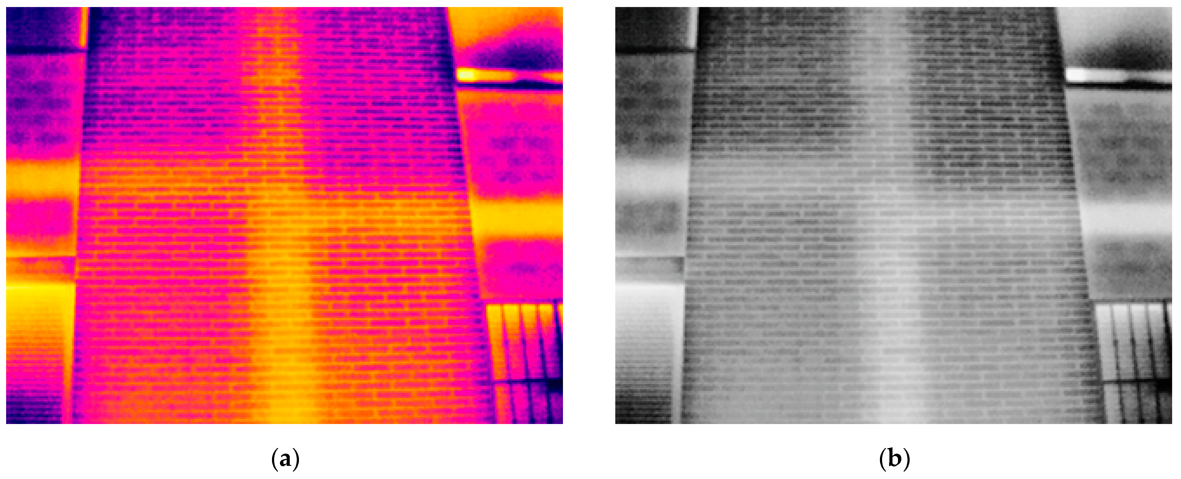
2.1. Thermal Imaging

The first stage of the proposed method is to record the façade building components’ temperature via IRT. In this research, this was carried out in two surveys in Andalusia, Spain (Figure 1): Survey A, in the south of the city of Seville (inland Mediterranean climate), and Survey B, in Alhaurin de la Torre, near Malaga (coastal Mediterranean climate).
The IRT surveys focused on the thermal bridge caused by the buildings’ reinforced concrete structure due to the lack of thermal insulation between the pillar and slabs and (1) the rendered brick façade (Survey A, a quasi-symmetrical sector), and (2) the vibrated concrete rough block façade (Survey B, a non-symmetrical sector).
The recording of the surface temperature in the IRT surveys is affected by changes in the directional emissivity due to different viewing angles (between the direction of the camera and the object’s emission direction) higher than 40° [30,31,32,33,34]. Moreover, the camera operators themselves constitute a source of emissions that must be taken into account by avoiding the perpendicularity between the camera direction and the object. These aspects were considered in the surveys of this research so that both procedural errors and environmental radiant sources, respectively, were minimised in the recording of the façades’ surface temperatures.
Besides, the weather conditions were recorded 24 h before the surveys using a portable weather station with sensors inside and outside the buildings. The hygrothermal indicators, input in both the camera settings and the thermographic software along with the material’s emissivity to produce the thermograms (graphical output of the IRT surveys), are gathered in Table 1.
Surveys A and B took place in winter and summer, respectively, and early in the morning to avoid direct sunlight as a radiation source; there was no rain or wind during the surveys. Additional considerations to minimise possible temperature reading errors and, therefore, errors when producing the 3D data, were avoiding targets with a temperature outside the thermal camera’s calibration range, such as the sky or extremely reflective surfaces [35]. The thermographic camera used was a FLIR E60bx, with an 18 mm FOL lens and resolution of 320 × 240 pixels. The camera was placed 6 m away from the façades in both surveys.
Once the data were recorded, this research used free thermographic software to produce the thermograms in the two cases. Flir Tools version 6.4.18039.1003 [36] allowed to input the infrared images, the hygrothermal indicators (Table 1), and the material’s emissivity coefficient [37] in the façades (0.85 and 0.92, respectively). In order to encompass all the possible temperature values in the thermograms, the range was set from 6.0 °C to 15 °C for Survey A, and from 22.0 °C to 27 °C for Survey B, given the ambient and surface temperatures in the scenes. The iron palette (colour configuration for thermograms) was firstly selected to show heat distribution and subtle details [38]. Still, the monochrome (grey) palette was chosen to ease image management in the GIS (Figure 2 and Figure 3).
It is worth noting that the temperature ranges specified above were not included in Figure 2 and Figure 3 as colour scales because these thermograms were exported for further processing. Finally, for the purpose of this research, it was necessary to extract the maximum and minimum temperature values from the thermograms (hottest and coldest points, respectively). Thus, the extent of the third dimension (of the 3D thermal data) could be next obtained from the temperature range using GIS.

2.2. GIS-Based Image Management

GIS are tools that facilitate the handling of geographic information rigorously in each process phase, such as data entry, storage, management, integration, edition, or visualisation. Their most common use is in work on the horizontal plane, as shown in the recent literature, such as [39,40,41,42,43]. By contrast, there are fewer cases for working with elevation [5,8], even if this only involves a change in coordinate axes.
In this work, a GIS has been used to carry out the thermogram’s geometric rectification and assign temperatures to the rectified image. QGIS v3.8.2 software [44] was used in this research.
In both surveys, it has been assumed that the area of interest is contained in a plane. Thus, the relief (depth) of the façade is not deemed. For this reason, instead of an orthorectification, only a 2D homography, or projective transformation is required. Here, eight parameters are considered to conduct perspective removal. This planar homography aims at transforming one plane into another, and can be expressed as [11]:
[ x y 1 ] = H [ X Y 1 ] = [ h 11   h 12   h 13   h 21   h 22   h 23   h 31   h 32   h 33   ] [ X Y 1 ]
Although the matrix presents nine parameters, the transformation poses eight degrees of freedom because the values are usually normalised, considering h33 = 1 (Figure 4). The eight parameters can be easily calculated from four pairs of points, both identified in the two spaces.
First, the geometrical measurement framework has to be defined. In this case, since this research presents a low-cost method, it has been preferred not to use classic topographical methods but a plumb, a spirit level, and a measuring tape.
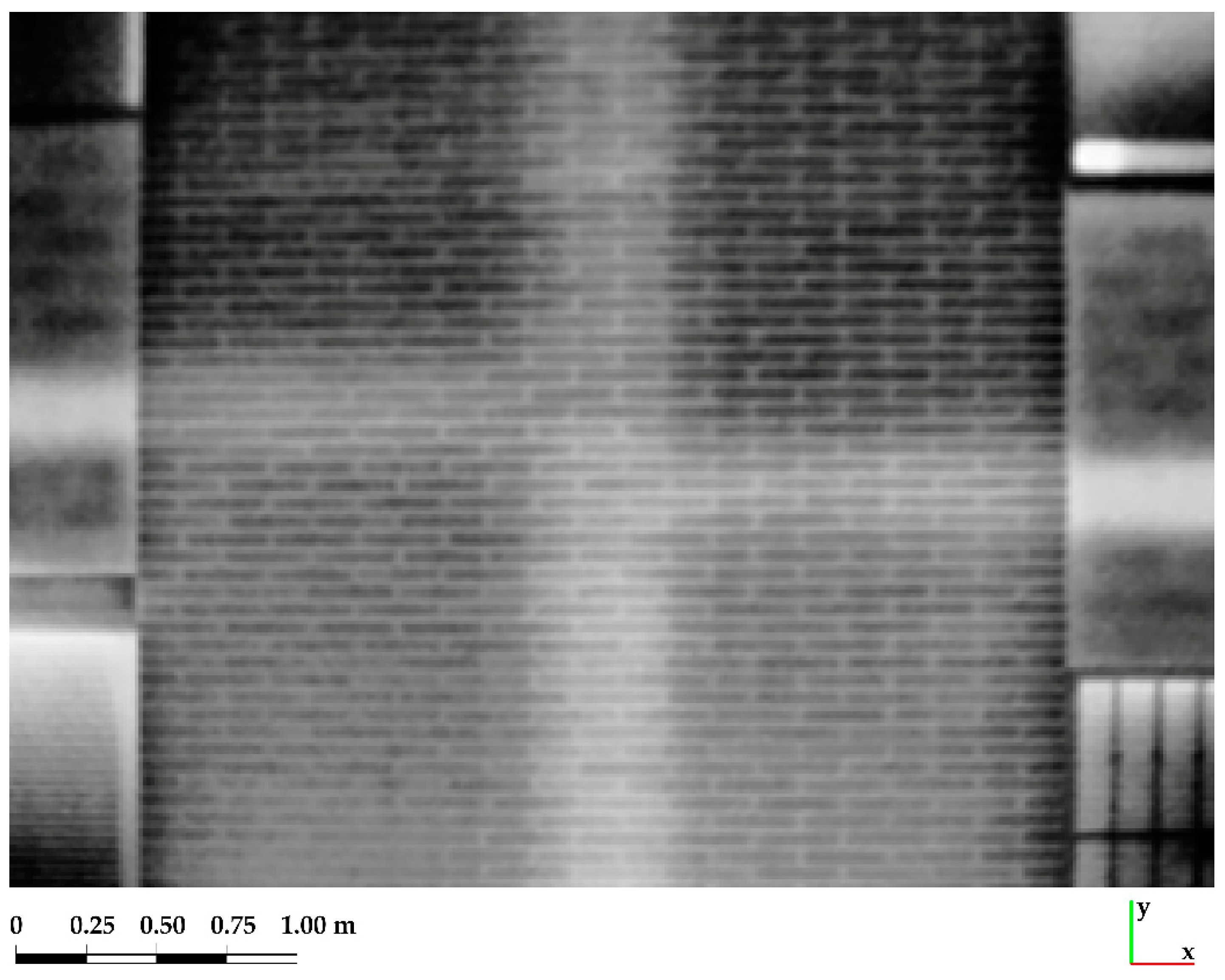
  • For Survey A, the façade itself served as a reference:
    -
    Y-axis: the (left) vertical limit of the façade;
    -
    X-axis: a mortar joint; a spirit level was used to check its horizontality.
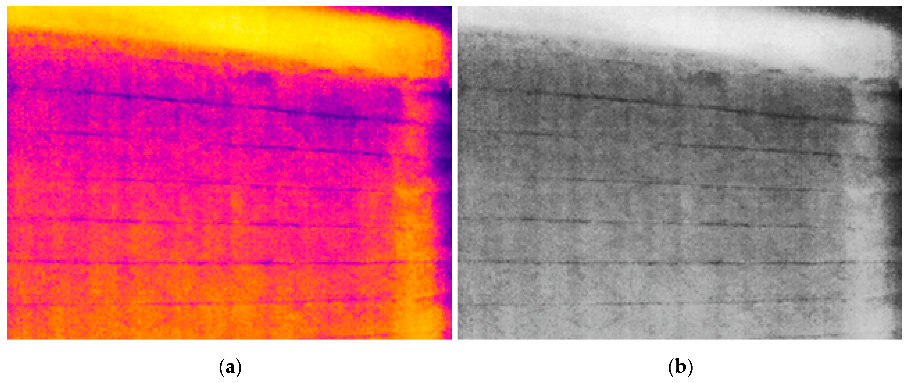
  • For Survey B:
    -
    Y-axis: a vertical joint, after checking with a plumb that its extension coincides with another of the lower joints;
    -
    X-axis: a horizontal mortar joint, whose horizontality has been verified using a spirit level.
Contrary to conventional topography, the distance measurements have been established a posteriori. To this end, it has been checked that the four points that will define the geometric frame are identifiable in the thermogram, using the diagonal as a verification. The measurements (and the axes) taken are displayed in Figure 5 on each thermogram.
Along with the geometrical 2D-homography, a radiometric conversion must be undertaken. Thereby, a digital number (DN) value must be assigned to each pixel of the resulting image. Besides, a bicubic interpolation has been chosen to conduct the resampling process.
After obtaining an image with the rectified geometry and the corresponding DN, the next step is for each pixel’s DN to correspond to the thermogram’s temperature. In both surveys, each thermogram was encoded on 8 bits, i.e., 256 values, as radiometric resolution. For the DN value to correlate with the temperature, a linear normalisation formula must be applied:
D N t e m p = a × D N + b
where a is the slope, that is related to the rectified image’s thermal sensitivity, and b is the intercept, the minimum temperature value. From the temperature values of each case, the calculated parameters are shown in Table 2. Thus, it can be concluded that the thermal resolution for the rectified image for Survey B is approximately three times better than that for Survey A:
For each pixel in the new image, the DN coincides with the temperature recorded. The image border has a dark background, which corresponds to the absence of data. This fact is inherent in any “photograph”. Due to the inclination, there will be points on the resampled image that lack information. The tilt is determined by the commitment to obtain an image covering as much spatial coverage as possible without a significant loss of geometric resolution (pixel size on the facade). This matter is especially relevant since the thermographic camera used only has 320 × 240 pixels.
Theoretically, a rectangular region of interest (hereinafter, ROI), in which all the pixels would have their temperature recorded, is more appropriate in terms of graphic language. However, this is not always suited, as information not included in the rectangle can be lost. This happens in survey B, where the slab thermal bridge above the rectangle has further temperature data.
Operating in a GIS environment allows fitting as much work area as possible by defining an area of interest that is not rectangular. This area has been used as a mask when exporting the data for the following processes.

2.3. 3D Point Cloud Data Treatment

For the purpose of this work, the three-dimensional data produced in the GIS platform need certain transformations to constitute the final 3D thermal data. This was carried out in CloudCompare v2.91 for 64-bit Microsoft Windows [45], although there are other open-source applications such as MeshLab [46] that can be used.
Firstly, the data were imported into the programme as the XYZ file created in the previous stage in GIS.
Next, a height ramp [47] or a height map of the 3D point set was generated to enhance the visualisation and readability of the 3D thermal data produced. This was performed using a monochrome linear gradient, 8-bit encoding (black for the lowest temperature, white for the highest), and a direction (Z-axis). The red, green and blue values of the RGB colours applied were therefore automatically associated with the coordinates of each point in the 3D point cloud.
It should be also noted that the temperature range of the thermograms determines the distribution of the points in the 3D thermal data. In other words, given that the third coordinate (Z) is represented in the three-dimensional thermal data as its temperature values (°C), it may be that these values are actually higher than the XY coordinates (dimensions of the object studied). As a result, interpretating the 3D point cloud’s proportions may not be easy. Therefore, to reduce the ”temperature-value/X-Y-dimensions” ratio, a scale factor of 0.10 was applied to the Z-axis (temperatures). Thus, a more representative 3D point set of the thermal behaviour of the façade was obtained.
Further management of the 3D thermal data makes it possible to gather useful information such as those façade sectors at a similar temperature. This can be carried out by creating point cloud contours by elevation (Z coordinate) thresholds. Considering that the Z-axis represents the temperature, these contours or 2D isolines—points with the same height or Z coordinate as in topographic maps—represent the thermogram isotherms—image regions within the same temperature range. The ”Rasterize” plugin [48] in CloudCompare helps create these isotherms by setting the gap (step) between the lines in the ”Contour plot” sub-tool, according to the temperature range of the façades. In this case, Survey B was considered to show the isotherms creation, conducted every 0.25°C from 23.25°C to 25.00°C. The contours can be exported in different file formats such as the broadly-used DXF. The results of the isotherm creation process are presented in the following section.
Finally, the ‘Rasterize’ plugin enables the creation of meshes from point clouds through the Delaunay 2.5D triangulation algorithm in the XY plane [49]. This is a suitable method to create 3D meshes from rather flat point clouds oriented to the Z-axis as in this research.

3. Results

In line with the methodology, this section is divided into the different technologies and processes considered in this research, particularly GIS and 3D point cloud data. The reason for not including the IRT results is that the thermograms from Surveys A and B are the method’s data source. Besides, they are already presented in Section 2.1 as an inherent part of the IRT surveys.

3.1. Image Management in GIS

The perspective correction was performed as per Section 2.3 to produce a rectangular ROI for the thermogram in Survey A. Nevertheless, given the slab’s thermal bridge in Survey B, the ROI selected included the thermal data of that area in the 3D point cloud (Figure 6).
In order to avoid duplication of figures, the rectified thermogram from Survey A will be presented in the following section as 3D thermal data.

3.2. 3D Thermal Data

Following Section 2.3, an 8-bit monochrome linear gradient height ramp was applied to the point sets, and a factor of 0.10 was next used to scale the Z-axis (temperature) to obtain a more representative 3D thermal data set (better point distribution) (Figure 7 and Figure 8).
Also, the top-view visualisation of the 3D height ramp produced shows the (rectified) original thermogram obtained using GIS as per Section 2.2. In turn, this helps to identify in 2D the most significant façade components or parts with the highest temperature and, consequently, those with the greatest energy loss (Figure 9 and Figure 10).
It should be noted that, when visualised in top view, the 3D thermogram from Survey B is not oblong as the one from Survey A because of the perspective correction into a rectangular shape. This is because the thermogram rectified in the GIS for Survey B includes the cropped area which was discarded after the image rectification as in Survey A. As a result, more radiometric data can be obtained by following the approach for Survey B.

3.2.1. Quantitative Analysis

Concerning the quantitative results that can be obtained from enquiring the 3D thermal data, diverse information about the thermal behaviour of the case studies can be obtained:
  • The proposed method produced 68,461 points from Survey A, whereas the 3D thermogram from Survey B contains 73,085 points (non-rectangular ROI), and 65,572 points (rectangular ROI);
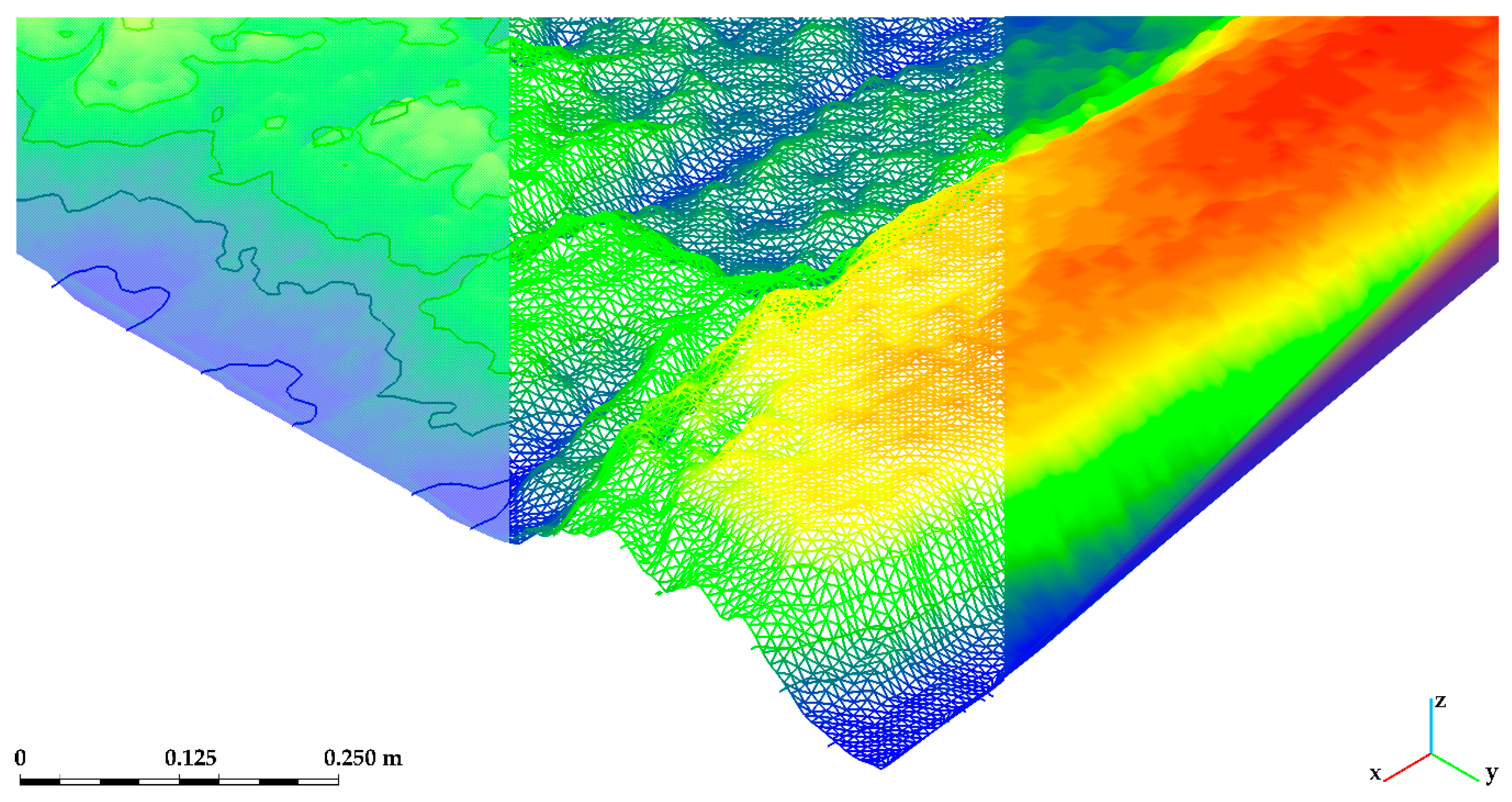
  • In Survey A, the temperature values (Z coordinate) enable to gather relevant information of the façade’s thermal behaviour. The lowest temperature is 7.011 °C, and the highest is 13.722 °C (6.710 °C temperature range). The average temperature of the façade is 9.895 °C, and the standard deviation is 1.165 °C.
  • In Survey B, the focus is on the non-rectangular thermogram, given the larger amount of thermal data produced against the rectangular ROI approach. The lowest temperature is 23.169 °C, and the highest is 25.164 °C (1.995 °C temperature range). The average temperature is 24.021 °C, and the standard deviation is 0.410 °C.
The distribution of temperatures is shown in the histograms for each survey in Figure 11 and Figure 12:
In view of Figure 11 and Figure 12, the most frequent temperature values are between 10.0 and 11.0 °C in Survey A, and between 23.5 and 24.5 °C in Survey B, approximately ―a difference of 1 °C in both cases.

3.2.2. From 3D Point Cloud Thermal Data to (2+1)D Isotherms and 3D Meshes

In order to provide additional quantitative and qualitative data from the 3D thermal point clouds, the ”Rasterize” plugin in CloudCompare [48] allows for creating isotherms and a 3D mesh from a point cloud. This was carried out for Survey B. The ‘Contour plot’ sub-tool was used to create planar isotherms, graded in the Z-axis (temperature) every 0.25 °C from 23.25 °C to 25.00 °C, given the temperature values in the case study (Figure 13).
Besides, the point cloud was discretised in order to create the 3D mesh displayed in the different modes in Figure 14.
The mesh produced contains 145,996 faces, approximately twice the number of vertices, as seen in Antón et al. [50]. In order to verify the accuracy of the meshing process [51], it is worth computing the distance between the scaled height-ramp cloud and the ”Rasterize”-tool mesh. This was conducted using the Multiscale Model to Model Cloud Comparison (M3C2) algorithm by Lague et al. [52] to measure the orthogonal distance between the mesh vertexes and the original 3D thermal data (the reference in the comparison). The reason for choosing the M3C2 method is that, according to its authors, it performs well in comparing point cloud data, even in complex 3D environments. Likewise, it is implemented in CloudCompare as a plugin [53], which eases the process given that there is no need to use different software to compute the point deviation. In this operation, the point normals (normal vectors of points) [54] of the original cloud (normals oriented to the Z-axis direction) were used to compute the distances. The mean distance was 0.00038 m, and the standard deviation was 0.000143 m; these data reveal the remarkable similarity between the point sets, given the negligible distance between homologous points. In fact, the comparison revealed that most of the points (70,825, which constitute 96.9% of the total of 73,085 points) are below 0.0001 m between the clouds.

4. Discussion and Conclusions

This final section is structured as follows: discussion of results from each stage in the methodology; research limitations; implications; and future work.

4.1. Discussion

About IRT, the results depicted in Figure 2 and Figure 3 (thermograms for further GIS processing) constitute the method’s data source. Consequently, this research does not aim at improving the IRT technology; the objective is to propose a new method to retrieve 3D thermal data from thermograms using GIS and 3D point cloud management software. Notwithstanding, it is worth discussing the IRT surveys and their outcomes. As described in Section 2.1, the surveys were chosen because of the existence of a thermal bridge caused by the reinforced concrete structure in both façades, which showed a quasi-symmetrical (Survey A) and a non-symmetrical (Survey B) configuration. Besides, apart from the considerations given to the survey conditions (time and season, and the lack of direct solar radiation, rain and wind), the importance of the hygrothermal conditions specified in Table 1 for an IRT survey should be discussed. According to Tran et al. [55], the ambient temperature determines the relative humidity; these two factors, including the interior temperature and relative humidity, have an impact on the heat flux, given that its natural trend is to reach equilibrium. Moreover, as seen in [35], water vapour in the atmosphere affects the infrared radiation recording. Finally, the use of IRT equipment and software has led to the generation of representative thermograms (IRT graphical output) of the thermal behaviour of each façade. They were exported as monochrome images (8 bits) for GIS processing to ease each pixel’s DN-temperature relation.
Regarding the GIS implementation, on the one hand, within the engineering graphics framework, perspective correction is an easy task using a GIS if the lens distortion is considered negligible compared to other parameters. In the case of a façade, checking the horizontality or verticality of certain features is very useful. Thus, although four points must be introduced into the 2D homography equations, three points can be enough data on some occasions as the forth could be deduced.
On the other hand, associating the temperature value to the Z coordinate enables 3D data plotting. Thereby, the X and Y coordinates would be the spatial variables of the data set-independent, since the geometry of the façade remains invariable. Conversely, the Z coordinate would be the thermal variable, which depends on the environmental conditions at the time of the survey and the construction characteristics of the façade element.
Concerning the management of the raw GIS point cloud, it should be highlighted that the 3D point cloud data processing software allows for treating these data to achieve a comprehensible data set. In this sense, given the extent of the Z coordinate in Surveys A and B’s thermal data in comparison to the XY coordinates, scaling the 3D data set in the Z-axis became necessary (see Figure 7 and Figure 8). Another process to enhance the data visualisation was creating a 3D heat map—Z-axis height ramp. As a result, the aforementioned spatial variables (X and Y coordinates) of the 3D thermal data can be seen in top view (orthogonal to Z-axis), which reveals the (rectified GIS) original thermogram as in Figure 9 and Figure 10. Thus, the 3D thermal data produced are representative of the thermal behaviour of the case studies as recorded by IRT.
Also, 2D isolines (isotherms) can be generated from the 3D thermal data produced by contour plotting in order to delimit the areas within the same established temperature range, which provides quantitative data of the façade sectors. In addition, as per Section 2.3, the point cloud can be discretised to create a 3D mesh with a high degree of accuracy. The combination of these isotherms and the mesh also enhance the dataset visualisation.
As to the histograms of the data from Surveys A and B, Figure 11 and Figure 12 reveal different point (temperature values in Z-axis) distributions. The reason for this is multiple: the temperature range of the 3D thermal data in Survey B (1.995 °C) is lower than that of Survey A (6.710 °C); and there is a higher number of hot areas in the latter, which are in turn less evenly distributed. This can be seen in the lower standard deviation values of Survey B 3D thermal data. It should be noted that the minimum and maximum temperature values in the 3D thermal data produced, and their temperature ranges, differ from those of the original IRT data. This is because the IRT software was used to manage the original (full) thermograms, whereas the GIS rectified thermograms were smaller since only the data within the ROI were considered in this research. Thus, the preliminary IRT extreme temperature values derive from the data out of the ROI; consequently, the 3D thermal data’s temperature values are correct.
Regarding the ROI, it should be noted that, because of the perspective correction in Survey B, the non-rectangular 3D thermal data set contains 73,085 points against the 65,572 points of the corresponding rectangular thermogram. Considering that there are 76,800 pixels in the original thermogram’s 320 × 240 pixel resolution, over 95% of the thermal information in the non-rectangular thermogram can be used for analysis, more than that of the rectangular ROI (over 85%). The 7513 points of difference between the two 3D thermograms from Survey B can be seen in both Figure 6a,b, and in Figure 8b (scaled point cloud). Those points belong to the slab thermal bridge in the façade. As can be seen in the isometric view and considering both their dimension in the Z-axis and the (gradient) colour code, the points present the greatest temperature values in Survey B’s 3D thermal data.
The symmetry of the 3D thermal data produced via the proposed method should also be discussed. As expected, Figure 7 and Figure 8, respectively, show quasi-symmetrical and non-symmetrical values in the Z coordinate (temperature) according to their original thermograms (Figure 2 and Figure 3, correspondingly).

4.2. Limitations

Concerning the limitations of the proposed method, it is first worth mentioning that IRT cannot record the temperature of hidden parts in the body (façade or object) except in some instances [13], as expected, nor those parts whose plane is in line with the direction of the camera. Thus, in the case of a façade as in Survey A (Figure 1), projections or overhangs cannot be measured from that point of view because of being perpendicular to the façade plane recorded via IRT. Hence, no 3D data will be obtained from those parts for that 3D thermogram. This issue can be addressed separately for each face as in the case of two perpendicular walls of a building with distinct temperature values among components. However, once combining the 3D thermal data of each face—in order to create a unique 3D thermogram—there may be an overlap of data between the walls if the temperature range (Z coordinate) is high. Nonetheless, this is not a problem in cases such as Survey B, where the temperature range is low; thus, the 3D point set’s dispersion is low, which prevents the operator from the data overlapping.
In relation to the image geometry, selecting a rectangular ROI is advisable in terms of graphical language. Given the angle of the IRT recording of the façade, the rectified thermogram contains regions with no data. This loss of thermal data could be minimised by increasing the distance between the IRT camera and the façade so that the thermal bridge is fully recorded. However, this entails larger pixel size in the thermograms, which means that the points used to conduct the rectification become less identifiable, and the thermal data ‘resolution’ decreases. This could be considered a limitation of the IRT equipment. In this research, the choice of a larger (non-rectangular) ROI in Survey B allows for minimising the loss of thermal information from the façade because of the recording perspective, as discussed above.

4.3. Implications

Regarding the average temperature of a sector, which can be obtained by enquiring the 3D thermal data produced in this research, it can be useful to calculate the thermal transmittance (U-value) of the building component studied [56]. The U-value calculation is useful to assess the thermal behaviour to ascertain whether or not it complies with the countries’ building regulations. This can be conducted as per Albatici and Tonelli’s Equation (3) [56,57]:
U = 5.67 ε tot   ( ( T m 100 4 ) ( T out 100 4 ) ) + 3.8054 v ( T m T out )   T int   T out ,
where U represents the thermal transmittance (W/m2K), Ɛtot is the integral emissivity (coefficient), Tm is the average temperature of the building component (K), Tint is the interior ambient temperature (K), Tout is the exterior ambient temperature (K), and v is the wind speed in m/s.
Therefore, considering that wind speed was 0.0 m/s in Surveys A and B in this research, the formula above turns into (Equation (4)):
U = 5.67 ε tot   ( ( T m 100 4 ) ( T out 100 4 ) )   T int   T out ,
This, in turn, becomes one of the applications that will next be described.
As seen in the introductory section, research into the specific topic of real-magnitude 3D thermal data visualisation of the thermal behaviour, as far as the present authors are concerned, has not been seen before. The 3D thermal data that can be produced using proprietary thermographic software differ from those of research into the creation of 3D thermographic or thermal models. The former, produced by software such as Avio InfReC Analyzer [14] or Fluke SmartView [15], are 3D representations (in 3D graphs) of the objects’ surface temperature. The latter consist of the mapping of thermographic textures onto 3D models or meshes of the objects’ surface. This research focuses on the former, the 3D representation of the objects’ temperature values, not on the mapping of the surface geometry of objects. Thereby, this work proposes a low-cost scientific research approach to produce real-magnitude 3D thermal data of buildings’ thermal behaviour for visualisation, analysis and interpretation. This research is based on the combination of different graphical technologies such as IRT, GIS and point cloud data processing software. In this sense, following the method proposed, radiometric data can be obtained by enquiring the 3D thermal point cloud data using any CAD or 3D environment software in the market. The findings of this research reveal that non-rectangular 3D thermograms from image rectification yield more 3D thermal data than considering traditional rectangular shapes. These data comprise temperature (single-point or average temperature of a sector), and the area of regions at the same temperature (between isotherms). Therefore, the significance of the proposed method resides in its capability to:
  • Produce both rectified 2D and 3D thermograms;
  • Retrieve radiometric information (temperature) from a non-radiometric raster image, even when the image is not rectangular;
  • Enable temperature and energy analyses from the spatial dataset;
  • Identify the most determining regions or elements in the body surveyed in terms of temperature and, therefore, energy loss;
Despite the limitations described above, and in view of the method’s capabilities mentioned in this subsection, this research has a broad range of applications due to IRT’s versatility. Among others, these are the energy audit of buildings and constructions; the thermal study of architectural, archaeological and cultural heritage for restoration; the identification and measuring of hot areas in computer hardware components, building services, or product quality control in the industry. Therefore, the method proposed in this paper is initially more suitable to be applied to (approximately) flat surfaces. This is because a GIS is used in this research to restore the objects’ real dimensions. Thereby, the image distortion is corrected to obtain an orthogonal view that guarantees that the temperature is represented by the Z-axis in an adequate coordinate system. In contrast, in curved and other non-flat objects, the recording of the surface temperature in the IRT survey is affected by the aforementioned directional emissivity [30,31,32,33,34]. This entails that the temperature (Z coordinate), initially, could not be a reliable value of the 3D thermal data of the object. However, according to Campione et al. [58], this can be corrected in concave and convex geometries, which increases the possible applications of the proposed method to non-flat objects.

4.4. Future Work

Future work on this research involves working on the bodies’ out-of-plane parts and perpendicular faces to combine their 3D thermal data with the main bodies’ data without overlapping. Moreover, an ad hoc script can be developed to automate the analysis of the 3D thermal data produced: the creation of isotherms; the calculation of their area; the calculation of the minimum, maximum and average temperatures; and the corresponding thermal transmittance value. Regarding the future GIS-related work, another possible investigation is related to the design and placement of thermal targets on the façades for IRT recording. Along with the implementation of an algorithm in QGIS, this would automate the image rectification, the homography between the original thermogram and the plane of the façade. In view of the results in this research, the image rectification would be performed by considering non-rectangular thermograms to increase the amount of 3D thermal data.

Author Contributions

Conceptualization, D.A. and J.-L.A.-M.; methodology, D.A. and J.-L.A.-M.; software, D.A. and J.-L.A.-M.; validation, D.A. and J.-L.A.-M.; formal analysis, D.A. and J.-L.A.-M.; investigation, D.A. and J.-L.A.-M.; resources, D.A. and J.-L.A.-M.; data curation, D.A. and J.-L.A.-M.; writing—original draft preparation, D.A. and J.-L.A.-M.; writing—review and editing, D.A. and J.-L.A.-M.; visualization, D.A. and J.-L.A.-M.; supervision, D.A. and J.-L.A.-M.; project administration, D.A. and J.-L.A.-M.; funding acquisition, D.A. All authors have read and agreed to the published version of the manuscript.

Funding

This research was funded by Universidad de Sevilla through VI Plan Propio de Investigación y Transferencia (VIPPIT), grant number CONV-822 and VIPPIT-2019-II.3.

Institutional Review Board Statement

Not applicable.

Informed Consent Statement

Not applicable.

Data Availability Statement

The data presented in this study is contained within the article.

Acknowledgments

The Authors wish to acknowledge the Departamento de Expresión Gráfica e Ingeniería en la Edificación of Universidad de Sevilla for access to the infrared camera and portable weather station.

Conflicts of Interest

The authors declare no conflict of interest. The funders had no role in the design of the study; in the collection, analyses, or interpretation of data; in the writing of the manuscript, or in the decision to publish the results.

References

  1. Sorby, S. Developing 3D spatial visualization skills. Eng. Des. Graph. J. 1999, 63, 21–32. [Google Scholar]
  2. Marunic, G.; Glazar, V. Spatial ability through engineering graphics education. Int. J. Technol. Des. Educ. 2013, 23, 703–715. [Google Scholar] [CrossRef]
  3. Ruiz-Jaramillo, J.; Mascort-Albea, E.; Jaramillo-Morilla, A. Proposed methodology for measurement, survey and assessment of vertical deformation of structures. Struct. Surv. 2016, 34, 276–296. [Google Scholar] [CrossRef]
  4. Volk, R.; Stengel, J.; Schultmann, F. Building Information Modeling (BIM) for existing buildings—Literature review and future needs. Autom. Constr. 2014, 38, 109–127. [Google Scholar] [CrossRef] [Green Version]
  5. Lerma, J.L.; Navarro, S.; Cabrelles, M.; Portalés, C. Implementation of an Architectonic GIS on a Brickwork Farmhouse. In International Archives of the Photogrammetry, Remote Sensing and Spatial Information Sciences—ISPRS Archives; Chen, J., Jiang, J., Maas, H.-G., Eds.; International Society for Photogrammetry and Remote Sensing, Inc. (ISPRS): Beijing, China, 2008; pp. 1013–1015. [Google Scholar]
  6. Previtali, M.; Erba, S.; Rosina, E.; Redaelli, V.; Scaioni, M.; Barazzetti, L. Generation of a GIS-based environment for infrared thermography analysis of buildings. In Infrared Remote Sensing and Instrumentation XX; Strojnik, M., Paez, G., Eds.; Society of Photographic Instrumentation Engineers: Bellingham, WA, USA, 2012; p. 85110U. [Google Scholar]
  7. Yuanrong, H.; Jiaquan, D.; Shenghui, C.; Degui, P. Facade measurement of building along the roadway based on TLS and GIS of project supervision. In IOP Conference Series: Earth and Environmental Science; IOP Publishing: Bristol, UK, 2018; Volume 146, p. 012027. [Google Scholar]
  8. Chen, K.; Reichard, G.; Xu, X. GIS-Based Modeling of Multi-Sourced Image Data Collected for Building Facade Inspection. In Construction Research Congress 2020; American Society of Civil Engineers: Reston, VA, USA, 2020; pp. 866–875. [Google Scholar]
  9. Wang, Y.; Fan, H.; Zhou, G. Reconstructing facade semantic models using hierarchical topological graphs. Trans. GIS 2020, 24, 1073–1097. [Google Scholar] [CrossRef]
  10. Yue, L.; Li, H.; Zheng, X. Distorted Building Image Matching with Automatic Viewpoint Rectification and Fusion. Sensors 2019, 19, 5205. [Google Scholar] [CrossRef] [Green Version]
  11. Soycan, A.; Soycan, M. Perspective correction of building facade images for architectural applications. Eng. Sci. Technol. Int. J. 2019, 22, 697–705. [Google Scholar] [CrossRef]
  12. Balaras, C.A.; Argiriou, A.A. Infrared thermography for building diagnostics. Energy Build. 2002, 34, 171–183. [Google Scholar] [CrossRef]
  13. Glavaš, H.; Hadzima-Nyarko, M.; Haničar Buljan, I.; Barić, T. Locating Hidden Elements in Walls of Cultural Heritage Buildings by Using Infrared Thermography. Buildings 2019, 9, 32. [Google Scholar] [CrossRef] [Green Version]
  14. Nippon Avionics Company InfReC Analyzer NS9500 Professional; Nippon Avionics Co., Ltd.: Tokyo, Japan, 2020.
  15. Fluke SmartView IR Analysis Reporting Software; Fluke Corporation: Everett, WA, USA, 2013.
  16. Paramasivam, B. Investigation on the effects of damping over the temperature distribution on internal turning bar using Infrared fusion thermal imager analysis via SmartView software. Meas. J. Int. Meas. Confed. 2020, 162, 107938. [Google Scholar] [CrossRef]
  17. Shchegolkov, A.; Shchegolkov, A.; Demidova, A. The use of nanomodified heat storage materials for thermal stabilization in the engineering and aerospace industry as a solution for economy. In International Conference on Modern Trends in Manufacturing Technologies and Equipment 2018 (ICMTMTE 2018); Bratan, S., Gorbatyuk, S., Leonov, S., Roshchupkin, S., Eds.; EDP Sciences: Sevastopol, Russia, 2018; Volume 224, p. 03012. [Google Scholar]
  18. Alba, M.I.; Barazzetti, L.; Scaioni, M.; Rosina, E.; Previtali, M. Mapping Infrared Data on Terrestrial Laser Scanning 3D Models of Buildings. Remote Sens. 2011, 3, 1847–1870. [Google Scholar] [CrossRef] [Green Version]
  19. Vidas, S.; Moghadam, P.; Bosse, M. 3D thermal mapping of building interiors using an RGB-D and thermal camera. In 2013 IEEE International Conference on Robotics and Automation; IEEE: Piscataway, NJ, USA, 2013; pp. 2311–2318. [Google Scholar]
  20. Wang, C.; Cho, Y.K.; Gai, M. As-Is 3D Thermal Modeling for Existing Building Envelopes Using a Hybrid LIDAR System. J. Comput. Civ. Eng. 2013, 27, 645–656. [Google Scholar] [CrossRef]
  21. Borrmann, D.; Elseberg, J.; Nüchter, A. Thermal 3D mapping of building façades. In Advances in Intelligent Systems and Computing; Springer: Berlin/Heidelberg, Germany, 2013; Volume 193 AISC, pp. 173–182. [Google Scholar]
  22. Rangel, J.; Soldan, S.; Kroll, A. 3D Thermal Imaging: Fusion of Thermography and Depth Cameras. In Proceedings of the 12th International Conference on Quantitative Infrared Thermography (QIRT 2014), Bordeaux, France, 7–11 July 2014. [Google Scholar]
  23. Ham, Y.; Golparvar-Fard, M. 3D Visualization of thermal resistance and condensation problems using infrared thermography for building energy diagnostics. Vis. Eng. 2014, 2, 1–15. [Google Scholar] [CrossRef] [Green Version]
  24. Moghadam, P.; Vidas, S. HeatWave: The next generation of thermography devices. In Thermosense: Thermal Infrared Applications XXXVI; Colbert, F.P., Hsieh, S.-J., Eds.; Society of Photographic Instrumentation Engineers: Bellingham, WA, USA, 2014; p. 91050F. [Google Scholar]
  25. Moghadam, P. 3D medical thermography device. In Thermosense: Thermal Infrared Applications XXXVII; Hsieh, S.-J., Zalameda, J.N., Eds.; International Society for Optics and Photonics (SPIE): Bellingham, WA, USA, 2015; Volume 9485, p. 94851J. [Google Scholar]
  26. Matsumoto, K.; Nakagawa, W.; Saito, H.; Sugimoto, M.; Shibata, T.; Yachida, S. AR Visualization of Thermal 3D Model by Hand-held Cameras. In Proceedings of the 10th International Conference on Computer Vision Theory and Applications; SCITEPRESS—Science and Technology Publications: Setúbal, Portugal, 2015; Volume 3, pp. 480–487. [Google Scholar]
  27. Nakagawa, W.; Matsumoto, K.; de Sorbier, F.; Sugimoto, M.; Saito, H.; Senda, S.; Shibata, T.; Iketani, A. Visualization of Temperature Change Using RGB-D Camera and Thermal Camera. In Lecture Notes in Computer Science; Including Subseries Lecture Notes in Artificial Intelligence and Lecture Notes in Bioinformatics; Springer: Berlin/Heidelberg, Germany, 2015; Volume 8925, pp. 386–400. ISBN 9783319161778. [Google Scholar]
  28. Natephra, W.; Motamedi, A.; Yabuki, N.; Fukuda, T.; Michikawa, T. Building Envelope Thermal Performance Analysis using BIM-Based 4D Thermal Information Visualization. In Proceedings of the 16th International Conference on Computing in Civil and Building Engineering (ICCCBE2016); Yabuki, N., Makanae, K., Eds.; ICCCBE2016 Organizing Committee: Osaka, Japan, 2016; pp. 1539–1546. [Google Scholar]
  29. Landmann, M.; Heist, S.; Dietrich, P.; Lutzke, P.; Gebhart, I.; Templin, J.; Kühmstedt, P.; Tünnermann, A.; Notni, G. High-speed 3D thermography. Opt. Lasers Eng. 2019, 121, 448–455. [Google Scholar] [CrossRef]
  30. Ianiro, A.; Cardone, G. Measurement of surface temperature and emissivity with stereo dual-wavelength IR thermography. J. Mod. Opt. 2010, 57, 1708–1715. [Google Scholar] [CrossRef]
  31. Cheng, T.Y.; Deng, D.; Herman, C. Curvature effect quantification for in-vivo IR thermography. In ASME International Mechanical Engineering Congress and Exposition, Proceedings (IMECE); NIH Public Access: Bethesda, MD, USA, 2012; Volume 2, pp. 127–133. [Google Scholar]
  32. Gutierrez, E.; Castañeda, B.; Treuillet, S. Correction of Temperature Estimated from a Low-Cost Handheld Infrared Camera for Clinical Monitoring. In Lecture Notes in Computer Science; Including Subseries Lecture Notes in Artificial Intelligence and Lecture Notes in Bioinformatics; Springer: Berlin/Heidelberg, Germany, 2020; Volume 12002 LNCS, pp. 108–116. ISBN 9783030406042. [Google Scholar]
  33. Cardone, G.; Ianiro, A.; Dello Ioio, G.; Passaro, A. Temperature maps measurements on 3D surfaces with infrared thermography. Exp. Fluids 2012, 52, 375–385. [Google Scholar] [CrossRef]
  34. Greco, C.S.; Paolillo, G.; Contino, M.; Caramiello, C.; Di Foggia, M.; Cardone, G. 3D temperature mapping of a ceramic shell mould in investment casting process via infrared thermography. Quant. Infrared Thermogr. J. 2020, 17, 40–62. [Google Scholar] [CrossRef]
  35. Fluke Corporation. Fluke SmartView Manual. Available online: https://dam-assets.fluke.com/s3fs-public/SmartV__pheng0100.pdf (accessed on 14 December 2020).
  36. FLIR. Systems Flir Tools; FLIR: Wilsonville, OR, USA, 2018. [Google Scholar]
  37. ThermoWorks. Infrared Emissivity Table. Available online: https://www.thermoworks.com/emissivity-table (accessed on 12 December 2020).
  38. FLIR Systems. Your Perfect Palette. Available online: https://www.flir.co.uk/discover/ots/outdoor/your-perfect-palette/ (accessed on 14 December 2020).
  39. Al-Kindi, K.M.; Alkharusi, A.; Alshukaili, D.; Al Nasiri, N.; Al-Awadhi, T.; Charabi, Y.; El Kenawy, A.M. Spatiotemporal Assessment of COVID-19 Spread over Oman Using GIS Techniques. Earth Syst. Environ. 2020, 4, 797–811. [Google Scholar] [CrossRef]
  40. Ali, S.A.; Khatun, R.; Ahmad, A.; Ahmad, S.N. Assessment of Cyclone Vulnerability, Hazard Evaluation and Mitigation Capacity for Analyzing Cyclone Risk using GIS Technique: A Study on Sundarban Biosphere Reserve, India. Earth Syst. Environ. 2020, 4, 71–92. [Google Scholar] [CrossRef]
  41. Al Baky, M.A.; Islam, M.; Paul, S. Flood Hazard, Vulnerability and Risk Assessment for Different Land Use Classes Using a Flow Model. Earth Syst. Environ. 2020, 4, 225–244. [Google Scholar] [CrossRef] [Green Version]
  42. Navarro Cerrillo, R.M.; Palacios Rodríguez, G.; Clavero Rumbao, I.; Lara, M.Á.; Bonet, F.J.; Mesas-Carrascosa, F.-J. Modeling Major Rural Land-Use Changes Using the GIS-Based Cellular Automata Metronamica Model: The Case of Andalusia (Southern Spain). ISPRS Int. J. Geo-Inf. 2020, 9, 458. [Google Scholar] [CrossRef]
  43. Kulawiak, M.; Dawidowicz, A.; Pacholczyk, M.E. Analysis of server-side and client-side Web-GIS data processing methods on the example of JTS and JSTS using open data from OSM and geoportal. Comput. Geosci. 2019, 129, 26–37. [Google Scholar] [CrossRef]
  44. QGIS Development Team. QGIS Geographic Information System. 2020. Available online: https://qgis.org/en/site/getinvolved/faq/index.html#how-to-cite-qgis (accessed on 18 February 2021).
  45. Girardeau-Montaut, D. 3D Point Cloud and Mesh Processing Software; CloudCompare: Amsterdam, The Netherlands, 2016. [Google Scholar]
  46. Cignoni, P.; Callieri, M.; Corsini, M.; Dellepiane, M.; Ganovelli, F.; Ranzuglia, G. MeshLab: An Open-Source Mesh Processing Tool. In Proceedings of the Sixth Eurographics Italian Chapter Conference; Scarano, V., Chiara, R.D., Erra, U., Eds.; The Eurographics Association: Salerno, Italy, 2008; pp. 129–136. [Google Scholar]
  47. Girardeau-Montaut, D. Colors\Height Ramp. Available online: https://www.cloudcompare.org/doc/wiki/index.php?title=Colors%5CHeight_Ramp (accessed on 21 December 2020).
  48. Girardeau-Montaut, D. Rasterize. Available online: https://www.cloudcompare.org/doc/wiki/index.php?title=Rasterize (accessed on 29 December 2020).
  49. Girardeau-Montaut, D. Mesh\Delaunay 2.5D (XY Plane). Available online: https://www.cloudcompare.org/doc/wiki/index.php?title=Mesh%5CDelaunay_2.5D_(XY_plane) (accessed on 29 December 2020).
  50. Antón, D.; Medjdoub, B.; Shrahily, R.; Moyano, J. Accuracy evaluation of the semi-automatic 3D modeling for historical building information models. Int. J. Archit. Herit. 2018, 12, 790–805. [Google Scholar] [CrossRef] [Green Version]
  51. Antón, D.; Pineda, P.; Medjdoub, B.; Iranzo, A. As-Built 3D Heritage City Modelling to Support Numerical Structural Analysis: Application to the Assessment of an Archaeological Remain. Remote Sens. 2019, 11, 1276. [Google Scholar] [CrossRef] [Green Version]
  52. Lague, D.; Brodu, N.; Leroux, J. Accurate 3D comparison of complex topography with terrestrial laser scanner: Application to the Rangitikei canyon (N-Z). ISPRS J. Photogramm. Remote Sens. 2013, 82, 10–26. [Google Scholar] [CrossRef] [Green Version]
  53. Girardeau-Montaut, D. M3C2 (Plugin). Available online: https://www.cloudcompare.org/doc/wiki/index.php?title=M3C2_(plugin) (accessed on 29 December 2020).
  54. Girardeau-Montaut, D. Normals\Compute. Available online: https://www.cloudcompare.org/doc/wiki/index.php?title=Normals%5CCompute (accessed on 28 November 2018).
  55. Tran, Q.H.; Han, D.; Kang, C.; Haldar, A.; Huh, J. Effects of Ambient Temperature and Relative Humidity on Subsurface Defect Detection in Concrete Structures by Active Thermal Imaging. Sensors 2017, 17, 1718. [Google Scholar] [CrossRef]
  56. Moyano Campos, J.J.; Antón García, D.; Rico Delgado, F.; Marín García, D. Threshold Values for Energy Loss in Building Façades Using Infrared Thermography. In Sustainable Development and Renovation in Architecture, Urbanism and Engineering; Mercader-Moyano, P., Ed.; Springer: Cham, Switzerland, 2017; pp. 427–437. ISBN 978-3-319-51442-0. [Google Scholar]
  57. Albatici, R.; Tonelli, A.M. Infrared thermovision technique for the assessment of thermal transmittance value of opaque building elements on site. Energy Build. 2010, 42, 2177–2183. [Google Scholar] [CrossRef]
  58. Campione, I.; Lucchi, F.; Santopuoli, N.; Seccia, L. 3D Thermal Imaging System with Decoupled Acquisition for Industrial and Cultural Heritage Applications. Appl. Sci. 2020, 10, 828. [Google Scholar] [CrossRef] [Green Version]
Figure 1. Location of IRT Surveys A and B.
Symmetry 13 00335 g001
Figure 2. Thermograms of Survey A for GIS processing: (a) Iron palette; (b) Grey (monochrome) palette.
Symmetry 13 00335 g002
Figure 3. Thermograms of Survey B for GIS processing: (a) Iron palette; (b) Grey (monochrome) palette.
Symmetry 13 00335 g003
Figure 4. Homographic transformation to remove the perspective distortion.
Symmetry 13 00335 g004
Figure 5. Measurements taken for perspective correction: (a) Survey A; (b) Survey B.
Symmetry 13 00335 g005
Figure 6. Rectified thermograms from Survey B: (a) Rectangular image; (b) Better-fitted image.
Symmetry 13 00335 g006
Figure 7. Isometric view of the 3D thermal data from Survey A: (a) original height-map 3D thermal data; (b) scaled height-map 3D thermal data.
Symmetry 13 00335 g007
Figure 8. Isometric view of the 3D thermal data from Survey B: (a) original height-map 3D thermal data; (b) scaled height-map 3D thermal data.
Symmetry 13 00335 g008
Figure 9. Top view of the 3D thermal data from Survey A.
Symmetry 13 00335 g009
Figure 10. Top view of the 3D thermal data from Survey B.
Symmetry 13 00335 g010
Figure 11. 3D thermal data distribution in Survey A.
Symmetry 13 00335 g011
Figure 12. 3D thermal data distribution in Survey B.
Symmetry 13 00335 g012
Figure 13. Top view of the isotherms from the 3D thermal data in Survey B.
Symmetry 13 00335 g013
Figure 14. Isometric view of the 3D thermal data from Survey B: (left) Isotherms; (centre) Wireframe mesh and isotherms; (right) Solid mesh.
Symmetry 13 00335 g014
Table 1. Hygrothermal conditions in surveys A and B.
SchemeDate and TimeExterior Temperature (°C)Interior Temperature (°C)Atmospheric Pressure (mbar)Exterior HR (%)Interior HR (%)
A28/01/2016 6:11 a.m.9.018.710539172
B02/09/2016 8:22 a.m.22.628.610208767
HR represents the relative humidity. Wind speed was 0 m/s.
Table 2. Extreme temperatures and conversion parameters for each survey.
SchemeTmin (°C)Tmax (°C)DNminDNmaxab
A6.914.002550.027846.9
B23.025.402550.0094123.0
Publisher’s Note: MDPI stays neutral with regard to jurisdictional claims in published maps and institutional affiliations.

