Sliding Mode Control and Geometrization Conjecture in Seismic Response

Abstract

The purpose of this paper is to study the sliding mode control as a Ricci flow process in the context of a three-story building structure subjected to seismic waves. The stability conditions result from two Lyapunov functions, the first associated with slipping in a finite period of time and the second with convergence of trajectories to the desired state. Simulation results show that the Ricci flow control leads to minimization of the displacements of the floors.

1. Introduction

In recent years, the algorithms applied to control building systems subjected to seismic loads have been studied extensively [1,2]. The sliding mode control arises as a variable control, which constrains the structure to lie within a neighborhood of the switching function [3]. A series of phenomena in mechanics and other fields exhibit discontinuities, with respect to the current state in the differential equations that describe their behavior. An example is the Coulomb dry friction process, whose resistance force depends on the motion direction. Additionally, for the automatic control, minimizing the power consumed for the control purposes or restricting the range of variation of the control parameters leads to interruptions [4]. The aim of the control is to tailor the structure behavior with respect to a choice of the switching function, in terms of insensitivity or any uncertainties [5]. Optimization and control of the sliding modes are discussed in [6].

The sliding mode is associated with a discontinuity surface $s$ whenever the distances to this surface and the velocity of its change are of opposite signs, i.e., when [6]

$${\lim }_{s\to -0} \dot{s}>0 \mathrm{and} {\lim }_{s\to +0} \dot{s}<0.$$

A discontinuous dynamic system may be described by the equation

$$\dot{x}=f(x,t),$$

(1)

where $x\in R^n$ is the state vector, $t$ is time, and $f(x,t)$ has discontinuities in the form of points, lines, or surfaces within the $(n+1)$-dimensional space $(x,t)$.

For example, for the equation

$$m\ddot{x}+P(\dot{x})+kx=0,$$

(2)

where $x$ is the displacement, $m$ the mass, and $k$ is the spring rigidity and

$$P(\dot{x})=\{\begin{array}{r}{P}_0,\hspace{0.17em}\hspace{0.17em}\hspace{0.17em}\hspace{0.17em}\hspace{0.17em}\mathrm{for} \dot{x}>0\\ -P_0,\hspace{0.17em}\hspace{0.17em}\hspace{0.17em}\hspace{0.17em}\hspace{0.17em}\mathrm{for} \dot{x}<0\end{array},$$

(3)

where $P_0>0$ is a constant and the discontinuity surface is the $x$-axis [6]

$$s=\dot{x}=0.$$

(4)

Various control algorithms and control devices have been investigated for adaptive sliding mode control [7]. New methodologies include the optimal control, the stochastic control, the adaptive control, the hybrid control, and the intelligent control [8].

The piecewise-continuous dynamic systems to filtering problems are discussed in [9,10]. In the following, we use the Ricci flow, the trajectories moving on a manifold to model the sliding mode control, and the structure response to seismic loadings. The condition of the system trajectories to stay and move on the Riemannian 2-manifold $(M^2,g)$, for which $s=0$, can be modeled as the Ricci flow defined on a manifold $(\overline{M},g)$ as [11,12]

$$\frac{\partial g}{\partial t}=-2\mathrm{Ricci}(g)$$

(5)

The Ricci soliton was introduced by Hamilton in order to proof the 3D sphere theorem [11]. In 2002 and 2003, Perelman stated a new version of the Hamilton’s method [12,13]. He was awarded a Fields medal in 2006 for his contributions but he declined to accept it. A survey on Ricci solitons on Riemannian submanifolds is found in [14].

The Ricci flow is often thought as a tensor written in local coordinates by simple formulae involving the first and second derivatives of the metric tensor [15,16,17,18,19,20,21]. Many results for Ricci flow are related to the mean curvature flow of hypersurfaces. The Ricci curvature is a measure of the degree to which the geometry of a given metric tensor differs locally from that of ordinary Euclidean space or pseudo-Euclidean space.

The fixed points of (5) are called Ricci solitons. In order to find the fixed points of (5) on the diffeomorphism of $\overline{M}$ and scaling of $g$, (5) is rewritten as [14]

$$-2\mathrm{Ricci}(g)=L_{X}g+2\mathsf{\lambda }g$$

(6)

where $L_{E}g$ is the Lie derivation of $g$, with respect to any vector $X$, and $\mathsf{\lambda }>0$ is a constant.

On the Riemannian manifold $(\overline{M},g)$, we have for any vector $X$ the condition [14]

$$(L_{X}g)\frac{\partial }{\partial t}(L_{X}g)\le -\mathsf{\eta }|L_{X}g|,$$

(7)

which ensures that the vector belongs to $\overline{M}$, where $\nabla$ is the Levi–Civita connection of the metric $g$. The system trajectories of the structure stay and move on the Riemannian 2-manifold $(M^2,g)$ for any point $P\in M^2$ if and only if the condition (7) is verified [15,16,17]. A solution of (6) is given by [14]

$$g(t)=c(t){\mathsf{\psi }}_t^{*}g,$$

(8)

where $c(t)$ is a function of $t$ and ${\mathsf{\psi }}_t$ is a family of diffeomorphisms with $c(0)=1$ $\mathsf{\psi }(0)=\mathrm{i}{d}_0$, $d_0=\min d(r)$, $\forall P\subset M^2$, and $\mathsf{\lambda }=\frac{c^{\prime }(0)}{2}$. If $X=\mathrm{grad}F$ for an arbitrary function, for $F$ we have [14]

$$L_{X}g=2\nabla \mathrm{d}F$$

(9)

Our approach was to reduce the state equation of a three-story building subjected to seismic loads to the Ricci soliton Equation (5). This does not imply that we no longer applied the modal analysis but does imply that the sliding control for vibration control was performed simply and efficiently.

2. Sliding Mode Control

To implement the condition (7) to structural design, we considered a three-story building structure subjected to seismic waves, shown in Figure 1. The structure was idealized as a three-lumped-mass shear-beam model subjected to shear force at the base $F(t)$.

In Figure 1, $m_i,i=1,2,3$ are the masses, $c_i,i=1,2,3$ are the structural damping coefficients, $k_i,i=1,2,3$ are the stiffness coefficients, and $x_i(t),i=1,2,3$ are the masses displacements. The motion equation for the three-story building is given by

$$M\hspace{0.17em}\frac{{\partial }^{2}x}{\partial t^2}+C\frac{\partial x}{\partial t}+Kx(t)=B_{1}u(t)+E_{1}F(t)$$

(10)

where $x(t)=[x_1,x_2,x_3]$ is the vector of displacements $x_i(t),i=1,2,3$ of the i- th story relative to the ground, $M$,$C$ and $K$ represent the mass, damping, and stiffness matrices, respectively, $B_1$ is the location matrix for the control forces, and $E_1$ is the location matrix of external loads $F(t)$. Equation (10) can be rewritten as

$$\frac{\partial z}{\partial t}=Az(t)+Bu(t)+EF(t), z(0)=z_0,$$

(11)

where $z(t)={\left[x(t),\frac{\partial x}{\partial t}\right]}^T$ is the state vector, $z_0$ is a initial trajectory we need for the control design, and the matrices $A,B$ and $E$ are

$$A=\left[\begin{array}{cc}0& I\\ -M^{-1}K& -M^{-1}C\end{array}\right], B=\left[\begin{array}{c}0\\ M^{-1}{B}_1\end{array}\right], E=\left[\begin{array}{c}0\\ M^{-1}{E}_1\end{array}\right]$$

(12)

We consider the doubly warped product metrics of the form

$$g={\mathrm{dz}}_1^2+Az{\mathrm{dz}}_2^2+Cf{\mathrm{dz}}_3^2, Cf=Bu+EF,$$

(13)

where ${\mathrm{dz}}_2^2$ and ${\mathrm{dz}}_3^2$ are considered as metrics on a sphere and an Einstein manifold, respectively [15]. Let $N^2=R^2$ with metric $h={\mathrm{dz}}_1^2+Az{\mathrm{dz}}_2^2$ and let $\mathsf{\phi }:(R^3,g)\to (R^2,h)$ be the projection $\mathsf{\phi }(z_1,z_2,z_3)=(z_1,z_2).$ Then $\mathsf{\phi }$ is semi-conformal with $\mathsf{\lambda }=1$ and with a corresponding form dual to its kernel $\mathsf{\theta }=\sqrt{Cf}{\mathrm{dz}}_3$.

The dual of the mean curvature is $\mathsf{\mu }=d\ln b^{-1}$, so that $\mathsf{\rho }=b^{-1}$ and

$$\mathrm{d}\mathsf{\theta }+\mathrm{d}\ln \mathsf{\rho }\mathsf{\theta }=0$$

(14)

Then, (13) becomes

$$g=\mathsf{\phi }h+{\mathsf{\theta }}^2$$

(15)

and the Ricci flow is written under the form

$$\frac{\partial z}{\partial t}=-2\mathrm{Ricci}(z)=Az(t)+Bu(t)+EF(t), z(0)=z_0$$

(16)

A possible choice of the sliding mode controller is proposed in [22]

$$u=-\mathsf{\eta }\mathrm{sgn}(s)+u_{eq}$$

(17)

where $\mathrm{sgn}$ is the sign function and $u_{eq}$ is the equivalent control for the system states in the sliding mode. The constant $\mathsf{\eta }>0$ represents the maximum controller output. The function $s$ models the switching process with the help of the control switches, which switches its sign on the two sides of the surface $s=0$. The sliding surface $s$ is defined as

$$s=L_{X}g=\frac{\partial e}{\partial t}+e, e=z-z_0.$$

(18)

where $z_0$ is the desired trajectory. Relation (18) can be written as

$$s=\frac{\partial z}{\partial t}+z-z_0$$

(19)

The control strategy guarantees the system trajectories to move toward and stay on the sliding surface $s=0$ from any initial condition, if (7) meets for any vector $X$

$$(L_{X}g)\frac{\partial }{\partial t}(L_{X}g)\le -\mathsf{\eta }|L_{X}g|$$

(20)

The condition (20) can be rewritten as

$$s\frac{\partial s}{\partial t}\le -\mathsf{\eta }|s|$$

(21)

The sliding mode control of the structures verifies (21), which represents the necessary and sufficient condition for the system trajectories to stay and move on the Riemannian 2-manifold $(M^2,g)$, for which the Ricci flow Equation (16) is verified for any initial condition $z(0)=z_0$.

The condition (21) guarantees the control by switching the sign on the two sides of the switching surface $s=0$. The Ricci flow process ensures and guarantees the control law (21), such that the Riemannian 2-manifold $(M^2,g)${\displaystyle \sigma (\mathbf {x})=\mathbf {0} } exists and is reachable along the system trajectories. The law (21) forces the system to stay and move on $(M^2,g)$. which give the system desirable features.

The stability of the sliding-mode control results from the Lyapunov stability analysis [17]. Two Lyapunov functions are introduced as two continuous nonnegative functions: $V_1:R^n\to [0,\infty )$ and $V_2:R^n\to [0,\infty )$. We added a continuous nonnegative function $W:R^n\to [0,\infty )$ and a manifold $(M^2,g)$ of the state space containing the origin, which is the desired equilibrium [19].

These functions satisfy two conditions:

1. $V_1(P)=0$, $V_1(0)=V_2(0)=W(0)=0$ if and only if the point $P\in M^2$;

2. The restriction of $V_1$ to $R^n\backslash M^2$ and the restriction of $V_2$ to $R^n\backslash \left\{0\right\}$ are continuously differentiable, but the function $V_1$ is not differentiable at points in $M^2$.

The role of $V_1$ is to drive the state arbitrarily close to $M^2$ in finite time, and the function $V_2$ models the motion of the state to a neighborhood of the origin.

The conditions 1 and 2 are related to the curvature at a point $P\in M^2$ of the Riemannian 2-manifold $(M^2,g)$. Two tangent vectors $v_1,v_2$, $\left|v_1\right|=\left|v_2\right|=1$, with respect to $g$, are introduced.

3. Analysis and Results

If we take into account (10–12), the conditions 1 and 2 for the functions $V_1$ and $V_2$ are verified by the geodesics in a 2-manifold $M^2$ of positive and negative curvature.

Let ${\mathsf{\gamma }}_i:[0,1]\to M^2$$i=1,2$ be two geodesics in $(M^2,g)$ that start at $P$, with ${\dot{\mathsf{\gamma }}}_i(0)=v_i$, if $d(r)$ is the distance from ${\mathsf{\gamma }}_1$ to ${\mathsf{\gamma }}_2$ along a circle with center $P$ and radius $r$ (Figure 2). We note that each point $P$ in Figure 2 means a set of initial conditions. The radius is measured with respect to the metric $d$ on $(M^2,g)$ induced by the Riemannian metric $g$. Let $\mathsf{\theta }$ be the angle between ${\mathsf{\gamma }}_1$ and ${\mathsf{\gamma }}_2$. Then, we have $d\approx \mathsf{\theta }r$ and $d^{\prime }(0)=\mathsf{\theta }$ [22]. The movements of the structure during deformation are made along these geodesics, and then, the minimization of displacements and the deformation of the structure are automatically fulfilled.

We aim to show that the condition (21) guarantees the control by switching the sign on the two sides of the switching surface $s=0$ and by forcing the system to stay and move on $(M^2,g)$. This gives the system the benefit of a minimal deformation and movements.

Additionally, the Ricci flow process guarantees (21) such that the Riemannian 2-manifold $(M^2,g)$ {\displaystyle \sigma (\mathbf {x})=\mathbf {0} } is reachable along the system trajectories.

The simulations were carried out for a set of initial conditions given by $(x_1,x_2,x_3,{\dot{x}}_1,{\dot{x}}_2,{\dot{x}}_3)=$ (0, 0, 0.5, 0.3, 0.04, 0.02). Consider the case of $m_1=m_2=m_3=$ 345,000 kg, $c_1=c_2=c_3=$ 100 kNs/m, $k_1=k_2=k_3=$ 340,400 kN/m. This corresponds with a natural frequency of 31.39 ${\mathrm{s}}^{-1}$. We analyzed the variation of the trajectories of the structure with respect to the shear load at the base $F(t)=r{F}_0$, $r=1,2,3,4\dots .$, where $F_0$ is a given reference force. The ground acceleration corresponding to $F_0=$1 is shown in Figure 3.

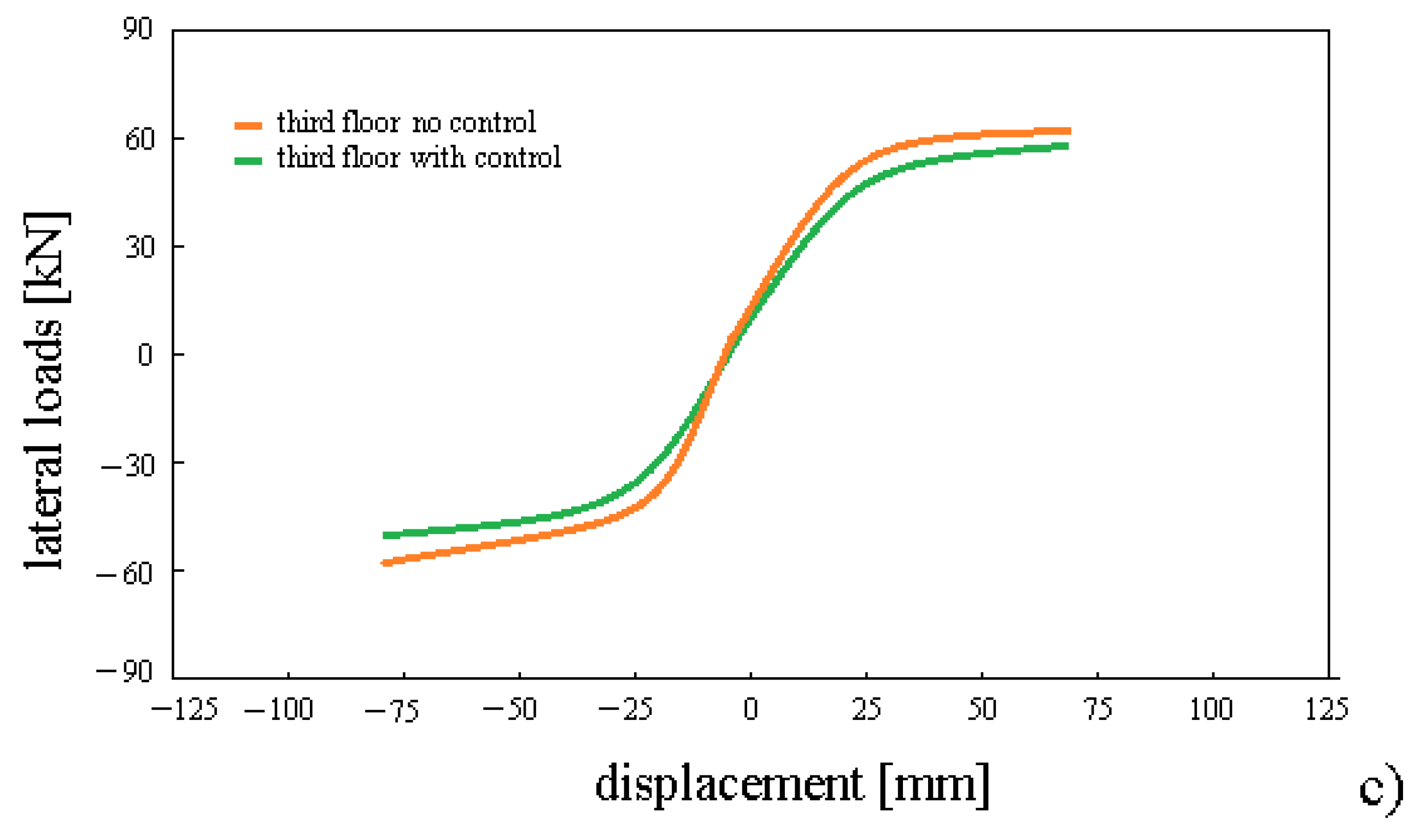
The variation of the lateral loads, with respect to the displacements of each floor, is presented in Figure 4 for $r=1$, for no/with sliding control. We see that the level of displacements is smaller for the sliding control compared to the case without control. The structure is stable and allows displacements within the range $(-75,75)$ mm for $r\le 5$.

To study the behavior of the structure for $r>5$ under sliding control, we computed the Euclidean distance in the phase space between a trajectory and a trajectory obtained by a slight perturbation of this trajectory at $t=0$ as [23]

$$D(t)=\sqrt{{\displaystyle \sum _{i=1}^3{(x_i^0-x_i^1)}^2+{\displaystyle \sum _{i=1}^3{({\dot{x}}_i^0-{\dot{x}}_i^1)}^2{t}^2}}},$$

(22)

where the superscript $0$ indicates a trajectory and $1$ indicates the perturbed trajectory, respectively. For certain values of the ratio $r=F(t)/F_0$, the motion of the structure shows an exponential increase in a short interval of time. This instability made us consider the chaotic motion, which is characterized by the Lyapunov exponent $\overline{\mathsf{\lambda }}$, defined by

$$\exp (\overline{\mathsf{\lambda }}t)={\lim }_{D_{0\to 0}}D(t)/D_0$$

(23)

The variation of $\ln (D(\mathsf{\tau })/D_0)$, with respect to $t$, is presented in Figure 5 for $r\in (5,5.8)$ and $r\in (5.8,7)$. The interpolated lines used to calculate the Lyapunov exponents are marked in red [23]. The variation of $\ln (D(\mathsf{\tau })/D_0)$, with respect to $t$, defines a threshold between the regular and chaotic motions, with respect to $r$. We observe from this figure that the structure admits two Lyapunov exponents, ${\overline{\mathsf{\lambda }}}_1=$0.43 and ${\overline{\mathsf{\lambda }}}_2=$ 0.35. This means that the motion is characterized by two attractors and at least one of which has a tendency towards chaos. This behavior is described in [23,24] for a class of models governed by the Sommerfeld effect and [25] for a Rössler chemical reaction system.

The study of behavior of the structure under seismic loads is strongly related to active and passive control techniques. An enhanced reduced model for elastic earthquake response analysis of a class of mono-symmetric shear building structure with constant eccentricity is analyzed in [26]. The method consists of the construction of a reduced model, with the degrees of freedom at representative floor levels only, and the transformation of earthquake input forces into a set of reduced input forces. We added the self-powered active control and energy regenerated to the power source, discussed in [27]. The impacts of adjustable damping on the motor force and energy consumption were investigated. The results demonstrate the advantages of the hybrid active semiactive suspension in energy conservation with various suspension control objectives.

An adaptive observer for simultaneously estimating the parameters and states in a shear structure is presented in [28]. The energy-dissipation device is illustrated, with experimental results gathered, with a reduced-scale five-story structure with a magneto-rheological damper. Perspectives of further assessment can extend the mentioned technique of calculation to other contexts as the out-of-plane dynamics of masonry walls [29] or the dynamic control of bridges [30].

4. Conclusions

An advantage of the sliding-mode control consists of its stability for dynamic systems subjected to seismic loads. On the negative side, the sliding-mode control use large and rapidly switching control signals, which consume a lot of energy and damage the control actuators.

To overcome this disadvantage, the Ricci flow and the trajectories moving on a manifold were introduced. In this way, we clarified the important ideas behind the sliding mode motion control and the structure response. The sliding-mode control involves selection of a sliding manifold, such that the system trajectory intersects, moves, and stays on this manifold.

The sliding mode control law has the ability to drive trajectories to the sliding motions in a finite period of time. This means that the stability of the sliding manifold is better than the asymptotic stability.

References

- Aldemir, U.; Bakioglu, M.; Akhiev, S.S. Optimal control of linear buildings under seismic excitations. Earthq. Eng. Struct. Dyn. 2001, 30, 835–851. [Google Scholar] [CrossRef]
- Drakunov, S.V.; Utkin, V.I. Sliding mode control in dynamic systems. Int. J. Control 1992, 55, 1029–1037. [Google Scholar] [CrossRef]
- Lynch, J.P.; Law, K.H. Market-based control of linear structural systems. Earthq. Eng. Struct. Dyn. 2002, 31, 1855–1877. [Google Scholar] [CrossRef] [Green Version]
- Edwards, C.; Spurgeon, S.K. Sliding Mode Control; Taylor & Francis Ltd.: Oxfordshire, UK, 1998. [Google Scholar]
- Bhatti, A.I. Advanced Sliding Mode Controllers for Industrial Applications. Ph.D. Thesis, University of Leicester, Leicester, UK, 1998. [Google Scholar]
- Utkin, V.I. Sliding Modes in Control and Optimization; Springer: Berlin/Heidelberg, Germany, 1992. [Google Scholar]
- Utkin, V.I.; Poznyak, A.S. Advances in Sliding Mode Control; Adaptive Sliding Mode Control; Springer: Berlin/Heidelberg, Germany, 2013; pp. 21–53. [Google Scholar]
- Plestan, Y.; Shtessel, V.; Brégeault, V.; Poznyak, A. New methodologies for adaptive sliding mode control. Int. J. Control 2010, 83, 1907–1919. [Google Scholar] [CrossRef] [Green Version]
- Golembo, B.Z.; Yemelyanov, S.V.; Utkin, V.I.; Shubladze, A.M. Application of piecewise-continuous dynamic systems to filtering problems. Autom. Remote Control 1976, 37, 369–377. [Google Scholar]
- Slotine, J.J.; LI, W. Applied Nonlinear Control; Prentice-Hall: Englewood Cliffs, NJ, USA, 2010. [Google Scholar]
- Hamilton, R. The Ricci flow on surfaces. Contemp. Math. 1988, 71, 237–262. [Google Scholar]
- Perelman, G. The entropy formula for the Ricci flow and its geometric applications. arXiv 2003, arXiv:Math.DG/0211159. [Google Scholar]
- Perelman, G. Ricci flow with surgery on three-manifolds. arXiv 2002, arXiv:math.DG/0303109. [Google Scholar]
- Chen, B.-Y. A survey on Ricci solitons on Riemannian submanifolds. Contemp. Math. 2016, 674, 27–39. [Google Scholar]
- Ivey, T. Ricci solitons on compact three-manifolds. Diff. Geom. Appl. 1993, 3, 301–307. [Google Scholar] [CrossRef] [Green Version]
- Ivey, T. New examples of complete Ricci solitons. Proc. Amer. Math. Soc. 1994, 122, 241–245. [Google Scholar] [CrossRef]
- Baird, P.; Danielo, L. Three-dimensional Ricci solitons which project to surfaces. J. Fur Die Reine Und Angew. Math. 2007, 608, 65–91. [Google Scholar] [CrossRef] [Green Version]
- Chiroiu, V.; Munteanu, L.; Bratu, P. Ricci Soliton equation with applications to Zener schematics. In Proceedings of the International Conference Riemannian Geometry and Applications—RIGA 2021, Bucharest, Romania, 15–17 January 2021. [Google Scholar]
- Munteanu, L.; Chiroiu, V.; Bratu, P. On the Ricci soliton equation-Part I. Cnoidal Method. Rom. J. Mech. 2020, 5, 22–42. [Google Scholar]
- Sheridan, N. Hamilton’s Ricci Flow. Ph.D. Thesis, The University of Melbourne, Dept. of Mathematics and Statistics, Parkville, VIC, Australia, 2006. [Google Scholar]
- Cao, H.-D.; Zhu, X.-P. A complete proof of the Poincare and geometrization conjectures—Application of the Hamilton-Perelman theory of the Ricci flow. Asian J. Math. 2006, 10, 165–492. [Google Scholar] [CrossRef] [Green Version]
- Hung, J.Y.; Gao, W.; Hung, J.C. Variable Structure Control: A Survey. IEEE Trans. Ind. Electron. 1993, 40, 2–21. [Google Scholar] [CrossRef] [Green Version]
- Munteanu, L.; Chiroiu, V.; Sireteanu, T. On the response of small buildings to vibrations. Nonlinear Dyn. 2013, 73, 1527–1543. [Google Scholar] [CrossRef]
- Munteanu, L.; Brişan, C.; Chiroiu, V.; Dumitriu, D.; Ioan, R. Chaos-hyperchaos transition in a class of models governed by Sommerfeld effect. Nonlinear Dyn. 2014, 78, 1877–1889. [Google Scholar] [CrossRef]
- Yanchuk, S.; Kapitaniak, T. Chaos-hyperchaos transition in coupled Rossler systems. Physics Lett. A 2001, 290, 139–144. [Google Scholar] [CrossRef]
- Adachi, F.; Yoshitomi, S.; Tsuji, M.; Takewaki, I. Enhanced reduced model for elastic earthquake response analysis of a class of mono-symmetric shear building structures with constant eccentricity. Soil Dyn. Earthq. Eng. 2011, 31, 1040–1050. [Google Scholar] [CrossRef] [Green Version]
- Chen, L.; Shi, D.; Wang, R.; Zhou, H. Energy Conservation Analysis and Control of Hybrid Active Semiactive Suspension with Three Regulating Damping Levels. Shock Vib. Vol. 2016. [Google Scholar] [CrossRef] [Green Version]
- Jiménez-Fabián, R.; Alvarez-Icaza, L. An adaptive observer for a shear building with an energy-dissipation device. Control Eng. Practice 2010, 18, 331–338. [Google Scholar] [CrossRef]
- Solarino, F.; Giresini, L.; Oliveira, D.V. Mitigation of amplified response of restrained rocking walls through horizontal dampers. In Proceedings of the 11th International Conference on Structural Dynamic EURODYN, Athens, Greece, 23–26 November 2020; Volume 2, pp. 4292–4303. [Google Scholar]
- Stochino, F.; Fadda, M.L.; Mistretta, F. Assessment of RC bridges integrity by means of low-cost investigations. Frat. Integrita Strutt. 2018, 12, 216–225. [Google Scholar] [CrossRef] [Green Version]
Figure 1.
Model for the three-story building.
Figure 2.
Geodesics in a two-manifold of positive or negative curvature.
Figure 3.
Ground acceleration used to excite the model.
Figure 4.
Lateral loads versus displacements in the structure with no/with sliding control; (a) first floor; (b) second floor, (c) third floor.
Figure 5.
Time dependence of for and .
Publisher’s Note: MDPI stays neutral with regard to jurisdictional claims in published maps and institutional affiliations. |
© 2021 by the authors. Licensee MDPI, Basel, Switzerland. This article is an open access article distributed under the terms and conditions of the Creative Commons Attribution (CC BY) license (http://creativecommons.org/licenses/by/4.0/).
Share and Cite
MDPI and ACS Style
Munteanu, L.; Dumitriu, D.; Brisan, C.; Bara, M.; Chiroiu, V.; Nedelcu, N.; Rugina, C. Sliding Mode Control and Geometrization Conjecture in Seismic Response. Symmetry 2021, 13, 353. https://0-doi-org.brum.beds.ac.uk/10.3390/sym13020353
AMA Style
Munteanu L, Dumitriu D, Brisan C, Bara M, Chiroiu V, Nedelcu N, Rugina C. Sliding Mode Control and Geometrization Conjecture in Seismic Response. Symmetry. 2021; 13(2):353. https://0-doi-org.brum.beds.ac.uk/10.3390/sym13020353
Chicago/Turabian StyleMunteanu, Ligia, Dan Dumitriu, Cornel Brisan, Mircea Bara, Veturia Chiroiu, Nicoleta Nedelcu, and Cristian Rugina. 2021. "Sliding Mode Control and Geometrization Conjecture in Seismic Response" Symmetry 13, no. 2: 353. https://0-doi-org.brum.beds.ac.uk/10.3390/sym13020353
Note that from the first issue of 2016, this journal uses article numbers instead of page numbers. See further details here.