
Application of the Efros Theorem to the Function Represented by the Inverse Laplace Transform of s−μ exp(−sν)


1
Department of Chemical Engineering, Ben Gurion University of the Negev, Beer Sheva 84105, Israel
2
Dipartimento di Fisica e Astronomia, Università di Bologna, Via Irnerio 46, I-40126 Bologna, Italy
*
Author to whom correspondence should be addressed.
Symmetry 2021, 13(2), 354; https://0-doi-org.brum.beds.ac.uk/10.3390/sym13020354
Submission received: 31 January 2021
/
Revised: 10 February 2021
/
Accepted: 14 February 2021
/
Published: 22 February 2021
(This article belongs to the Special Issue Special Functions and Polynomials)
Abstract
:Using a special case of the Efros theorem which was derived by Wlodarski, and operational calculus, it was possible to derive many infinite integrals, finite integrals and integral identities for the function represented by the inverse Laplace transform. The integral identities are mainly in terms of convolution integrals with the Mittag–Leffler and Volterra functions. The integrands of determined integrals include elementary functions (power, exponential, logarithmic, trigonometric and hyperbolic functions) and the error functions, the Mittag–Leffler functions and the Volterra functions. Some properties of the inverse Laplace transform of with and are presented.
Keywords:
efros theorem; inverse laplace transforms; wright functions; Mittag–Leffler functions; volterra functions; modified bessel functions; finite; infinite and convolution integralsMSC:
26A33; 33C10; 33E12; 34A25; 44A201. Introduction
Inversions of the Laplace transforms of exponential functions
were during the 1945–1970 period in a focus of attention of a number of well-known mathematicians like Humbert [1], Pollard [2], Wlodarski [3], Mikusinski [4,5,6,7], Wintner [8], Ragab [9] and Stankovič [10]. In the case , Mikusinski was able to obtain the inverse Laplace transform in terms of integral representations [7]
and also as the finite trigonometric integral
It was established that the functions can be expressed in terms of exponential and parabolic cylinder functions when [9,11] and by help of the Airy functions and their first derivatives for and [9,12]. For , the solution was deduced by Barkai [13] in 2001 using Mathematica as a sum of three generalized hypergeometric functions, but the numerical result was uncertain, presumably for a bag in the computing program. In 2010–2012 Gorska and Penson [14,15] were able to represent in terms of Mejer G functions. Earlier, in 1958 Ragab [9] expressed in terms of MacRobert E functions for .
In 1952 Wlodarski [3] showed that when the generalized product Efros theorem [16] is applied to the Laplace transform of which is given in (1), then it is possible to derive the following formula
It was established in our recent paper [17] that for and this functional expression can be written in terms of specific Wright functions , sometimes referred to as the Mainardi functions
in the following way
This follows from the fact that the functions and satisfy
It was also illustrated by us in [17], that in many cases, by using standard tables of the Laplace transforms [18,19,20,21], the left hand side Laplace transforms in (6) can be inverted and numerous infinite integrals, finite integrals and integral identities for the functions and can be derived.
Let us recall that the Wright functions [22,23], considered initially as a some kind generalization of the Bessel functions, are defined as an entire functions of the argument and parameters and by
It is usual to distinguish them in two kinds, the first kind with and the second kind with and , see, e.g., [11].
Restricting our attention to positive argument , the Mainardi functions turn out to be particular Wright functions of the second kind expressed by the following series
The interest in the Wright functions of the second kind comes from the fact that they play an important role in solution of the linear partial differential equations of fractional order which describe a wide spectrum of phenomena including probability distributions, anomalous diffusion and diffusive waves [24,25,26,27,28,29,30,31,32,33].
In Section 2, of this paper, by using the complex inversion formula in (1) and the Bromwich contour, the integral representation of with and is derived and some basic properties of this inverse transform are established. The cases can be dealt as well, see Appendix A for details.
The next two Section 3 and Section 4 are devoted to evaluation of infinite, finite and convolution integrals by using the Efros theorem in the Wlodarski form. The integrands of these integrals or integral identities include the elementary functions (power, exponential, logarithmic, trigonometric and hyperbolic functions) and the special functions (the error function, Mittag–Leffler functions and the Volterra functions). The last section provides concluding remarks.
In derivations of these integrals direct and inverse Laplace transforms which are taken from tables of transforms [18,19,20,21] are always presented in mathematical expressions. All mathematical operations and manipulations with elementary and special functions, integrals and transforms are formal and their validity is assured by considering the restrictions usually imposed in the operational calculus.
2. Integral Representations of the Inverse Laplace Transform of
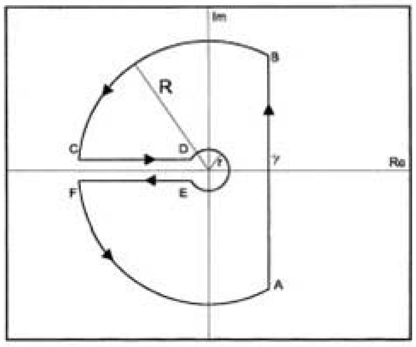
Before infinite integrals in (6) will be evaluated, it is of interest to derive the function by performing the complex integration from (1). In investigated case, the branch point of the integrand exists and is located at the origin and therefore the equivalent Bromwich contour is plotted in Figure 1. The closed contour of integration ABCDEFA includes the line AB, the arcs BC and FA of a circle of radius with center at origin, the arc DE of a circle of radius with center at origin, and two parallel lines CD and EF. The the cut along the negative axis ensures that is a single-valued function. However, according to the Cauchy lemma the integrals along the arcs BC and FA vanish as .
As a consequence there are only three contributions coming from integrals on the CD and EF lines and from the small circle round origin, DE, so we have
However, the last trigonometric integral vanishes for and therefore the final result of the complex integration from (10) is
The same integral representation has been derived in 1970 by Stankoviċ [10] for the Wright function, but on the negative values of the argument t and which is presented here in our notation
and comparing (11) with (12) we have that the inverse exponential functions can be expressed in terms of the Wright functions, in agreement with the survey analysis by Mainardi and Consiglio [33] where also plots are presented,
In particular, for the Wright functions are reduced to the Mainardi functions and [11]
For and , the integrals in (11) become the Laplace transforms of trigonometric functions [18,19,20,21]
Differentiation of the integral (11) with respect to the argument t gives
and using rules of the operational calculus we have the initial and final values of the function from [33]
This is in an agreement with the finding of Pollard [2] that for , the inverse Laplace transform is positive almost everywhere, but for Stankoviċ [10] postulated that in a some interval this function is negative and has at least one zero. Expanding the exponent in into series it is possible to obtain the behaviour of the function for large values of the argument t
The integral of the can be derived directly from
In order to obtain the recurrence relations the following operational rule can be applied
and the inverse transforms in (22) are
3. Integrals of the Inverse Laplace Transform of with Elementary Functions
In the first example the Wlodarski integral formula (4) is applied to the power function ,
and therefore we have
The above results can be extended to functions which are defined at finite intervals and to step functions jumping at integral values of variable t. Let start with
which leads to the finite integral
In the next example, from
we have
Using
it is possible to derive
In the next example the case of exponential function is considered:
By changing variable of integration , all convolution integrals can be expressed as in terms of finite trigonometric integrals. The shifted increasing and decreasing exponential functions are considered in the following two examples. From
we have the convolution of two functions.
Similarly from
it is possible to obtain
The logarithmic functions are the next group of elementary functions to be considered. In the simplest case from
where is the Euler constant, it follows that
In the more general case
we have
Trigonometric and hyperbolic functions is the last groups of elementary functions to be considered. From:
the following integral identity is derived
Similarly as in (45), for the hyperbolic sine function, the change is only in the sign
and therefore we have
In the case of cosine function, from;
we have
In the case of the product of trigonometric and hyperbolic sine functions the direct and inverse Laplace transforms are
and therefore
For the product of trigonometric and hyperbolic sine functions we have
and therefore
4. Integrals of the Inverse Laplace Transform of with the Mitag-Leffler, Error and Volterra Functions
The Laplace transform of the two parameter Mittag–Leffler function is [11,34,35,36]
and this permits to obtain
and
Thus, in both sides of expressions (59) appear the Mittag–Leffler functions. Evidently, for they are reduced to the classical Mittag–Leffler functions.
and for and we have
If , in the integrands of (61) the Mittag–Leffler functions are expressed then by the error functions [35,36]
If is positive integer, the Mittag–Leffler functions are expressed by elementary functions [36]. In particular cases, with . and the explicit form of the inverse transforms of exponential functions is known (see (15) and (17)).
The Laplace transform of the error function is
which yields
The Volterra functions are defined by the following integrals [37]:
and their Laplace transforms are
The logarithmic functions in the Laplace transforms permit to express the integrals of the Volterra functions with inverse Laplace transform of exponential function in terms of convolution integrals. From
it follows that
Similarly from
we have
The number of similar convolution integrals can be significantly enlarged if the Volterra functions are multiplied by with , then their Laplace transforms should be differentiated n times. The result of such differentiations are linear combinations of these functions [34,35,36]. For example, with and we have
5. Conclusions
By applying the Efros theorem in the form established by Wlodarski it was possible to derive a number of infinite integrals, finite integrals and integral identities with the function which represent the Laplace inverse transform of with and . The extension to the cases is dealt in Appendix A Derived by us integrals include in integrands elementary functions (power, exponential, logarithmic, trigonometric and hyperbolic functions) and the error functions, the Mittag–Leffler functions and the Volterra functions. Many results appear in form of the convolution integrals. Performing the inversion by the complex integration, it was possible to show that the inverse Laplace inverse transform, which means the original function, can be also expressed in terms of the Wright functions and for particular values of parameters by the Mainardi functions. Using rules of operational calculus some properties of the inverse Laplace transform were derived.
Author Contributions
These authors contributed equally to this work. All authors have read and agreed to the published version of the manuscript.
Funding
This research received no external funding.
Acknowledgments
The research work of F.M. has been carried out in the framework of the activities of the National Group of Mathematical Physics (GNFM, INdAM). Both the authors would like to acknowledge the unknown reviewers for their constrictive comments.
Conflicts of Interest
The authors declare no conflict of interest.
Appendix A. Additional Properties of the Inverse of the Laplace Transform of
The restriction posed on the second parameter of the function , i.e., (in the inverse of the Laplace transform ) can be removed by using rules of operational calculus. In the general case, for a non-negative parameter , this inverse transform can always be expressed as the convolution integral which includes the corresponding power function:
In the particular case , it reduces to the simple integral, because expresses the integration operation:
The product of two identical or different Laplace inverse transforms can be derived in the form of convolution integrals from
which gives
These results can be generalized to n-fold integrals when exists the factor , with .
In the case of the product of identical Laplace inverse transforms it is reduced to the following convolution integral
In similar way, if the inverse transform is in a more general form with ,
we have
The differentiation of Laplace inverse transforms with respect to the parameters and gives
which yields the following inverses of (A8)
where denotes the Euler constant.
References
- Humbert, P. Nouvelle correspondances symboliques. Bull. Soc. Math. 1945, 69, 121–129. [Google Scholar]
- Pollard, H. The representation of exp(−xλ) as a Laplace integral. Bull. Am. Math. Soc. 1946, 52, 908–910. [Google Scholar] [CrossRef] [Green Version]
- Wlodarski, L. Sur une formule de Eftros. Stud. Math. 1952, 13, 183–187. [Google Scholar] [CrossRef] [Green Version]
- Mikusinski, J. Sur les fonctions exponentielles du calcul opératoire. Stud. Math. 1951, 12, 208–224. [Google Scholar] [CrossRef]
- Mikusinski, J. Sur la croissance de la function opérationelle exp(−sαλ). Bull. Acad. Polon. 1953, 4, 423–425. [Google Scholar]
- Mikusinski, J. Sur la function dont la transformée de Laplace est exp(−sαλ). Bull. Acad. Polon. 1958, 6, 691–693. [Google Scholar]
- Mikusinski, J. On the function whose Laplace transform is exp(−sλ). Stud. Math. 1959, 18, 195–198. [Google Scholar] [CrossRef] [Green Version]
- Wintner, A. Cauchy’s stable distributions and an “explicit formula” of Mellin. Am. J. Math. 1956, 78, 819–861. [Google Scholar] [CrossRef]
- Ragab, F.M. The inverse Laplace transform of a exponential function. Comm. Pure Appl. Math. 1958, 11, 115–127. [Google Scholar] [CrossRef]
- Stankovič, B. On the function of E.M. Wright. Publications de L’Institute Mathématique. Nouvelle Série 1970, 10, 113–124. [Google Scholar]
- Mainardi, F. Fractional Calculus and Waves in Linear Viscoelasticity; Imperial College Press: London, UK, 2010. [Google Scholar]
- Hanyga, A. Multidimensional solutions of time-fractional diffusion-wave equations. Proc. R. Soc. A 2002, 458, 933–957. [Google Scholar] [CrossRef]
- Barkai, E. Fractional Fokker-Planck equation, solution, and application. Phys. Rev. E 2001, 63, 046118. [Google Scholar] [CrossRef] [Green Version]
- Penson, K.A.; Górska, K. Exact and explicit probability densities for one-sided Lévy stable distribution. Phys. Rev. Lett. 2010, 105, 210604. [Google Scholar] [CrossRef] [Green Version]
- Górska, K.; Penson, K.A. Lévy stable distributions via associated integral transform. J. Math. Phys. 2012, 53, 053302. [Google Scholar] [CrossRef] [Green Version]
- Efros, A.M. Some applications of operational calculus in analysis. Mat. Sb. 1935, 42, 699–705. [Google Scholar]
- Apelblat, A.; Mainardi, F. Application of the Efros theorem to the Wright functions of the second kind and other results. Lect. Notes TICMI 2020, 21, 9–28. [Google Scholar]
- Erdélyi, A.; Magnus, W.; Oberhettinger, F.; Tricomi, F.G. Tables of Integral Transforms; McGraw-Hill: New York, NY, USA, 1954. [Google Scholar]
- Roberts, G.E.; Kaufman, H. Tables of Laplace Transforms; W.B. Saunders Co.: Philadelphia, PA, USA, 1966. [Google Scholar]
- Hladik, J. La Transformation de Laplace a Plusieurs Variables; Masson et Cie Éditeurs: Paris, France, 1969. [Google Scholar]
- Oberhettinger, F.; Badii, L. Tables of Laplace Transforms; Springer: Berlin, Germany, 1973. [Google Scholar]
- Wright, E.M. On the coefficients of power series having exponential singularities. Lond. Math. Soc. 1933, 8, 71–79. [Google Scholar] [CrossRef]
- Wright, E.M. The generalized Bessel function of order greater than one. Quart. J. Math. 1940, 11, 36–48. [Google Scholar] [CrossRef]
- Montroll, E.W.; Bendler, J.T. On Lévy (or stable) distributions and the Williams-Watts model of dielectric relaxation. J. Stat. Phys. 1984, 34, 129–192. [Google Scholar] [CrossRef]
- Zolotarev, V.M. One-dimensional Stable Distributions. Translated from Russian by H.H. McFaden. Am. Math. Soc. 1986. [Google Scholar]
- Mainardi, F. On the initial value problem for the fractional diffusion-wave equation. In Proceedings of the 7th Conference on Waves and Stability in Continuous Media (WASCOM 1993), Bologna, Italy, 4–9 October 1993; Rionero, S., Ruggeri, T., Eds.; World Scientific: Singapore, 1994; pp. 246–251. [Google Scholar]
- Saichev, A.I.; Zaslavsky, G.M. Fractional kinetic equations: Solutions and applications. Chaos 1997, 7, 753–764. [Google Scholar] [CrossRef] [PubMed] [Green Version]
- Mainardi, F.; Tomirotti, M. Seismitic pulse propagation with constant Q and stable probability distributions. Ann. Geofis. 1997, 40, 1311–1328. [Google Scholar]
- Gorenflo, R.; Luchko, Y.; Mainardi, F. Analytical properties and applications of the Wright functions. Fract. Calc. Appl. Anal. 1999, 2, 383–414. [Google Scholar]
- Mainardi, F.; Luchko, Y.; Pagnini, G. The fundamental solution of the space-time fractional diffusion equation. Fract. Calc. Appl. Anal. 2001, 4, 153–192. [Google Scholar]
- Mainardi, F.; Mura, A.; Pagnini, G.; Gorenflo, R. Fractional relaxation and time- fractional diffusion of distributed order. In Proceedings of the 2ND IFAC Workshop on Fractional Differentiation and its Applications, Porto, Portugal, 19–21 July 2006. [Google Scholar]
- Garg, M.; Rao, A. Fractional extensions of some boundary value problems in oil strata. Proc. India Acad. Sci. (Math. Sci.) 2007, 117, 267–281. [Google Scholar] [CrossRef] [Green Version]
- Mainardi, F.; Consiglio, A. The Wright functions of the second kind in Mathematical Physics. Mathematics 2020, 8, 884. [Google Scholar] [CrossRef]
- Apelblat, A. Laplace Transforms and Their Applications; Nova Science Publishers, Inc.: New York, NY, USA, 2012. [Google Scholar]
- Apelblat, A. Differentiation of the Mittag–Leffler functions with respect to parameters in the Laplace transform approach. Mathematics 2020, 8, 657. [Google Scholar] [CrossRef]
- Gorenflo, R.; Kilbas, A.A.; Mainardi, F.; Rogosin, S.V. Mittag–Leffler Functions, Related Topics and Applications, 2nd ed.; Springer: Berlin/Heidelberg, Germany, 2020. [Google Scholar]
- Apelblat, A. Volterra Functions; Nova Science Publishers, Inc.: New York, NY, USA, 2008. [Google Scholar]
Figure 1.
The equivalent Bromwich contour.

Publisher’s Note: MDPI stays neutral with regard to jurisdictional claims in published maps and institutional affiliations. |
© 2021 by the authors. Licensee MDPI, Basel, Switzerland. This article is an open access article distributed under the terms and conditions of the Creative Commons Attribution (CC BY) license (http://creativecommons.org/licenses/by/4.0/).
Share and Cite
MDPI and ACS Style
Apelblat, A.; Mainardi, F. Application of the Efros Theorem to the Function Represented by the Inverse Laplace Transform of s−μ exp(−sν). Symmetry 2021, 13, 354. https://0-doi-org.brum.beds.ac.uk/10.3390/sym13020354
AMA Style
Apelblat A, Mainardi F. Application of the Efros Theorem to the Function Represented by the Inverse Laplace Transform of s−μ exp(−sν). Symmetry. 2021; 13(2):354. https://0-doi-org.brum.beds.ac.uk/10.3390/sym13020354
Chicago/Turabian StyleApelblat, Alexander, and Francesco Mainardi. 2021. "Application of the Efros Theorem to the Function Represented by the Inverse Laplace Transform of s−μ exp(−sν)" Symmetry 13, no. 2: 354. https://0-doi-org.brum.beds.ac.uk/10.3390/sym13020354
Note that from the first issue of 2016, this journal uses article numbers instead of page numbers. See further details here.