GLM-Based Flexible Monitoring Methods: An Application to Real-Time Highway Safety Surveillance

Abstract

Statistical modeling of historical crash data can provide essential insights to safety managers for proactive highway safety management. While numerous studies have contributed to the advancement from the statistical methodological front, minimal research efforts have been dedicated to real-time monitoring of highway safety situations. This study advocates the use of statistical monitoring methods for real-time highway safety surveillance using three years of crash data for rural highways in Saudi Arabia. First, three well-known count data models (Poisson, negative binomial, and Conway–Maxwell–Poisson) are applied to identify the best fit model for the number of crashes. Conway–Maxwell–Poisson was identified as the best fit model, which was used to find the significant explanatory variables for the number of crashes. The results revealed that the road type and road surface conditions significantly contribute to the number of crashes. From the perspective of real-time highway safety monitoring, generalized linear model (GLM)-based exponentially weighted moving average (EWMA) and cumulative sum (CUSUM) control charts are proposed using the randomized quantile residuals and deviance residuals of Conway–Maxwell (COM)–Poisson regression. A detailed simulation-based study is designed for predictive performance evaluation of the proposed control charts with existing counterparts (i.e., Shewhart charts) in terms of the run-length properties. The study results showed that the EWMA type control charts have better detection ability compared with the CUSUM type and Shewhart control charts under small and/or moderate shift sizes. Finally, the proposed monitoring methods are successfully implemented on actual traffic crash data to highlight the efficacy of the proposed methods. The outcome of this study could provide the analysts with insights to plan sound policy recommendations for achieving desired safety goals.

1. Introduction

Traffic collisions account for over 1.35 million annual fatalities and approximately 50 million injuries worldwide, and are predicted to become the fifth leading cause of death by the year 2030 [1]. On average, road traffic crashes account for approximately 3% of nations’ gross domestic product (GDP) worldwide, irrespective of their growth and rate of motorization [2,3]. Road traffic injuries are the third leading cause of death in Saudi Arabia, which poses a major socio-economic and public health concern for road safety agencies. The country has witnessed rapid economic growth and motorization, particularly after the oil boom in the early 1970s [4,5]. The fatality index (deaths/100,000 population) due to traffic crashes in Saudi Arabia is estimated to be around 27.4, which is significantly high compared with developed countries like the United States, Australia, Sweden, Netherland, the United Kingdom, and the neighboring Gulf states [1]. The average crash to injury ratios of 8:4 and 8:6 reported for different regions in Saudi Arabia are also significantly high compared with the global ratio of 8:1 [6,7]. Several studies have investigated the crash causation factors in Saudi Arabia and neighboring Gulf countries in recent years. Al Kaaf and Abdel-Aty [8] investigated the risk factors for crash occurrence on urban four-lane divided roadway segments in Riyadh, Saudi Arabia. Factors such as annual average daily traffic, speed limit, segment length, and driveway density were found to increase the likelihood of fatal and injury crashes. Islam et al. [9] utilized panel regression models and pooled ordinary least square methods to analyze ten years (2003–2013) of annual crash data from 13 provinces in Saudi Arabia. The study results showed that adverse weather conditions, sandstorms, and the number of vehicles involved were identified as statistically significant for traffic crashes in the country. Poor roadway conditions, road geometry, and tires burst due to intense pavement temperature during summer were also identified as the most common causes of traffic crashes in Saudi Arabia [10,11,12]. Driver distractions, speeding, and non-compliance to traffic rules are among the other predominant causes of traffic crashes in Saudi Arabia [13,14]. Studies conducted by Al-Kheder and Al-Rashidi [15] and Mohamed et al. [16] for neighboring Gulf state Abu Dhabi in United Arab Emirates (UAE) also reported that factors responsible for increased traffic crashes include road type, road surface conditions, excessive speeds, and non-compliance to traffic rules. A generalized linear model (GLM)-based safety appraisal study conducted for Salalah City in Oman also indicated that road geometry and traffic variables (volumes and 85th percentile speed) were the most significant variables affecting the frequency of crashes [17]. Recently, some safety measures and policies have been initiated; however, the situations seem to have marginally improved. Concrete and authentic research is required to explore key risk factors for crash occurrence and severity.

Over the years, researchers have constantly sought various approaches with an aim to gain a better understanding of factors affecting crash occurrences to suggest appropriate countermeasures, and provide directions for policies to improve road safety [18,19,20,21,22,23,24,25,26]. However, road traffic crashes are complex events involving a large number of factors having multi-faceted interactions, making it very challenging to comprehend them fully. Traffic crashes are the outcomes of several contributing factors such as driver attributes, vehicle factors, traffic exposure, roadway geometric features, spatial attributes of surrounding built environment, lighting and weather conditions, and so forth [25,27,28,29]. Among driver’s attributes, distracted driving and speeding are reported to be the leading factors causing increased motor vehicle crashes [30,31,32,33,34,35,36]. Similarly, the likelihood of crash occurrences along the rural multi-lane highway is increased in the presence of a steep roadway gradient, sharp horizontal curve, and acute curve deflection angle [37,38]. Contrarily, lower crash occurrences on the same facilities are associated with the decrease in curve length and horizontal curve radius and an increase in the degree of curvature and number of lanes [20,39]. Likewise, poor road surface conditions, nighttime travel, adverse weather, and precipitation are reported to have a strong bearing on high crash frequencies [40,41,42,43]. A better understanding of all of these factors associated with traffic crashes is essential to promote and enhance the safety performance of road traffic systems. Advances on the methodological front for highway safety research continue to be investigated.

The GLM-based Poisson regression model has been widely proposed to model the equi-dispersed crash frequency data. Poisson models outperform the standard regression approaches in handling random, non-negative sporadic, and discrete features of crash counts. However, crash data are frequently characterized by relatively large sample variance compared with the sample mean, which limits the application of Poisson regression [44]. Therefore, a negative binomial or Poisson gamma regression model is preferred for such datasets that account for the over-dispersion issue, while the GLM-based binomial regression model is often used to fit under-dispersed data. In practice, it is challenging to differentiate the characteristics of data. However, there exist a few standard testing procedures to differentiate the data characteristics. However, the mentioned procedures require excellent expertise, high computational efforts, and time. The Conway–Maxwell (COM)–Poisson (COM–Poisson) model proposed by Guikema and Goffelt [45] is the better alternative, which is a flexible model and able to handle any type of disperse data [46]. Lord et al. [47] and Lord et al. [48] have successfully used COM–Poisson regression to model the traffic crash data.

In the literature, studies have mostly focused on statistical modeling of the traffic crash data. However, factors contributing to crash occurrences and frequency exhibit spatial heterogeneity and vary from one location to another. In an effort to achieve better surveillance of highway safety, large amounts of data are collected by road safety organizations worldwide. Traditionally, the majority of existing crash prediction models rely on aggregated information with relatively large time-scales, usually on a yearly basis. However, researchers have argued that the likelihood of crash potential is significantly influenced by short-term fluctuations in crash contributing factors such as traffic, weather, complex terrains, and so on. Crash frequency models developed using aggregated data are designed to yield the prediction results on average data over a more extended period of time that may lead to loss of potentially useful information about some important explanatory variables. They also result in an error due to unobserved heterogeneity. Therefore, it is crucial to investigate the disaggregate models, also known as real-time crash risk evaluation models, for estimating crash potential in smaller time-scales such as an hour, a day, or a week. Crash prediction models with more refined time-scales are useful as they lead to timely and better safety decisions to improve highway safety. To fill this research gap, this study proposes the application of the statistical process control (SPC) method for real-time monitoring of crash data in the Kingdom of Saudi Arabia. A control chart is a well-known tool for statistical process control (SPC), which is often used to detect abrupt changes in the data [49]. There exist several GLM-based control charts, which are designed on the residuals estimated through GLM modeling. For example, GLM-based control charts based on the Poisson model were proposed by Skinner et al. [50] and Asgari et al. [51] in their studies. Skinner et al. [50] and Jearkpaporn et al. [52] discussed GLM-based control charts based on the Gamma model, while a chart based on the binomial model was proposed by Shang et al. [53] and Amiri et al. [54]. The GLM-based control charts under the negative binomial model were discussed by Alencar et al. [55] and Urbieta et al. [56]. In their study, Kinat et al. [57,58] proposed GLM-based control charts by assuming an inverse Gaussian distributed response variable, while Mahmood [59] proposed GLM-based control charts under the zero-inflated models.

Recently, Park et al. [60] and Park et al. [61] proposed Shewhart type GLM-based control charts by assuming the COM–Poisson distributed response variable. Park et al. [60] considered deviance residuals as the plotting statistics, while in another study, the authors utilized randomized quantile residuals as the plotting statistics. In general, the Shewhart type charts are designed based on the current information, and they are used to detect a large deviation from the mean of data. Practitioners are usually interested in detecting small changes as early as possible, for which exponentially weighted moving average (EWMA) and cumulative sum (CUSUM) are especially designed structures. Both EWMA and CUSUM charts are designed based on past and current information, which makes them more efficient to detect small or/and moderate shifts in the process mean. This study intends to design EWMA and CUSUM type GLM-based control charts using the deviance and randomized quantile residuals of the COM–Poisson regression model. Further, the performance evaluation and comparative analysis are conducted using the simulated data, and the proposed methods are implemented to monitor the number of crashes reported in Saudi Arabia.

The remainder of this paper is structured as follows. Section 2 presents a description of the data utilized in the current study. Section 3 highlights the proposed research methodology for crash frequency modeling and statistical process monitoring. Section 4 provides a comparative study of the proposed control charts using an extensive simulation study. Section 5 presents the implementation of proposed methods on the traffic collisions data. Finally, Section 6 summarizes key findings, study limitations, and outlook for future research.

2. Data Description

Motor vehicle crash data used in this study were procured from the ministry of transport, Riyadh, Saudi Arabia. A total of 47,984 crashes were reported during the three years (January 2017 to December 2019) of the study period. The study is focused explicitly on crashes involving only motor vehicles along inter-cities rural highways that fall under the ministry of transport jurisdiction. A significant proportion of these highways in the study area run through plain and desert terrain, having warm to high temperatures during most part of the year. Road inventory data are collected from the ministry for available sections, and for others, the geographic information system (GIS) tool was used to extract roadway geometric features. Each crash comprises several explanatory variables (shown in

Table 1. Descriptive statistics of explanatory variables.

Code	Description	Frequency	Percentage	Mean ± S.E
Road Type
1	Divided Highway	17,064	35.56	1.873 ± 0.141
2	Expressway	20,196	42.09
3	Single Highway	10,724	22.35
Road Surface Conditions
1	Cracks and Fossils	8	0.00017	1.840 ± 0.325
2	Dry	2	0.00004
3	Good	28,824	0.60070
4	Maintenance on Road	34	0.00071
5	Others	19,111	0.39828
6	Sand	2	0.00004
7	Wet	3	0.00006
Reported Damage Road Type
1	Barrier	4632	9.65	4.489 ± 0.232
2	Signboard	799	1.67
3	Fence	1649	3.44
4	Lighting Poles	608	1.27
5	No Damage	40,296	83.98
Weather Conditions
1	Dusty	531	0.011066	3.002 ± 0.145
2	Fog	251	0.005231
3	Shiny	45,063	0.939126
4	Others	648	0.013505
5	Rainy	1491	0.031073
Road Markings (Dummy variable, 1 = yes, 0 = no)
0	Present	47,413	98.81	0.989 ± 0.027
1	Absent	571	1.19
Road Cat eyes (Dummy variable, 1 = yes, 0 = no)
0	Present	47,382	98.75	$0.988\pm 0.031$
1	Absent	602	1.25

), including road type, road surface conditions at those sites, damage type post-crash, weather conditions, and presence or absence of road markings and cat eyes.

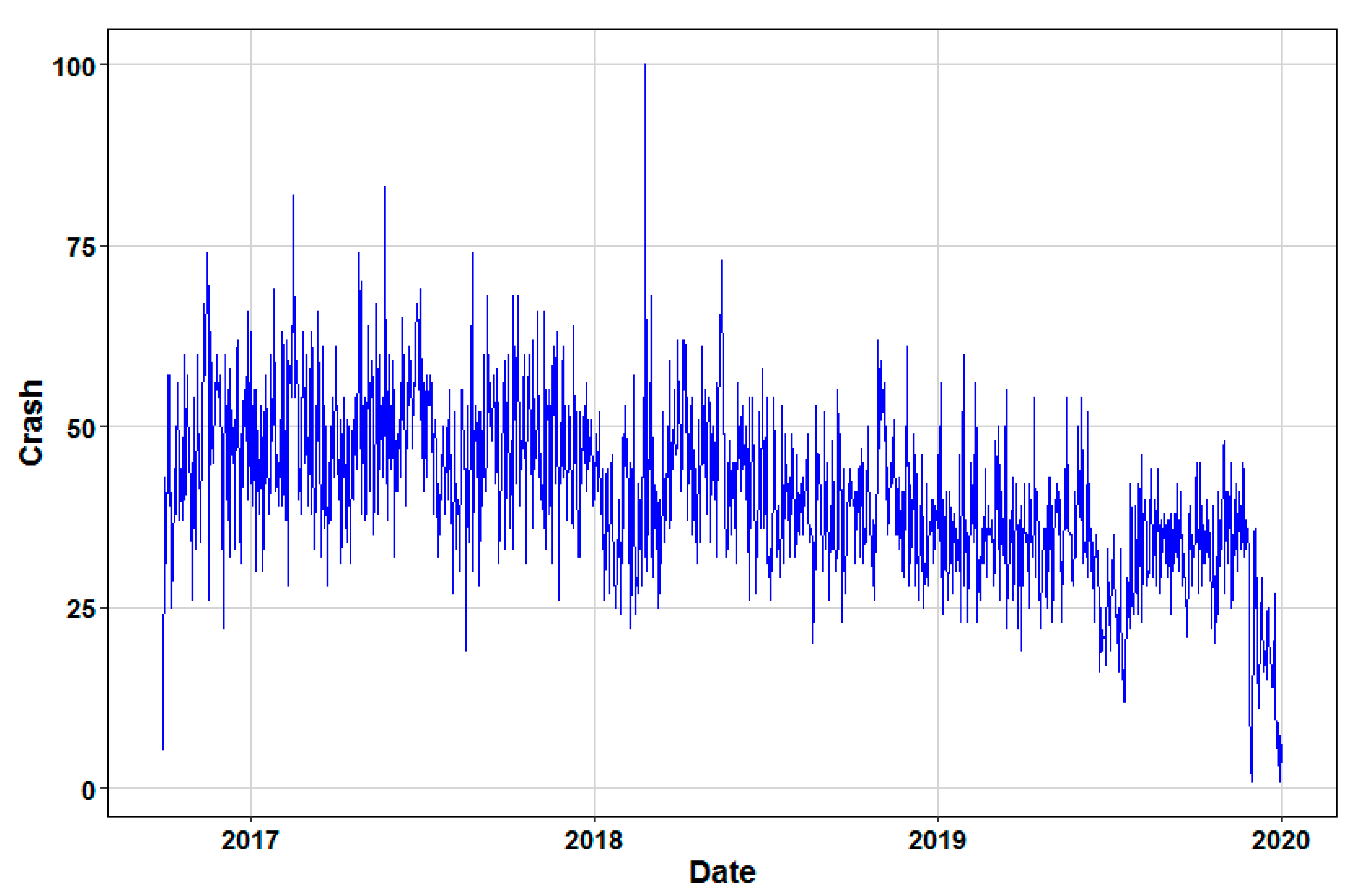
In this study, frequency-based modeling was carried out for crashes aggregated on a daily basis. Figure 1 shows a time series plot of aggregated daily count data of the number of crashes. To access the best-fitting distribution of the aggregated crashes, we have implemented three well-known count models, i.e., Poisson, negative binomial, and COM–Poisson. The detailed diagnostic analysis and model estimation results (shown in

Table 2. Diagnosis analysis of best-fitted distribution for aggregated crashes. AIC, Akaike information criteria; BIC, Bayesian information criteria; COM, Conway–Maxwell.

	Poisson	Negative Binomial	COM–Poisson
Parameter(s)	$\widehat{\lambda }=40.90 \left(0.19\right)$	$\widehat{n}=15.43\left(0.90\right)$	$\widehat{\lambda }=2.78 \left(0.12\right)$
		$\widehat{\mu }=40.90\left(0.35\right)$	$\widehat{\nu }=0.28 \left(0.01\right)$
Loglikelihood	−5367.76	−4651.99	−4618.6
AIC	10,737.53	9307.99	9241.16
BIC	10742.6	9318.15	9251.32

) indicate that COM–Poisson distribution is the best-fitting model as it produced the minimum values of decision criteria (i.e., loglikelihood, Akaike information criteria (AIC), and Bayesian information criteria (BIC)) compared with other models.

As discussed earlier, each crash comprises a number of explanatory variables that were used in the modeling of the crash data set. To tackle the challenge of summing explanatory variables under each category against aggregated daily crashes, we have used the weighted average of the responses. The mathematical expression of the indexed value is defined below:

$$I{V}_i=\frac{{{\displaystyle \sum }}_{j=1}^{N_c}{C}_{ij}{N}_{ij}}{{{\displaystyle \sum }}_{j=1}^{N_c}{N}_{ij}},$$

(1)

where i is used to index days, j is used to index categories, C_ij is the code value of category j on day i, N_ij is the number of responses of category j on day I, and N_c is the total number of categories. For example, on day i, two crashes happened on the divided highway, one crash noted on the expressway, and five crashes reported on the single highway. Then, the indexed value for road type on day i can be obtained as follows:

$$I{V}_i=\frac{1\times 2+2\times 1+3\times 5}{2+1+5}=\frac{19}{8}=2.375.$$

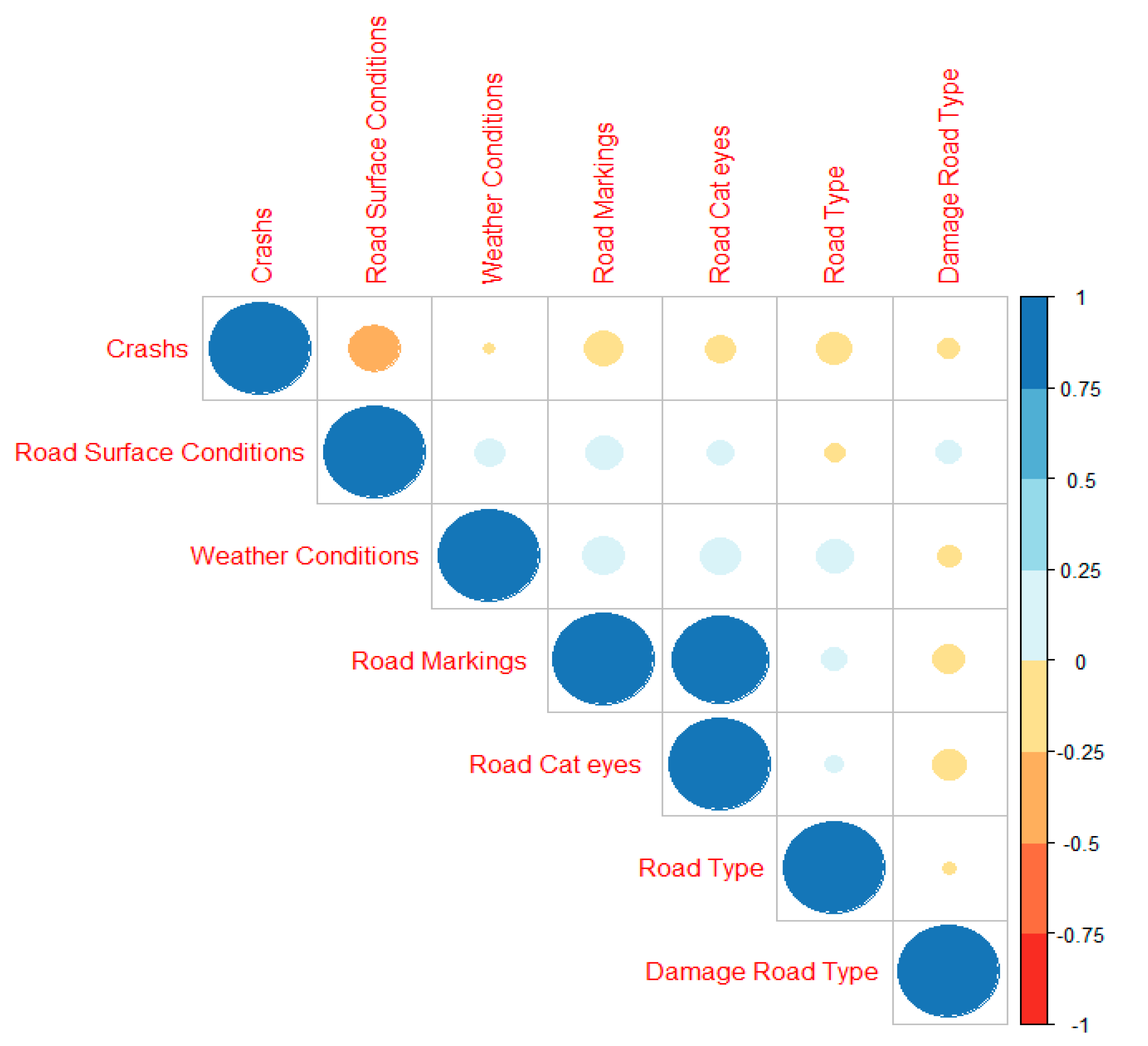
Hence, all of the values of explanatory variables were converted into indexed values. Further, the Pearson correlation among all variables is estimated, and the plot is presented in Figure 2. It is noted that all the explanatory variables have a negative relation with the number of crashes. The road surface condition is highly correlated, weather conditions are weakly correlated, and all other variables have a mild correlation with the number of crashes.

In brief, the COM–Poisson distribution is the best-fitting distribution for the crashes, and there exist some significant correlated explanatory variables. Therefore, the COM–Poisson regression is further used to measure the relationship between the crashes and the corresponding significant explanatory variables. The description of the COM–Poisson regression and the relevant control charting design structure is provided in the next section.

3. Methodology

As discussed in the previous section, the COM–Poisson distribution was identified as the best-fitting distribution for the crashes, so this section consists of the COM–Poisson regression to assess the statistically significant explanatory variables for the crashes. Further, the existing monitoring schemes based on the COM–Poisson regression and the proposed structures are also discussed in this section.

3.1. COM–Poisson Regression

Conway and Maxwell [62] proposed the Conway–Maxwell (COM)–Poisson (COM–Poisson) distribution, which is a flexible distribution to model the over/equi/under dispersed data. Let $Y$ be the random variable, then the probability mass function of the COM–Poisson distribution is defined as follows:

$$Pr\left(Y_i=y_i\right)=\frac{{\lambda }_i{}^{y_i}}{{\left(y_i!\right)}^{\nu }Z\left({\lambda }_i,\nu \right)};y=0, 1, 2, \dots ,; i=1, 2, \dots , n,$$

(2)

where ${\lambda }_i>0,$ is the rate parameter, $\nu$ is the dispersion parameter, and $Z\left({\lambda }_i,\nu \right)={\displaystyle \sum }_{j=0}^{\infty }{\lambda }_i{}^j/{\left(j!\right)}^{\nu }$ is the normalizing factor. It should be noted that, when $\nu =1$, the COM–Poisson distribution reduces to the Poisson distribution; when $\nu =0$, the COM–Poisson distribution turns into the geometric distribution; and, when $\nu =\infty$, it approaches the Bernoulli distribution. The mean and variance of the COM–Poisson distribution are expressed as follows [63]:

$$\mu =E\left(Y_i\right)=\frac{\partial log Z\left({\lambda }_i,\nu \right)}{\partial log {\lambda }_i}\approx {\lambda }_i{}^{\raisebox{1ex}{$1$}\!\left/ \!\raisebox{-1ex}{$\nu $}\right.}-\frac{\nu -1}{2\nu },$$

(3)

$${\sigma }^2=Var\left(Y_i\right)=\frac{\partial E\left(Y_i\right)}{\partial log {\lambda }_i}\approx \frac{1}{\nu }{\lambda }_i{}^{\raisebox{1ex}{$1$}\!\left/ \!\raisebox{-1ex}{$\nu $}\right.}.$$

(4)

where approximations hold for $\nu <1$or $\lambda >{10}^{\nu }$. Further, the COM-Poisson regression model is used to describe the relationship between the response variable $\left(Y\right)$ and the explanatory variables$\left(X\right)$ as a function of $\eta =X^{\prime }\beta$, where $\beta$ is the vector of unknown parameters. In this study, we are assuming link function $g$ such as $\mu =E\left(Y\right)=g^{-1}\left(\eta \right)$by following [64]. Suppose the likelihood function of the fitted model is represented by $L\left(\widehat{\mu }|Y\right)$ and for the saturated model is denoted by $L\left(Y|Y\right)$ then the overall deviance can be expressed as follows:

$$D=2\left[\log L\left(Y|Y\right)-\log L\left(\widehat{\mu }|Y\right)\right],$$

(5)

where $\widehat{\mu }=\widehat{E\left(Y\right)}$ and the deviance residuals can be obtained by the following expression:

$$\begin{gathered} d{r}_i=sign\left(y_i-{\widehat{\mu }}_i\right){\left[2\left\{y_i\nu \log \left(y_i-\frac{\nu -1}{2\nu }\right)-y_i\nu \log \left({\widehat{\mu }}_i-\frac{\nu -1}{2\nu }\right) \\ +\log \left(Z\left({\left({\widehat{\mu }}_i-\frac{\nu -1}{2\nu }\right)}^{\nu },\nu \right)\right)-\log \left(Z\left({\left(y_i-\frac{\nu -1}{2\nu }\right)}^{\nu },\nu \right)\right)\right\}\right]}^{\raisebox{1ex}{$1$}\!\left/ \!\raisebox{-1ex}{$2$}\right.}, \end{gathered}$$

(6)

where the deviance residuals are constrained such that $y_i>\mathrm{k}$ for $\nu <1/2\mathrm{k}+1, \mathrm{k}\in { \mathrm{N}}^{+}$. Moreover, the randomized quantile residuals of the COM–Poisson regression model are obtained as follows [60]:

$$q{r}_i={\mathsf{\Phi }}^{-1}\left(U_i\right),$$

(7)

where $\mathsf{\Phi }(.)$ is the cumulative distribution function of the standard normal distribution and $U_i$ is a uniform random variable between $a_i=\underset{y\to y_i}{\lim }F(y|{\widehat{\theta }}_i)$ and $b_i=\underset{y\to y_i}{\lim }F(y|{\widehat{\theta }}_i)$. It is noted that $F(.)$ is the cumulative distribution function of the response variable and ${\widehat{\theta }}_i$ is the maximum likelihood estimate of the parameter ${\theta }_i$.

3.2. Monitoring Methods Based on the COM–Poisson Regression

Control charts are a well-known methodology of the SPC tool kit because of their efficacy in temporal monitoring of the time series process. A traditional control chart has two decision lines (i.e., lower control limit (LCL) and upper control limit (UCL)) along with a centerline. A plotting point refers to an in-control (IC) state if it lies between decision lines; otherwise, the plotting point is considered as out-of-control (OOC). Control charts have been used for numerous applications across various domains [65,66,67,68,69,70,71,72,73,74].

3.2.1. Existing COM–Poisson Model-Based Control Charts

Park et al. [60] and Park et al. [61] proposed Shewhart model-based control charts to monitor the COM–Poisson process. In these studies, the authors have used deviance residuals $\left(dr\right)$ and randomized quantile residuals $\left(qr\right)$ to define the plotting statistics. In the Shewhart model-based control charts, we define the plotting quantity as $r=dr$ or $r=qr.$ This quantity $r$ of the COM–Poisson regression is used as a plotting statistic against the control limits given below:

$$\begin{gathered} LCL=E\left(r\right)-L_{S1} \sqrt{Var\left(r\right)}, \\ UCL=E\left(r\right)+L_{S2} \sqrt{Var\left(r\right)}, \end{gathered}$$

(8)

where $L_{S1}$ and $L_{S2}$ are specified to achieve the fixed in-control average run length $(AR{L}_0)$. The chart declared an OOC point when any plotting statistic falls outside of the above-defined control limits; otherwise, points are declared as IC. It is noted that, when $r=dr$, the said chart is known as the DR-COM–P Shewhart chart, while when $r=qr$, it is named as the QR-COM–P Shewhart chart.

3.2.2. Proposed COM–Poisson Model-Based Control Charts

The Shewhart charts are memory-less charts, which means they are designed based on current information [75]. Therefore, they are less prone to detect small shifts in the process. When the objective of the monitoring is to detect small to moderate shifts in the process, then EWMA and CUSUM charts are the alternatives [76]. The EWMA and CUSUM structures are also known as memory type charts as they used past information along with current information [77,78]. Hence, for the monitoring of small to moderate shifts, we have designed EWMA and CUSUM based charts in this study.

DR/QR-COM–P EWMA Control Charts

The EWMA statistic based on the residuals $r$ (i.e., $r=dr$ or $r=qr$) given in Equations (6) and (7) for the COM–Poisson regression is defined as follows:

$$Z_i=\lambda r_i+\left(1-\lambda \right)Z_{i-1}; i=1, 2, \dots , n$$

(9)

where $\mathsf{\lambda }$ is the smoothing parameter such that $0<\mathsf{\lambda }\le 1$ and the starting value of the EWMA statistic is the process target (i.e., ${\mathrm{Z}}_0=E\left(r\right)$). The limits of the EWMA charts are given as follows:

$$\begin{gathered} LCL=E\left(r\right)-L_{E1}\sqrt{\frac{\mathsf{\lambda }}{2-\mathsf{\lambda }}Var\left(r\right)}, \\ UCL=E\left(r\right)+L_{E2} \sqrt{\frac{\mathsf{\lambda }}{2-\mathsf{\lambda }}Var\left(r\right)}. \end{gathered}$$

(10)

The charting constant $L_{\mathrm{E}1}$and $L_{\mathrm{E}2}$ is set to obtain the fixed $AR{L}_0$. When $r=dr$, the chart is named as the DR-COM–P EWMA chart, while when $r=qr$, it is known as the QR-COM–P EWMA chart. The EWMA chart signals an OOC point when any plotting statistic $\left(Z_i\right)$ exceeds the control limits; otherwise, processes are declared as IC.

DR/QR-COM–P CUSUM Control Charts

The structure of the CUSUM chart is divided into two separate one-sided CUSUM statistics, i.e., $C^{+}$ and $C^{-}$, which are defined as follows:

$$C_i^{+}=max\left[0, \left(r_i-E\left(r\right)\right)-K+C_{i-1}^{+}\right],$$

(11)

$$C_i^{-}=min\left[0, \left(r_i-E\left(r\right)\right)+K+C_{i-1}^{-}\right],$$

(12)

where $K$ is the reference value, and the starting values of the afore-mentioned CUSUM statistics are taken equal to zero (i.e., $C_0^{+}=C_0^{-}=0$). The upper CUSUM statistic $C^{+}$ monitors the deviations above the target value$E\left(r\right)$, while deviations below the target value are monitored through the lower CUSUM statistic $C^{-}.$ The CUSUM chart signals an OOC residual when $C_i^{-}<-h_1\sqrt{Var\left(r\right)}$ and/or $C_i^{+}>h_2\sqrt{Var\left(r\right)}$; otherwise, residuals are considered IC. Moreover, the parameters K, $h_1$, and $h_2$ are carefully chosen against the pre-specified ${ARL}_0$ to determine the performance of the CUSUM chart. Furthermore, it is to be noted that the CUSUM chart is known as the DR-COM–P CUSUM chart when $r=dr$ and the QR-COM–P CUSUM chart when $r=qr$.

4. Simulation-Based Assessment of Proposed Charts

In this section, we will provide a simulation study and the algorithm used to determine the coefficients of control limits. Moreover, the evaluation of the proposed charts and their comparison with the existing Shewhart structures are also presented.

4.1. Simulation Settings of COM–Poisson Model

For the evaluation of the proposed EWMA and CUSUM charts and the comparative analysis with existing Shewhart charts, we have used the following data generation model:

$$y_i~COM-Poisson\left({\lambda }_i, \nu \right)$$

where ${\lambda }_i=exp\left(E\left(y_i\right)\right)=exp\left({\beta }_0+{\beta }_1{X}_{1i}+{\beta }_2{X}_{2i}\right)$, $i=1, 2, \dots n$ is the mean function and $\nu$ is the dispersion parameter. The $X_1$ and $X_2$ are independent auxiliary variables, generated through a standard normal distribution (i.e., $X_1~N\left(0, 1\right)$ and $X_2~N\left(0, 1\right)$). The parameters ${\beta }_0$ are considered equal to 0.5, ${\beta }_1=0.25,$ ${\beta }_2=-0.5,$ and the sample size is fixed as 1000 (i.e., $n=1000$). Further, for the full coverage COM–Poisson model, varying choices of dispersion parameters were considered (i.e., $\nu =0.5, 1.0, 1.5$) to assess the performance of the proposed charts.

In the COM–Poisson model, ${\lambda }_i$ and $\nu$are the fundamental parameters, where the main objective is to detect an increasing shift in ${\lambda }_i$ at the fixed dispersion parameter $\nu$. Therefore, we evaluated the performance of the control charts by considering the shifts in the${\lambda }_i,$ such that the process changes from ${\lambda }_i$ to ${\lambda }_i+\delta \sqrt{Var\left(r\right)}$. It is to be mentioned that the choices of δ and ν are made as listed below:

δ = 0(0.02)0.24 when ν = 0.5,

δ = 0(0.25)3 when ν = 1.0 or 1.5.

Previous studies have proposed different evaluation metrics to assess the predictive performance of control charts. For example, Mahmood [59] used run length (RL) properties such as average run length (ARL) and standard deviation of run length (SDRL) to evaluate the model-based charts under zero-inflated models. For the current study, we are also evaluating the proposed EWMA and CUSUM charts based on the ARL and SDRL metrics. The ARL is the average number of samples until a signal occurs, which is further categorized into in-control ARL $(AR{L}_0)$ and out-of-control ARL $(AR{L}_1)$. The charts are designed based on the fixed $AR{L}_0$ and a chart having minimum $AR{L}_1$ is declared as the best chart among all others.

4.2. Algorithm for Charting Constants

As mentioned in Section 3.2, the control limits of each chart depend on the charting constants such as $L_{S1}, L_{S2}, L_{E1}, L_{E2}, h_1,$and $h_2$. The procedure to find the control charting constants for the stated charts at pre-specified ${ARL}_0=200$ is illustrated in the following steps:

i.

Generate a data set of fixed sample size n using simulated model structure given in Section 4.1.

ii.

Fit the COM–Poisson model on the data set and obtain the deviance residuals (dr) given in (6) and randomized quantile residuals (qr) expressed in (7). Further, estimate the mean and standard error of the dr and qr.

iii.

For the Shewhart charts, set the values of L_S1 and L_S2, and fix L_E1 and L_E2 for the EWMA chart. Similarly, fix the random values h₁ and h₂ for each CUSUM chart. Further, obtain the control limit(s) and control chart statistic(s) using the estimates from step ii and selected values.

iv.

In the case of Shewhart control charts, plot the dr and qr values against their respective control limits given in (8). For the EWMA control charts, use the respective dr and qr for obtaining the respective EWMA statistics using (9) and plot it against the respective control limits given in (10). However, in the case of CUSUM control charts, use the respective dr and qr for obtaining the respective CUSUM statistics using (11) and (12), and compare these statistics with their respective decision intervals.

v.

Repeat steps i–iv for a large number of runs to obtain specified $AR{L}_0$.

If pre-specified $AR{L}_0$ is not obtained, then adjust the afore-mentioned selected values and repeat steps i–v until pre-specified $AR{L}_0$ is achieved. It is noted that residuals sometimes showed asymmetry behavior. Therefore, we have set the limits in such a way that each side of the chart shows ${ARL}_0\approx 400$ to obtain an overall ${ARL}_0=200$. Further, the control charting constants are reported in

Table 3. Control charting constants for the existing and proposed charts. EWMA, exponentially weighted moving; CUSUM, cumulative sum.

Charts	$\mathit{\lambda } \mathit{o}\mathit{r} \mathit{K}$	$\mathit{r}$	$\mathit{v}=0.5$		$\mathit{v}=1$		$\mathit{v}=1.5$
Shewhart	-		${\mathit{L}}_{\mathit{S}\mathbf{1}}$	${\mathit{L}}_{\mathit{S}\mathbf{2}}$	${\mathit{L}}_{\mathit{S}\mathbf{1}}$	${\mathit{L}}_{\mathit{S}\mathbf{2}}$	${\mathit{L}}_{\mathit{S}\mathbf{1}}$	${\mathit{L}}_{\mathit{S}\mathbf{2}}$
		$\mathit{q}\mathit{r}$	2.64	3.05	2.47	3.16	2.3	3.3
		$\mathit{d}\mathit{r}$	2.55	3.05	2.31	2.95	2.11	2.82
EWMA			${\mathit{L}}_{\mathit{E}\mathbf{1}}$	${\mathit{L}}_{\mathit{E}\mathbf{2}}$	${\mathit{L}}_{\mathit{E}\mathbf{1}}$	${\mathit{L}}_{\mathit{E}\mathbf{2}}$	${\mathit{L}}_{\mathit{E}\mathbf{1}}$	${\mathit{L}}_{\mathit{E}\mathbf{2}}$
	0.20	$\mathit{q}\mathit{r}$	2.55	2.76	2.46	2.84	2.40	2.90
		$\mathit{d}\mathit{r}$	2.51	2.77	2.48	2.77	2.5	2.69
	0.35	$\mathit{q}\mathit{r}$	2.62	2.90	2.49	3.00	2.40	3.08
		$\mathit{d}\mathit{r}$	2.55	2.89	2.51	2.85	2.46	2.76
	0.50	$\mathit{q}\mathit{r}$	2.65	2.95	2.46	3.10	2.38	3.18
		$\mathit{d}\mathit{r}$	2.58	2.95	2.46	2.9	2.37	2.785
CUSUM			${\mathit{h}}_{\mathbf{1}}$	${\mathit{h}}_{\mathbf{2}}$	${\mathit{h}}_{\mathbf{1}}$	${\mathit{h}}_{\mathbf{2}}$	${\mathit{h}}_{\mathbf{1}}$	${\mathit{h}}_{\mathbf{2}}$
	0.50	$\mathit{q}\mathit{r}$	3.60	4.15	3.10	4.10	2.80	4.10
		$\mathit{d}\mathit{r}$	3.60	4.20	3.56	4.30	4.10	4.35
	1.00	$\mathit{q}\mathit{r}$	1.75	2.30	1.40	2.31	1.14	2.30
		$\mathit{d}\mathit{r}$	1.70	2.35	1.58	2.36	1.70	2.32
	1.50	$\mathit{q}\mathit{r}$	1.05	1.41	0.67	1.46	0.43	1.47
		$\mathit{d}\mathit{r}$	1.01	1.45	0.80	1.50	0.72	1.43

at different choices of dispersion parameters.

4.3. Performance Analysis

In this section, we have presented a comparative performance evaluation of existing and proposed charts schemes using the results obtained from an extensive simulation study with ${10}^6$ iterations. The performance of memory type and memoryless control charts is assessed and reported in terms of $ARL$ and $SDRL$ in

Table 4. Average run length (ARL) profiles of the control charts at fixed v = 1.5. SDRL, standard deviation of run length.

r	δ	Shewhart		EWMA						CUSUM
		$\mathit{A}\mathit{R}\mathit{L}$	$\mathit{S}\mathit{D}\mathit{R}\mathit{L}$	λ = 0.20		λ = 0.35		λ = 0.50		K = 0.5		K = 1.0		K = 1.5
				$\mathit{A}\mathit{R}\mathit{L}$	$\mathit{S}\mathit{D}\mathit{R}\mathit{L}$	$\mathit{A}\mathit{R}\mathit{L}$	$\mathit{S}\mathit{D}\mathit{R}\mathit{L}$	$\mathit{A}\mathit{R}\mathit{L}$	$\mathit{S}\mathit{D}\mathit{R}\mathit{L}$	$\mathit{A}\mathit{R}\mathit{L}$	$\mathit{S}\mathit{D}\mathit{R}\mathit{L}$	$\mathit{A}\mathit{R}\mathit{L}$	$\mathit{S}\mathit{D}\mathit{R}\mathit{L}$	$\mathit{A}\mathit{R}\mathit{L}$	$\mathit{S}\mathit{D}\mathit{R}\mathit{L}$
$\mathit{q}\mathit{r}$	0.00	200.37	208.22	200.10	199.20	200.16	201.49	200.59	204.72	200.61	201.95	200.39	203.12	200.04	209.59
	0.25	164.88	168.03	136.64	133.88	145.41	148.26	149.79	152.07	135.33	138.85	143.97	149.62	156.99	166.40
	0.50	123.14	125.16	76.33	75.70	88.97	89.35	100.39	103.50	82.06	80.91	98.29	100.46	112.85	117.26
	0.75	93.86	98.41	45.20	41.99	55.97	55.10	64.73	64.36	48.47	45.57	66.91	67.08	81.83	84.89
	1.00	69.32	70.64	29.33	25.35	36.30	34.68	43.97	43.81	32.89	29.76	45.16	44.53	60.56	61.87
	1.25	52.60	53.82	20.91	17.61	25.57	23.71	31.21	30.92	22.36	19.34	32.49	32.09	45.56	46.75
	1.50	42.46	43.30	16.00	12.68	19.19	16.76	23.34	22.15	17.16	14.02	24.58	24.25	34.29	34.94
	1.75	33.33	34.10	12.93	9.72	15.05	13.02	18.07	16.67	13.66	10.51	18.97	17.93	26.90	26.93
	2.00	27.08	27.19	10.55	7.39	12.17	9.98	14.48	12.92	11.34	8.23	15.04	13.59	21.97	21.63
	2.25	22.12	22.24	9.09	6.05	10.17	8.07	11.92	10.46	9.55	6.69	12.62	11.39	17.33	16.89
	2.50	18.89	18.59	8.07	5.23	8.62	6.67	9.88	8.39	8.14	5.44	10.45	9.06	14.44	14.23
	2.75	15.76	15.29	7.13	4.40	7.54	5.67	8.62	7.08	7.36	4.70	8.71	7.35	12.13	11.42
	3.00	13.71	13.39	6.41	3.81	6.71	4.83	7.57	6.10	6.56	3.99	7.63	6.34	10.59	9.70
$\mathit{d}\mathit{r}$	0.00	200.88	204.85	200.19	197.14	199.85	198.61	200.49	197.93	199.31	195.60	200.30	199.94	199.71	203.73
	0.25	162.38	165.66	136.63	138.08	141.40	142.40	150.93	154.23	126.46	125.23	148.30	152.17	152.02	158.18
	0.50	125.16	131.27	71.55	69.92	83.59	83.46	92.63	94.88	67.60	62.51	94.84	96.69	105.78	111.20
	0.75	92.92	96.54	41.29	39.15	50.79	49.28	59.30	59.87	40.34	35.54	60.78	62.85	75.36	79.02
	1.00	70.40	72.37	26.21	22.21	32.11	30.02	39.25	38.03	26.82	22.81	39.79	39.37	51.53	52.69
	1.25	52.71	54.98	19.66	15.68	22.72	20.26	27.76	26.97	19.10	14.66	27.44	25.71	38.07	38.26
	1.50	41.29	42.84	14.88	11.29	17.45	14.90	20.13	18.11	14.97	10.45	20.24	18.22	28.24	28.18
	1.75	32.98	33.72	11.93	8.33	13.17	10.85	16.04	14.56	11.98	8.08	15.45	13.56	21.25	20.59
	2.00	26.73	27.45	10.04	6.52	11.26	8.92	12.72	11.10	10.27	6.61	12.95	11.34	17.26	16.40
	2.25	21.79	22.19	8.72	5.54	9.31	6.97	10.74	9.13	8.87	5.17	10.42	8.62	14.16	13.41
	2.50	18.23	17.86	7.62	4.58	8.06	5.95	9.17	7.71	7.89	4.42	8.92	7.18	11.49	10.69
	2.75	15.53	15.44	6.86	3.93	7.11	4.95	7.79	6.17	7.14	3.84	7.50	5.82	9.96	8.74
	3.00	13.38	13.10	6.24	3.41	6.29	4.14	6.79	5.18	6.48	3.32	6.57	4.86	8.62	7.76

,

Table 5. ARL profiles of the control charts at fixed v = 1.0.

r	δ	Shewhart		EWMA						CUSUM
		$\mathit{A}\mathit{R}\mathit{L}$	$\mathit{S}\mathit{D}\mathit{R}\mathit{L}$	λ = 0.20		λ = 0.35		λ = 0.50		K = 0.5		K = 1.0		K = 1.5
				$\mathit{A}\mathit{R}\mathit{L}$	$\mathit{S}\mathit{D}\mathit{R}\mathit{L}$	$\mathit{A}\mathit{R}\mathit{L}$	$\mathit{S}\mathit{D}\mathit{R}\mathit{L}$	$\mathit{A}\mathit{R}\mathit{L}$	$\mathit{S}\mathit{D}\mathit{R}\mathit{L}$	$\mathit{A}\mathit{R}\mathit{L}$	$\mathit{S}\mathit{D}\mathit{R}\mathit{L}$	$\mathit{A}\mathit{R}\mathit{L}$	$\mathit{S}\mathit{D}\mathit{R}\mathit{L}$	$\mathit{A}\mathit{R}\mathit{L}$	$\mathit{S}\mathit{D}\mathit{R}\mathit{L}$
$\mathit{q}\mathit{r}$	0.00	200.37	202.70	199.74	192.68	200.30	198.23	199.75	195.82	199.06	193.71	200.96	204.77	200.28	206.45
	0.25	129.47	132.73	80.30	79.39	94.44	94.84	107.25	110.86	85.10	83.42	110.95	112.91	124.85	129.47
	0.50	71.27	72.26	30.40	26.62	38.11	36.78	46.92	45.58	32.73	28.89	49.81	49.79	64.43	66.01
	0.75	40.92	41.25	15.88	12.38	18.93	17.07	23.17	22.03	16.94	13.73	24.82	23.77	35.91	37.05
	1.00	25.24	25.77	10.27	7.15	11.50	9.27	13.82	12.25	10.72	7.64	14.61	13.07	20.42	19.78
	1.25	16.56	16.51	7.40	4.56	7.98	6.02	9.14	7.66	7.64	4.81	9.59	8.10	13.27	12.73
	1.50	11.31	11.07	5.83	3.34	5.97	4.10	6.57	5.10	6.10	3.53	6.87	5.37	8.85	8.09
	1.75	8.38	7.95	4.85	2.55	4.82	3.06	5.12	3.72	4.95	2.59	5.30	3.99	6.47	5.60
	2.00	6.35	5.84	4.13	2.02	3.99	2.35	4.17	2.85	4.25	2.12	4.18	2.92	4.97	4.17
	2.25	4.94	4.48	3.64	1.67	3.45	1.92	3.49	2.22	3.71	1.75	3.52	2.31	4.08	3.19
	2.50	4.05	3.60	3.29	1.45	3.05	1.62	3.04	1.85	3.28	1.43	3.06	1.87	3.37	2.59
	2.75	3.32	2.78	2.98	1.27	2.71	1.34	2.71	1.54	3.00	1.26	2.66	1.60	2.86	2.05
	3.00	2.88	2.34	2.74	1.11	2.50	1.21	2.45	1.31	2.79	1.15	2.39	1.34	2.50	1.73
$\mathit{d}\mathit{r}$	0.00	200.23	202.96	199.38	194.64	199.76	193.14	200.89	198.64	199.80	203.56	200.91	222.24	200.41	208.51
	0.25	136.80	145.64	83.14	81.57	94.13	98.60	106.98	110.46	79.19	79.00	102.87	110.19	125.53	133.74
	0.50	77.34	82.27	29.73	25.96	36.21	33.69	43.76	45.56	30.48	26.82	45.66	46.41	62.97	66.09
	0.75	44.07	47.46	15.74	12.24	18.14	15.85	21.86	20.95	15.88	12.14	22.52	20.96	32.02	31.26
	1.00	27.20	28.66	10.31	7.06	11.14	8.83	13.02	11.60	10.27	6.77	13.30	11.72	18.64	17.80
	1.25	17.06	17.38	7.41	4.40	7.77	5.58	8.72	7.25	7.77	4.64	8.61	6.93	11.83	10.97
	1.50	11.97	11.75	5.85	3.14	5.82	3.90	6.38	4.88	6.03	3.18	6.34	4.89	8.12	7.34
	1.75	8.59	8.53	4.86	2.41	4.70	2.91	4.99	3.69	5.07	2.40	4.92	3.38	5.98	4.97
	2.00	6.45	6.21	4.26	1.99	3.96	2.29	4.04	2.67	4.38	1.96	4.04	2.56	4.79	3.81
	2.25	5.12	4.80	3.70	1.64	3.43	1.81	3.44	2.11	3.87	1.66	3.37	1.99	3.74	2.88
	2.50	4.09	3.67	3.35	1.43	3.08	1.54	2.98	1.78	3.51	1.42	2.99	1.69	3.19	2.34
	2.75	3.44	2.96	3.04	1.20	2.71	1.28	2.68	1.51	3.17	1.22	2.67	1.43	2.74	1.84
	3.00	2.90	2.37	2.83	1.09	2.47	1.12	2.40	1.30	2.90	1.06	2.42	1.28	2.45	1.59

and

Table 6. ARL profiles of the control charts at fixed v = 0.5.

r	δ	Shewhart		EWMA						CUSUM
		$\mathit{A}\mathit{R}\mathit{L}$	$\mathit{S}\mathit{D}\mathit{R}\mathit{L}$	λ = 0.20		λ = 0.35		λ = 0.50		K = 0.5		K = 1.0		K = 1.5
				$\mathit{A}\mathit{R}\mathit{L}$	$\mathit{S}\mathit{D}\mathit{R}\mathit{L}$	$\mathit{A}\mathit{R}\mathit{L}$	$\mathit{S}\mathit{D}\mathit{R}\mathit{L}$	$\mathit{A}\mathit{R}\mathit{L}$	$\mathit{S}\mathit{D}\mathit{R}\mathit{L}$	$\mathit{A}\mathit{R}\mathit{L}$	$\mathit{S}\mathit{D}\mathit{R}\mathit{L}$	$\mathit{A}\mathit{R}\mathit{L}$	$\mathit{S}\mathit{D}\mathit{R}\mathit{L}$	$\mathit{A}\mathit{R}\mathit{L}$	$\mathit{S}\mathit{D}\mathit{R}\mathit{L}$
$\mathit{q}\mathit{r}$	0.00	199.92	197.68	199.77	197.66	199.66	197.60	199.01	199.83	200.6336	200.29	200.52	204.99	200.81	205.67
	0.02	191.75	193.69	168.23	163.88	178.58	176.14	180.64	181.08	175.31	172.24	190.31	188.88	190.07	192.50
	0.04	165.33	164.83	119.52	119.42	133.58	134.57	136.60	141.13	128.09	128.18	153.55	159.81	162.17	163.69
	0.06	139.96	142.41	76.81	73.28	93.61	94.71	98.39	101.56	85.05	84.27	114.21	119.52	120.35	123.58
	0.08	105.22	107.26	51.82	49.35	63.52	61.48	72.97	74.87	56.35	53.85	83.61	86.99	93.47	94.07
	0.10	82.39	83.68	36.02	32.36	43.04	41.34	51.00	50.92	40.49	37.67	59.16	59.62	68.21	69.17
	0.12	61.08	62.49	26.38	22.64	31.19	28.95	35.95	35.09	28.53	25.34	42.57	43.50	49.29	48.62
	0.14	45.26	45.23	20.42	16.84	23.76	21.59	27.18	26.45	22.04	18.38	30.58	29.37	37.29	37.37
	0.16	35.17	35.96	15.87	12.37	18.66	16.63	20.97	19.85	17.20	13.64	23.78	22.46	28.56	28.39
	0.18	27.59	27.39	13.08	9.85	14.88	13.08	16.83	15.48	13.84	10.69	17.98	16.52	22.34	21.71
	0.20	21.48	20.90	11.00	7.87	12.47	10.50	13.03	11.56	11.67	8.61	14.67	13.74	17.45	16.89
	0.22	17.99	17.60	9.43	6.49	10.24	8.33	11.32	10.05	9.89	6.79	11.75	10.43	14.61	13.91
	0.24	14.62	14.76	8.34	5.60	8.67	6.74	9.32	8.10	8.75	5.93	9.97	8.57	11.64	10.87
$\mathit{d}\mathit{r}$	0.00	200.52	199.30	200.19	199.84	199.33	194.99	200.41	200.74	199.66	192.00	199.61	199.02	200.27	193.29
	0.02	196.57	195.34	171.49	171.71	172.49	170.55	180.34	180.76	166.03	165.71	177.50	180.43	184.85	185.98
	0.04	171.59	169.98	118.44	119.15	131.21	130.89	136.55	138.78	120.65	119.94	143.96	146.51	145.95	147.57
	0.06	138.66	143.86	75.82	73.45	88.19	88.80	98.77	100.04	78.89	74.64	105.05	110.33	114.76	118.17
	0.08	105.73	108.79	51.11	47.32	60.45	59.59	68.33	68.65	54.04	50.59	74.95	75.04	84.43	88.14
	0.10	80.32	83.41	35.55	32.33	41.91	40.11	49.96	51.31	38.34	35.23	52.17	53.79	60.18	60.84
	0.12	60.21	62.05	26.07	22.55	30.37	28.69	35.52	34.84	27.07	23.14	37.78	37.72	45.78	44.86
	0.14	45.83	46.91	20.38	17.14	22.96	20.68	26.45	25.44	20.96	17.81	28.32	27.31	33.62	33.33
	0.16	35.92	36.16	16.09	12.90	17.85	15.40	20.28	19.00	16.24	12.36	21.26	20.62	26.04	25.75
	0.18	27.44	27.57	13.08	10.07	14.34	12.24	16.58	15.77	13.64	10.18	16.94	15.91	20.38	19.89
	0.20	21.67	21.13	10.97	8.23	11.87	9.65	13.08	11.92	11.29	8.03	13.86	12.84	15.91	15.19
	0.22	17.57	17.11	9.45	6.70	10.09	8.01	11.10	9.58	9.89	6.86	11.20	9.85	13.26	12.63
	0.24	14.71	14.29	8.47	5.80	8.56	6.93	9.37	7.95	8.72	5.85	9.53	8.12	11.27	10.77

. In addition, the impact of the reference value $\left(K\right)$ on the performance of the CUSUM control charts is investigated. Similarly, the impact of the smoothing parameter (λ) on the performance of the EWMA control charts is also evaluated. Figure 3 shows the impact of charting parameters on the performance of the proposed charts.

4.3.1. Analysis Based on Under-Dispersed Data

By assuming $\nu =1.5,$ the detection ability of the proposed EWMA and CUSUM charts is compared with the existing Shewhart charts in Table 4. The findings depict that the charts based on deviance residuals (i.e., DR-COM–P Shewhart, DR-COM–P EWMA, and DR-COM–P CUSUM) are relatively more efficient to detect increasing shifts in the mean. For example, when $\delta =2$, the $ARL$ of the DR-COM–P Shewhart chart is reported as 26.73, which is lower than the $ARL$ value of 27.08 of the QR-COM–P Shewhart chart. Further, at fixed $\lambda =0.2,$ a shift $\delta =1$ may cause 85 and 87 percent reduction in the $ARL$ of the QR-COM–P EWMA and DR-COM–P EWMA charts, respectively. Similarly, at fixed $K=0.5,$ a 192.47-unit and 191.42-unit decrease is noted in the $ARL$ of QR-COM–P CUSUM and DR-COM–P CUSUM charts, respectively, due to a shift $\delta =2.5$.

It is also noted that the EWMA type charts (i.e., QR-COM–P EWMA and DR-COM–P EWMA) have relatively better detection ability compared with CUSUM and Shewhart type charts. For example, at fixed $\lambda =0.2$and $K=0.5,$when $\delta =1$, the $ARL$ of QR-COM–P Shewhart is reported as 69.32, while $ARL$ values of 29.33 and 32.98 are noted for the QR-COM–P EWMA and QR-COM–P CUSUM charts, respectively. Similarly, a shift $\delta =1.5$ may cause 79, 93, and 92 percent reduction in the $ARL$ of DR-COM–P Shewhart, DR-COM–P EWMA, and DR-COM–P CUSUM charts, respectively.

4.3.2. Analysis Based on Equi-Dispersed Data

The findings of the comparative analysis between the proposed and existing charts at fixed $\nu =1$ are given in Table 5. The results showed that the QR-COM–P Shewhart and DR-COM–P Shewhart charts depicted almost similar performance. Moreover, the deviance residuals-based charts (i.e., DR-COM–P EWMA and DR-COM–P CUSUM) have better detection ability as compared with quantile residual-based charts (i.e., QR-COM–P EWMA and QR-COM–P CUSUM). For example, at fixed $\lambda =0.35,$ when $\delta =0.5$, the $ARL$ of the DR-COM–P EWMA chart is reported as 36.21, which is lower than the $ARL$ value of 38.11 of the QR-COM–P EWMA chart. Further, at fixed $K=1,$ a shift $\delta =1.75$ may cause 97 and 98 percent reduction in the $ARL$ of QR-COM–P CUSUM and DR-COM–P CUSUM charts, respectively.

Similar to the findings of under-dispersed data, the EWMA type charts (i.e., QR-COM–P EWMA and DR-COM–P EWMA) under equi-dispersed data showed relatively better performance compared with Shewhart and CUSUM type charts. For example, at fixed $\lambda =0.35$and $K=1,$a shift $\delta =1.25$ may cause 92, 96, and 95 percent reduction in the $ARL$ of QR-COM-P Shewhart, QR-COM–P EWMA, and QR-COM–P CUSUM charts, respectively. Similarly, when $\delta =1.75$, the $ARL$ of DR-COM–P Shewhart is reported as 8.59, while $ARL$ values of 4.70 and 4.92 are noted for the DR-COM–P EWMA and DR-COM–P CUSUM charts, respectively.

4.3.3. Analysis Based on Over-Dispersed Data

By fixing $\nu =0.5,$the performance of the proposed EWMA and CUSUM charts is compared with the that of Shewhart charts in Table 6. Once again, it is noted that the charts based on deviance residuals (i.e., DR-COM–P Shewhart, DR-COM–P EWMA, and DR-COM–P CUSUM) have relatively better detection ability as compared with the quantile residual-based charts (i.e., QR-COM–P Shewhart, QR-COM–P EWMA, and QR-COM–P CUSUM). For example, when $\delta =0.12$, the $ARL$ of the DR-COM–P Shewhart chart is reported as 60.21, which is lower than the $ARL$ value of 61.08 of the QR-COM–P Shewhart chart. Further, at fixed $\lambda =0.5,$ a shift $\delta =0.08$ may cause 63 and 66 percent reduction in the $ARL$ of QR-COM–P EWMA and DR-COM–P EWMA charts, respectively. Similarly, at fixed $K=1.5,$ a 186.21-unit and 187.01-unit decrease is noted in the $ARL$ of the QR-COM–P CUSUM and DR-COM–P CUSUM charts due to a shift $\delta =0.22$.

Similar to the other findings, under over-dispersion data, the EWMA type charts (i.e., QR-COM–P EWMA and DR-COM–P EWMA) have relatively better detection ability as compared with Shewhart and CUSUM type charts. For example, at fixed $\lambda =0.5$and $K=1.5,$when $\delta =0.10,$ the $ARL$ of QR-COM–P Shewhart is reported as 82.39, while $ARL$ values of 51.00 and 68.21 are noted for the QR-COM–P EWMA and QR-COM–P CUSUM charts, respectively. Similarly, a shift $\delta =0.20$ may cause 89, 93, and 92 percent reduction in the $ARL$ of DR-COM–P Shewhart, DR-COM–P EWMA, and DR-COM–P CUSUM charts, respectively.

4.4. Impact of Charting Parameters $\lambda$ and $K$

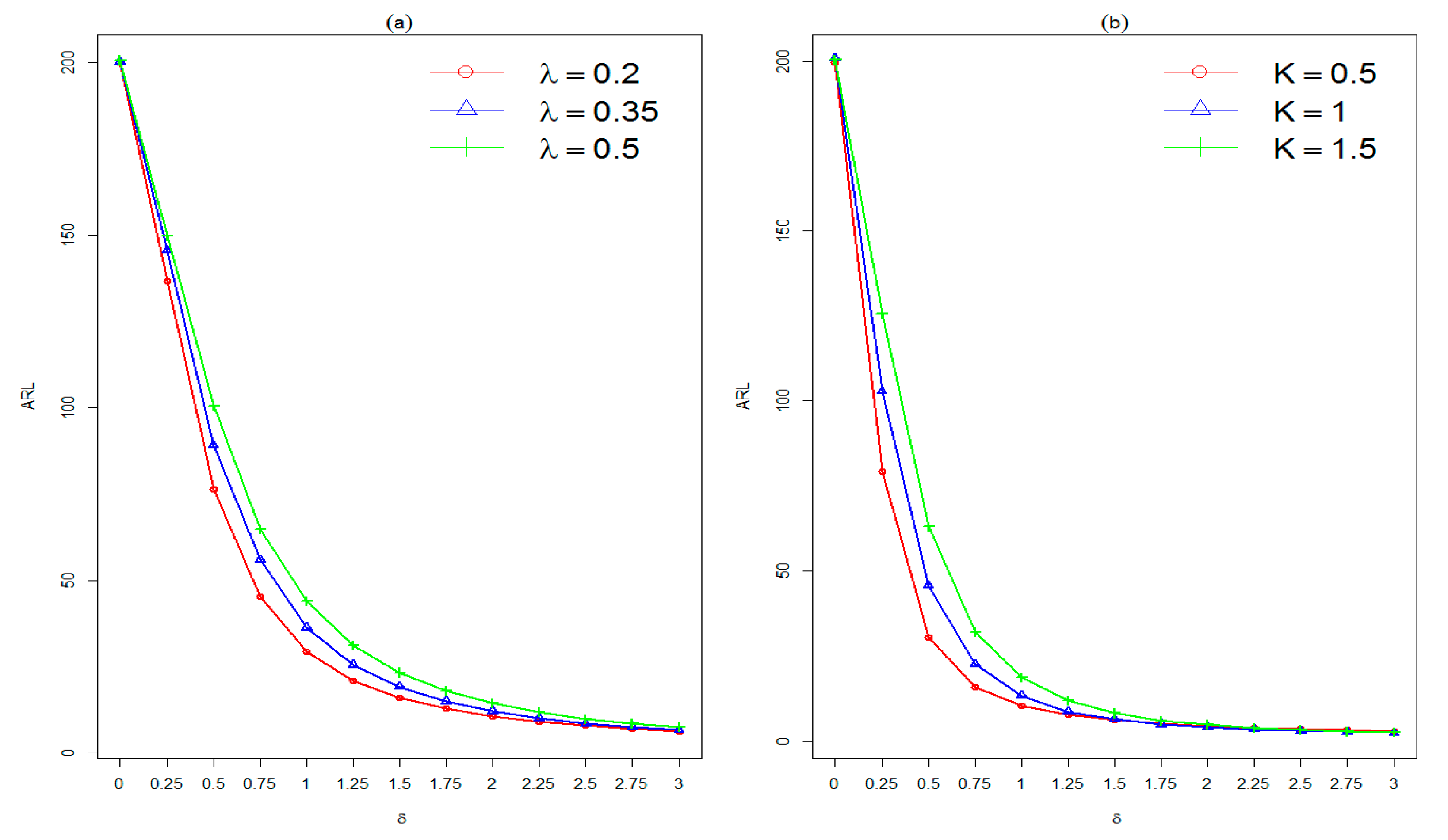
The smoothing parameter $\lambda$ plays a vital role in the detection ability of the EWMA chart. Therefore, for brevity, the performance of the QR-COM–P EWMA chart for three choices of $\lambda$ (i.e., $\lambda =0.20, 0.35$, and $0.50)$ at fixed $v=1.5$ is plotted in Figure 3a. It is clearly seen that the detection ability of the QR-COM–P EWMA chart increases with the decrease of $\lambda$. For example, when $\delta =1.5$, the $ARL$ values of QR-COM–P EWMA are reported as 16.00, 19.19, and 23.34 against $\lambda =0.20, 0.35,$ and $0.50$, respectively.

In the CUSUM chart, the reference value $K$ is used to set the detection ability of the CUSUM chart. To notice the effect of $K$, we have drawn the results of the DR-COM–P CUSUM chart for three choices of $K$ (i.e., $K=0.5, 1.0,$ and $1.5)$ at fixed $v=1$. The $ARL$ curves revealed an inverse relationship between the detection ability of the CUSUM chart and reference value $K$. For example, when $\delta =0.25,$ the $ARL$ values of the DR-COM–P CUSUM chart are reported as 79.19, 102.87, and 125.53 against $K=0.5, 1.0,$ and $1.5$, respectively. The impact of charting parameters λ and K is shown above in Figure 3.

5. Implementation of Proposed Methods for Real-Time Crash Monitoring

In this section, we have applied the COM–Poisson regression to observe the significant factors contributing to the crash occurrences. Further, based on the estimated model, we have implemented the proposed charts for real-time monitoring.

A close view of Figure 1 shows that daily crash counts witness a steady downward trend after December 2018 and do not exceed this point again. This downward trend in observed crash record may be attributed to the implementation and enforcement of a new automated citation system introduced at the start of 2018 under the SAHER program [79]. SAHER is an automated system adopted for controlling traffic using a digital network of cameras connected to the central information center. Hence, crash data to this point act as IC data and are used for establishing control chart structure, and the remaining data are considered for the monitoring phase (in an OOC state).

As discussed in Section 2, the indexed values of road type, road surface conditions, damage type post-crash, weather conditions, road markings, and cat eyes are considered as possible explanatory variables for the crashes. Therefore, to assess the most significant explanatory variables, we have computed pairwise COM–Poisson regression models based on IC data. Out of 63 different models, the following model is considered as the best model based on the minimum values of $AIC=6164.0668$, $BIC=6182.9137$, and $Log-liklihood=-3078.0334$.

$$Crashes=exp\left(1.7891-0.0670 \mathrm{IVRT}-0.0475 \mathrm{IVRSC}\right)$$

(13)

where IVRT and IVRSC represent the indexed values of road type and road surface conditions, respectively. It is evident from the results of the IC model that the intercept term, road type, and road surface conditions are statistically significant explanatory/predictor variables for the crashes with p-values < 0.01 and standard errors of $0.1052, 0.0266,$ and 0.0120, respectively. Moreover, it is also observed that the estimated dispersion parameter is observed as $\widehat{\nu }=0.4169,$ which is also statistically significant with a p-value of less than 0.01 and a standard error of $0.021$.

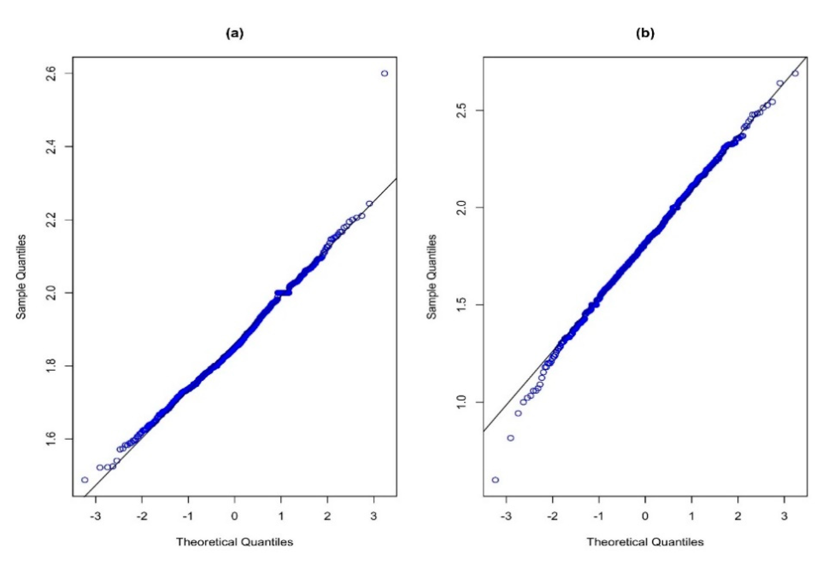
For the development of the control chart setup, we have considered the above-mentioned IC model. Further, using the normal probability plots plotted in Figure 4, it is observed that the IVRT is a normally distributed variable with a mean of 1.86 and variance of 0.017 (cf. Figure 4a). Similarly, the road surface conditions also follow a normal distribution, having a mean of 1.81 and variance of 0.08 (cf. Figure 4b). Hence, based on these estimates and following Section 4.1, we have set up the simulation settings of the COM–Poisson model, and control charting constants are obtained using the algorithm given in Section 4.1, and are reported in

Table 7. Control charting constants of the charts based on the in-control (IC) model of crashes data.

$\mathit{r}$	Shewhart		EWMA		CUSUM
	${\mathit{L}}_{\mathit{S}\mathbf{1}}$	${\mathit{L}}_{\mathit{S}\mathbf{2}}$	${\mathit{L}}_{\mathit{E}\mathbf{1}}$	${\mathit{L}}_{\mathit{E}\mathbf{2}}$	${\mathit{h}}_{\mathbf{1}}$	${\mathit{h}}_{\mathbf{2}}$
$\mathit{q}\mathit{r}$	2.80	2.81	2.80	2.78	0.96	0.965
$\mathit{d}\mathit{r}$	2.69	2.75	3.20	3.18	0.956	0.96

. It is noted that we have assumed ${ARL}_0=200$, $\lambda =0.50$, and $K=1.5$.

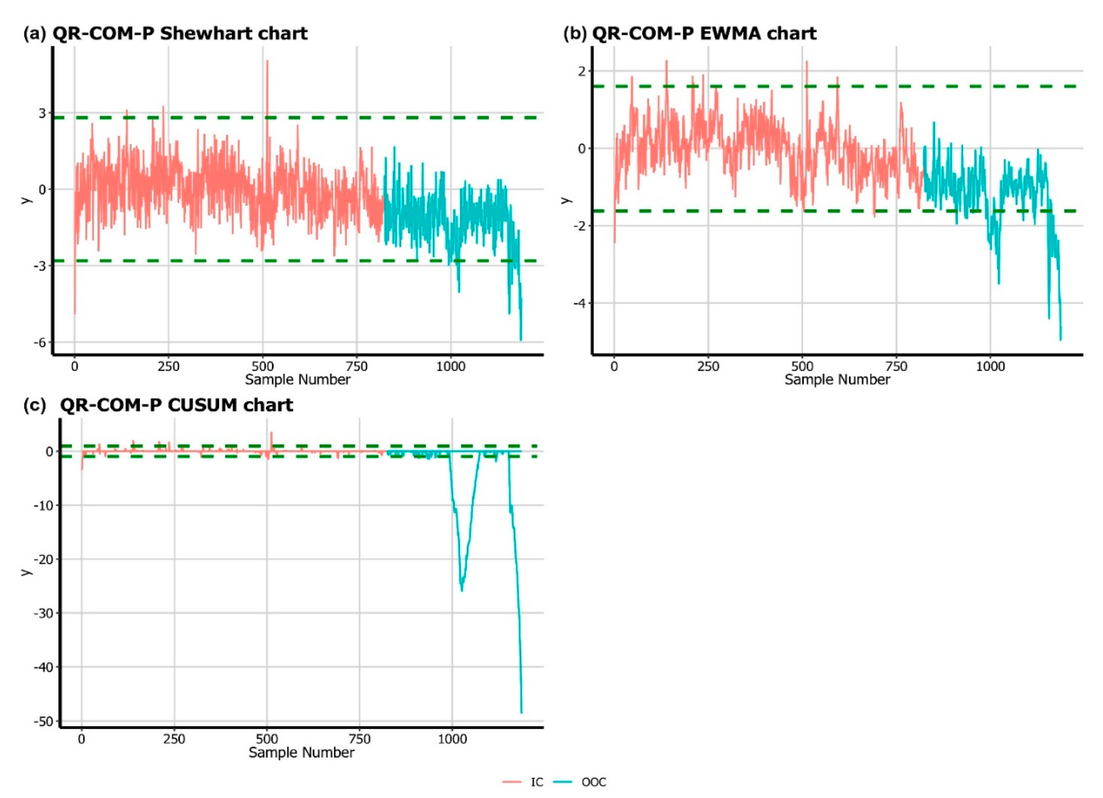
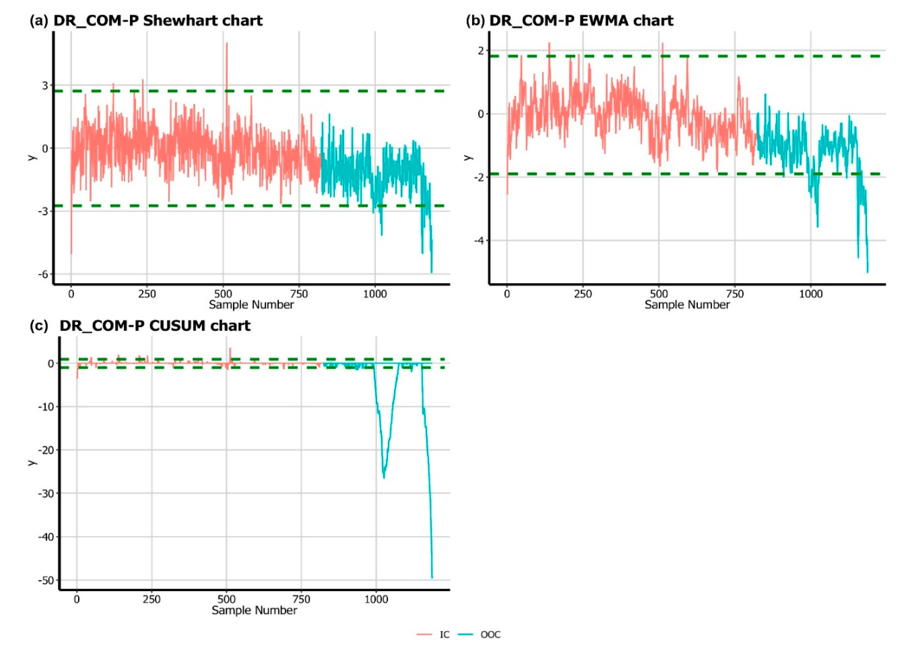
The randomized quantile residual-based charts (i.e., QR-COM–P Shewhart, QR-COM–P EWMA, and QR-COM–P CUSUM) and deviance residuals-based charts (i.e., DR-COM–P Shewhart, DR-COM–P EWMA, and DR-COM–P CUSUM) are implemented on the crash data set. The QR-COM–P Shewhart, QR-COM–P EWMA, and QR-COM–P CUSUM charts are plotted in Figure 5, whereas the DR-COM–P Shewhart, DR-COM–P EWMA, and DR-COM–P CUSUM are given in Figure 6. In every chart, the red line represents plotting statistics based on the residuals from IC model, while the blue line is used to show plotting statistics based on OOC residuals. Further, green dotted lines are used to show the control limits of every chart.

It is observed from Figure 5 and Figure 6 that the QR-COM–P Shewhart chart signaled four false alarms with 26 OOC points, while the same number of signals is detected by the DR-COM–P Shewhart chart. The QR-COM–P EWMA and DR-COM–P EWMA charts show 13 and 14 false alarms, while 76 and 80 OOC signals are reported by QR-COM–P EWMA and DR-COM–P EWMA charts, respectively. Further, 22 and 23 false alarms are reported by the QR-COM–P CUSUM and DR-COM–P CUSUM charts, respectively, while 124 and 126 OOC points are signaled by the QR-COM–P CUSUM and DR-COM–P CUSUM charts, respectively.

6. Summary, Conclusions, and Recommendations

During the past few decades, many studies have proposed a wide range of statistical modeling approaches to explore the relationships between causal factors and crash occurrence. However, very few have focused on developing germane procedures for real-time highway safety surveillance using available crash records. Control charts are useful tools in SPC with numerous applications for active event monitoring. Traditionally, the Poisson distribution is frequently used to interpret the data for a control chart; however, it may be inappropriate to model under-dispersed or over-dispersed data. This study proposes the EWMA and CUSUM control chart scheme for highway safety monitoring using three years of crash data (2017–2019) for rural highways in Saudi Arabia. During the first stage of the study, three well-known count data distribution models (Poisson, negative binomial, and COM–Poisson) were investigated to identify the most appropriate distribution model for the data. The findings showed that the COM–Poisson regression model is the best fitted statistical model.

During the second stage of the study, EWMA and CUSUM type charts based on the residuals (i.e., deviance or randomized quantile residuals) of the COM–Poisson regression model were developed from a crash monitoring perspective. An extensive simulation study was designed to assess the performance evaluation of the proposed control charts scheme and their comparison with the existing Shewhart type chart. The results revealed that the charts based on deviance residuals (i.e., DR-COM–P Shewhart, DR-COM–P EWMA, and DR-COM–P CUSUM) were relatively more flexible and efficient in detecting increasing shifts in the mean. Further, it was noted the EWMA type charts (i.e., QR-COM–P EWMA and DR-COM–P EWMA) outperformed Shewhart and CUSUM type charts in terms of considered evaluation metrics (both ARL and SDRL). The results from the simulation study also indicated an inverse relationship of the reference value ($K)$smoothing parameter $\lambda$ with the performance of the GLM-based CUSUM EWMA control charts. Finally, during the third stage of the study, the proposed monitoring methods were successfully implemented on real-time crash data. The findings of this study could provide useful essential guidance to policy- and decision-makers for initiating concrete steps to improve users’ road safety. The proposed real-time monitoring for highway safety surveillance can guide on effective and proactive implementation of different hazard control measures to mitigate the occurrence of future traffic crashes. Some of the quick hazard control measures suggested in this regard include measures such as improving the surface conditions, installation of variable message signs for guidance and warnings, raised pavements, delineators on horizontal curves, weather warning systems, ramp metering, and induction of speed and traffic calming measures at crash hotpots, among others.

This study has a few limitations that might be addressed in future studies. It is worth noting that the present study was designed assuming the known parameters. It will be interesting to see the effect of parameter estimation on the charts in forthcoming studies. The performance of the proposed control chart scheme was verified using limited (three years) real-life crash data. Further investigations using other detailed datasets are needed for a more precise assessment of the statistical properties of the suggested monitoring procedures. Future studies could also consider the application of the proposed methods for real-life monitoring of crashes by individual severity groups (fatal, injury, and property damage) or specific crash types. The monitoring scheme based on crash severity classes will be helpful in prioritizing prevention strategies with the emphasis placed on more severe crashes. Future studies could also investigate the impact of auto-correlated response variables. Furthermore, one may adopt advanced charting structures such as moving average, progressive moving average, mixed EWMA–CUSUM, and HEWMA type charts.

References

- Global Status Report on Road Safety 2018; World Health Organization: Geneva, Switzerland, 2019.
- Yu, R.; Wang, Y.; Quddus, M.; Li, J. A Marginalized Random Effects Hurdle Negative Binomial Model for Analyzing Refined-Scale Crash Frequency Data. Anal. Methods Accid. Res. 2019, 22, 100092. [Google Scholar] [CrossRef]
- Global Status Report on Road Safety 2015; World Health Organization: Geneva, Switzerland, 2015.
- Jamal, A.; Rahman, M.T.; Al-Ahmadi, H.M.; Ullah, I.M.; Zahid, M. Intelligent Intersection Control for Delay Optimization: Using Meta-Heuristic Search Algorithms. Sustainability 2020, 12, 1896. [Google Scholar] [CrossRef] [Green Version]
- Al-Turki, M.; Jamal, A.; Al-Ahmadi, H.M.; Al-Sughaiyer, M.A.; Zahid, M. On the Potential Impacts of Smart Traffic Control for Delay, Fuel Energy Consumption, and Emissions: An NSGA-II-Based Optimization Case Study from Dhahran, Saudi Arabia. Sustainability 2020, 12, 7394. [Google Scholar] [CrossRef]
- Mohamed, H.A. Estimation of Socio-Economic Cost of Road Accidents in Saudi Arabia: Willingness-To-Pay Approach (WTP). Adv. Manag. Appl. Econ. 2015, 5, 43. [Google Scholar]
- Jamal, A.; Umer, W. Exploring the Injury Severity Risk Factors in Fatal Crashes with Neural Network. IJERPH 2020, 17, 7466. [Google Scholar] [CrossRef]
- Kaaf, K.A.; Abdel-Aty, M. Transferability and Calibration of Highway Safety Manual Performance Functions and Development of New Models for Urban Four-Lane Divided Roads in Riyadh, Saudi Arabia. Transp. Res. Rec. 2015, 2515, 70–77. [Google Scholar] [CrossRef]
- Islam, M.; Alharthi, M.; Alam, M. The Impacts of Climate Change on Road Traffic Accidents in Saudi Arabia. Climate 2019, 7, 103. [Google Scholar] [CrossRef] [Green Version]
- Alarifi, S.A.; Alkahtani, K.F.; Abdel-Aty, M.A.; Kher, S.O.; Mohammed, A.M.; AlMojil, A.H. Corridor Safety Evaluation in a Developing Country Using a Survey Based Approach. J. Transp. Saf. Secur. 2019, 11, 189–206. [Google Scholar] [CrossRef]
- Shanks, N.J.; Ansari, M.; Ai-Kalai, D. Road Traffic Accidents in Saudi Arabia. Public Health 1994, 108, 27–34. [Google Scholar] [CrossRef]
- Touahmia, M. Identification of Risk Factors Influencing Road Traffic Accidents. Eng. Technol. Appl. Sci. Res. 2018, 8, 2417–2421. [Google Scholar] [CrossRef]
- Al-Tit, A.A.; Ben Dhaou, I.; Albejaidi, F.M.; Alshitawi, M.S. Traffic Safety Factors in the Qassim Region of Saudi Arabia. Sage Open 2020, 10. [Google Scholar] [CrossRef]
- Jamal, A.; Rahman, M.T.; Al-Ahmadi, H.M.; Mansoor, U. The Dilemma of Road Safety in the Eastern Province of Saudi Arabia: Consequences and Prevention Strategies. Int. J. Environ. Res. Public Health 2020, 17, 157. [Google Scholar] [CrossRef] [Green Version]
- AlKheder, S.; Al-Rashidi, M. Bayesian Hierarchical Statistics for Traffic Safety Modelling and Forecasting. Int. J. Inj. Control Saf. Promot. 2020, 27, 99–111. [Google Scholar] [CrossRef] [PubMed]
- Mohamed, S.A.; Mohamed, K.; Al-Harthi, H.A. Investigating Factors Affecting the Occurrence and Severity of Rear-End Crashes. Transp. Res. Procedia 2017, 25, 2098–2107. [Google Scholar] [CrossRef]
- Farag, S.G.; Hashim, I.H. Safety Performance Appraisal at Roundabouts: Case Study of Salalah City in Oman. J. Transp. Saf. Secur. 2017, 9, 67–82. [Google Scholar] [CrossRef]
- Cafiso, S.; Di Graziano, A.; Di Silvestro, G.; La Cava, G.; Persaud, B. Development of Comprehensive Accident Models for Two-Lane Rural Highways Using Exposure, Geometry, Consistency and Context Variables. Accid. Anal. Prev. 2010, 42, 1072–1079. [Google Scholar] [CrossRef] [PubMed]
- Hou, Q.; Tarko, A.P.; Meng, X. Investigating Factors of Crash Frequency with Random Effects and Random Parameters Models: New Insights from Chinese Freeway Study. Accid. Anal. Prev. 2018, 120, 1–12. [Google Scholar] [CrossRef]
- Haghighi, N.; Liu, X.C.; Zhang, G.; Porter, R.J. Impact of Roadway Geometric Features on Crash Severity on Rural Two-Lane Highways. Accid. Anal. Prev. 2018, 111, 34–42. [Google Scholar] [CrossRef]
- Xing, F.; Huang, H.; Zhan, Z.; Zhai, X.; Ou, C.; Sze, N.N.; Hon, K.K. Hourly Associations between Weather Factors and Traffic Crashes: Non-Linear and Lag Effects. Anal. Methods Accid. Res. 2019, 24, 100109. [Google Scholar] [CrossRef]
- Lord, D.; Mannering, F. The Statistical Analysis of Crash-Frequency Data: A Review and Assessment of Methodological Alternatives. Transp. Res. Part A Policy Pract. 2010, 44, 291–305. [Google Scholar] [CrossRef] [Green Version]
- Aguero-Valverde, J.; Jovanis, P.P. Analysis of Road Crash Frequency with Spatial Models. Transp. Res. Rec. 2008, 2061, 55–63. [Google Scholar] [CrossRef]
- Pappalardo, G.; Cafiso, S.; Di Graziano, A.; Severino, A. Decision Tree Method to Analyze the Performance of Lane Support Systems. Sustainability 2021, 13, 846. [Google Scholar] [CrossRef]
- Afghari, A.P.; Washington, S.; Haque, M.M.; Li, Z. A Comprehensive Joint Econometric Model of Motor Vehicle Crashes Arising from Multiple Sources of Risk. Anal. Methods Accid. Res. 2018, 18, 1–14. [Google Scholar] [CrossRef]
- Afghari, A.P.; Haque, M.M.; Washington, S.; Smyth, T. Effects of Globally Obtained Informative Priors on Bayesian Safety Performance Functions Developed for Australian Crash Data. Accid. Anal. Prev. 2019, 129, 55–65. [Google Scholar] [CrossRef] [PubMed]
- Valen, A.; Bogstrand, S.T.; Vindenes, V.; Frost, J.; Larsson, M.; Holtan, A.; Gjerde, H. Driver-Related Risk Factors of Fatal Road Traffic Crashes Associated with Alcohol or Drug Impairment. Accid. Anal. Prev. 2019, 131, 191–199. [Google Scholar] [CrossRef]
- Lord, D.; Manar, A.; Vizioli, A. Modeling Crash-Flow-Density and Crash-Flow-V/C Ratio Relationships for Rural and Urban Freeway Segments. Accid. Anal. Prev. 2005, 37, 185–199. [Google Scholar] [CrossRef] [PubMed]
- Kim, S.; Ulfarsson, G.F. Traffic Safety in an Aging Society: Analysis of Older Pedestrian Crashes. J. Transp. Saf. Secur. 2019, 11, 323–332. [Google Scholar] [CrossRef]
- McGwin, G., Jr.; Brown, D.B. Characteristics of Traffic Crashes among Young, Middle-Aged, and Older Drivers. Accid. Anal. Prev. 1999, 31, 181–198. [Google Scholar] [CrossRef]
- Tauhidur Rahman, M.; Jamal, A.; Al-Ahmadi, H.M. Examining Hotspots of Traffic Collisions and Their Spatial Relationships with Land Use: A GIS-Based GeographicallyWeighted Regression Approach for Dammam, Saudi Arabia. ISPRS Int. J. Geo-Inf. 2020, 9, 540. [Google Scholar] [CrossRef]
- Hong, J.; Tamakloe, R.; Park, D. A Comprehensive Analysis of Multi-Vehicle Crashes on Expressways: A Double Hurdle Approach. Sustainability 2019, 11, 2782. [Google Scholar] [CrossRef] [Green Version]
- Zahid, M.; Chen, Y.; Khan, S.; Jamal, A.; Ijaz, M.; Ahmed, T. Predicting Risky and Aggressive Driving Behavior among Taxi Drivers: Do Spatio-Temporal Attributes Matter? Int. J. Environ. Res. Public Health 2020, 17, 3937. [Google Scholar] [CrossRef]
- Ullah, I.; Jamal, A.; Subhan, F. Public Perception of Autonomous Car: A Case Study for Pakistan. Adv. Transp. Stud. 2019, 49, 145–154. [Google Scholar]
- Afghari, A.P.; Haque, M.M.; Washington, S. Applying Fractional Split Model to Examine the Effects of Roadway Geometric and Traffic Characteristics on Speeding Behavior. Traffic Inj. Prev. 2018, 19, 860–866. [Google Scholar] [CrossRef] [Green Version]
- Zahid, M.; Chen, Y.; Jamal, A.; Al-Ahmadi, H.M.; Al-Ofi, A.K. Adopting Machine Learning and Spatial Analysis Techniques for Driver Risk Assessment: Insights from a Case Study. Int. J. Environ. Res. Public Health 2020, 17, 5193. [Google Scholar] [CrossRef]
- Ma, X.; Chen, F.; Chen, S. Modeling Crash Rates for a Mountainous Highway by Using Refined-Scale Panel Data. Transp. Res. Rec. 2015, 2515, 10–16. [Google Scholar] [CrossRef]
- Yu, R.; Xiong, Y.; Abdel-Aty, M. A Correlated Random Parameter Approach to Investigate the Effects of Weather Conditions on Crash Risk for a Mountainous Freeway. Transp. Res. Part C Emerg. Technol. 2015, 50, 68–77. [Google Scholar] [CrossRef]
- Ahmed, M.M.; Abdel-Aty, M.; Yu, R. Assessment of Interaction of Crash Occurrence, Mountainous Freeway Geometry, Real-Time Weather, and Traffic Data. Transp. Res. Rec. 2012, 2280, 51–59. [Google Scholar] [CrossRef] [Green Version]
- Hammad, H.M.; Ashraf, M.; Abbas, F.; Bakhat, H.F.; Qaisrani, S.A.; Mubeen, M.; Fahad, S.; Awais, M. Environmental Factors Affecting the Frequency of Road Traffic Accidents: A Case Study of Sub-Urban Area of Pakistan. Environ. Sci. Pollut. Res. 2019, 26, 11674–11685. [Google Scholar] [CrossRef] [PubMed]
- Qiu, L.; Nixon, W.A. Effects of Adverse Weather on Traffic Crashes: Systematic Review and Meta-Analysis. Transp. Res. Rec. 2008, 2055, 139–146. [Google Scholar] [CrossRef]
- Lee, J.; Nam, B.; Abdel-Aty, M. Effects of Pavement Surface Conditions on Traffic Crash Severity. J. Transp. Eng. 2015, 141, 04015020. [Google Scholar] [CrossRef]
- National Highway Traffic Safety Administration. A Compilation of Motor Vehicle Crash Data from the Fatality Analysis Reporting System and the General Estimates System; United States Department of Transportation: Washington, DC, USA, 2014.
- Shaon, M.R.R.; Qin, X.; Shirazi, M.; Lord, D.; Geedipally, S.R. Developing a Random Parameters Negative Binomial-Lindley Model to Analyze Highly over-Dispersed Crash Count Data. Anal. Methods Accid. Res. 2018, 18, 33–44. [Google Scholar] [CrossRef]
- Guikema, S.D.; Goffelt, J.P. A Flexible Count Data Regression Model for Risk Analysis. Risk Anal. Int. J. 2008, 28, 213–223. [Google Scholar] [CrossRef]
- Chen, J.-H. A Double Generally Weighted Moving Average Chart for Monitoring the COM-Poisson Processes. Symmetry 2020, 12, 1014. [Google Scholar] [CrossRef]
- Lord, D.; Guikema, S.D.; Geedipally, S.R. Application of the Conway–Maxwell–Poisson Generalized Linear Model for Analyzing Motor Vehicle Crashes. Accid. Anal. Prev. 2008, 40, 1123–1134. [Google Scholar] [CrossRef]
- Lord, D.; Geedipally, S.R.; Guikema, S.D. Extension of the Application of Conway-Maxwell-Poisson Models: Analyzing Traffic Crash Data Exhibiting Underdispersion. Risk Anal. Int. J. 2010, 30, 1268–1276. [Google Scholar] [CrossRef] [PubMed] [Green Version]
- Schuh, A.; Camelio, J.A.; Woodall, W.H. Control Charts for Accident Frequency: A Motivation for Real-Time Occupational Safety Monitoring. Int. J. Inj. Control Saf. Promot. 2014, 21, 154–162. [Google Scholar] [CrossRef]
- Skinner, K.R.; Montgomery, D.C.; Runger, G.C. Generalized Linear Model-Based Control Charts for Discrete Semiconductor Process Data. Qual. Reliab. Eng. Int. 2004, 20, 777–786. [Google Scholar] [CrossRef]
- Asgari, A.; Amiri, A.; Niaki, S.T.A. A New Link Function in GLM-Based Control Charts to Improve Monitoring of Two-Stage Processes with Poisson Response. Int. J. Adv. Manuf. Technol. 2014, 72, 1243–1256. [Google Scholar] [CrossRef]
- Jearkpaporn, D.; Borror, C.M.; Runger, G.C.; Montgomery, D.C. Process Monitoring for Mean Shifts for Multiple Stage Processes. Int. J. Prod. Res. 2007, 45, 5547–5570. [Google Scholar] [CrossRef]
- Amiri, A.; Yeh, A.B.; Asgari, A. Monitoring Two-Stage Processes with Binomial Data Using Generalized Linear Model-Based Control Charts. Qual. Technol. Quant. Manag. 2016, 13, 241–262. [Google Scholar] [CrossRef]
- Shang, Y.; Tsung, F.; Zou, C. Profile Monitoring with Binary Data and Random Predictors. J. Qual. Technol. 2011, 43, 196–208. [Google Scholar] [CrossRef]
- Urbieta, P.; Lee HO, L.; Alencar, A. CUSUM and EWMA Control Charts for Negative Binomial Distribution. Qual. Reliab. Eng. Int. 2017, 33, 793–801. [Google Scholar] [CrossRef]
- Alencar, A.P.; Lee HO, L.; Albarracin, O.Y.E. CUSUM Control Charts to Monitor Series of Negative Binomial Count Data. Stat. Methods Med. Res. 2017, 26, 1925–1935. [Google Scholar] [CrossRef]
- Kinat, S.; Amin, M.; Mahmood, T. GLM-Based Control Charts for the Inverse Gaussian Distributed Response Variable. Qual. Reliab. Eng. Int. 2020, 36, 765–783. [Google Scholar] [CrossRef]
- Amin, M.; Mahmood, T.; Kinat, S. Memory Type Control Charts with Inverse-Gaussian Response: An Application to Yarn Manufacturing Industry. Trans. Inst. Meas. Control 2020, 0142331220952965. [Google Scholar] [CrossRef]
- Mahmood, T.; Xie, M. Models and Monitoring of Zero-Inflated Processes: The Past and Current Trends. Qual. Reliab. Eng. Int. 2019, 35, 2540–2557. [Google Scholar] [CrossRef]
- Park, K.; Jung, D.; Kim, J. Control Charts Based on Randomized Quantile Residuals. Appl. Stoch. Models Bus. Ind. 2020, 36, 716–729. [Google Scholar] [CrossRef]
- Park, K.; Kim, J.-M.; Jung, D. GLM-Based Statistical Control-Charts for Dispersed Count Data with Multicollinearity between Input Variables. Qual. Reliab. Eng. Int. 2018, 34, 1103–1109. [Google Scholar] [CrossRef]
- Conway, R.W.; Maxwell, W.L. A Queuing Model with State Dependent Service Rates. J. Ind. Eng. 1962, 12, 132–136. [Google Scholar]
- Shmueli, G.; Minka, T.P.; Kadane, J.B.; Borle, S.; Boatwright, P. A Useful Distribution for Fitting Discrete Data: Revival of the Conway–Maxwell–Poisson Distribution. J. R. Stat. Soc. Ser. C (Appl. Stat.) 2005, 54, 127–142. [Google Scholar] [CrossRef]
- Sellers, K.F.; Shmueli, G. A Flexible Regression Model for Count Data. Ann. Appl. Stat. 2010, 4, 943–961. [Google Scholar] [CrossRef] [Green Version]
- Riaz, M.; Abbas, N.; Mahmood, T. A Communicative Property with Its Industrial Applications. Qual. Reliab. Eng. Int. 2017, 33, 2761–2763. [Google Scholar] [CrossRef]
- Mahmood, T.; Wittenberg, P.; Zwetsloot, I.M.; Wang, H.; Tsui, K.L. Monitoring Data Quality for Telehealth Systems in the Presence of Missing Data. Int. J. Med. Inform. 2019, 126, 156–163. [Google Scholar] [CrossRef] [Green Version]
- Mahmood, T. Generalized Linear Model Based Monitoring Methods for High-Yield Processes. Qual. Reliab. Eng. Int. 2020, 36, 1570–1591. [Google Scholar] [CrossRef]
- Ali, A.; Mahmood, T.; Nazir, H.Z.; Sana, I.; Akhtar, N.; Qamar, S.; Iqbal, M. Control Charts for Process Dispersion Parameter under Contaminated Normal Environments. Qual. Reliab. Eng. Int. 2016, 32, 2481–2490. [Google Scholar] [CrossRef]
- Abbas, N.; Riaz, M.; Mahmood, T. An Improved S 2 Control Chart for Cost and Efficiency Optimization. IEEE Access 2017, 5, 19486–19493. [Google Scholar] [CrossRef]
- Raji, I.A.; Lee, M.H.; Riaz, M.; Abujiya, M.R.; Abbas, N. Outliers Detection Models in Shewhart Control Charts; an Application in Photolithography: A Semiconductor Manufacturing Industry. Mathematics 2020, 8, 857. [Google Scholar] [CrossRef]
- Riaz, M.; Abbasi, S.A.; Abid, M.; Hamzat, K.A. A New HWMA Dispersion Control Chart with an Application to Wind Farm Data. Mathematics 2020, 8, 2136. [Google Scholar] [CrossRef]
- Kim, J.-M.; Wang, N.; Liu, Y.; Park, K. Residual Control Chart for Binary Response with Multicollinearity Covariates by Neural Network Model. Symmetry 2020, 12, 381. [Google Scholar] [CrossRef] [Green Version]
- Aslam, M.; Rao, G.S.; Khan, N.; Al-Abbasi, F.A. EWMA Control Chart Using Repetitive Sampling for Monitoring Blood Glucose Levels in Type-II Diabetes Patients. Symmetry 2019, 11, 57. [Google Scholar] [CrossRef] [Green Version]
- Omar, M.; Arafat, S.; Hossain, M.P.; Riaz, M. Inverse Maxwell Distribution and Statistical Process Control: An Efficient Approach for Monitoring Positively Skewed Process. Symmetry 2021, 13, 189. [Google Scholar] [CrossRef]
- Hussain, S.; Mei, S.; Riaz, M.; Abbasi, S.A. On Phase-I Monitoring of Process Location Parameter with Auxiliary Information-Based Median Control Charts. Mathematics 2020, 8, 706. [Google Scholar] [CrossRef]
- Chen, J.-H.; Lu, S.-L. A New Sum of Squares Exponentially Weighted Moving Average Control Chart Using Auxiliary Information. Symmetry 2020, 12, 1888. [Google Scholar] [CrossRef]
- Ali, S.; Abbas, Z.; Nazir, H.Z.; Riaz, M.; Zhang, X.; Li, Y. On Designing Non-Parametric EWMA Sign Chart under Ranked Set Sampling Scheme with Application to Industrial Process. Mathematics 2020, 8, 1497. [Google Scholar] [CrossRef]
- Abbas, N.; Abujiya, M.R.; Riaz, M.; Mahmood, T. Cumulative Sum Chart Modeled under the Presence of Outliers. Mathematics 2020, 8, 269. [Google Scholar] [CrossRef] [Green Version]
- Alghnam, S.; Towhari, J.; Alkelya, M.; Binahmad, A.; Bell, T.M. The Effectiveness of Introducing Detection Cameras on Compliance with Mobile Phone and Seatbelt Laws: A before-after Study among Drivers in Riyadh, Saudi Arabia. Inj. Epidemiol. 2018, 5, 1–8. [Google Scholar] [CrossRef] [Green Version]
Figure 1.
Temporal variations of observed crashes during the study period.
Figure 2.
Matrix of correlation among the explanatory variables.
Figure 3.
Impact of charting parameters: (a) impact of the smoothing parameter on the performance of the QR-Conway–Maxwell–Poisson (COM–P) exponentially weighted moving (EWMA) chart at fixed v = 1.5 and (b) effect of the reference value on the performance of the DR-COM–P cumulative sum (CUSUM) control chart at fixed v = 1. ARL, average run length.
Figure 4.
The normal probability plots: (a) for the indexed value of road type and (b) for the indexed value of road surface conditions.
Figure 5.
Implementation of randomized quantile residual-based charts on crash data. IC, in-control; OOC, out-of-control.
Figure 6.
Implementation of deviance residual-based charts on crash data.