On the Development of Triple Homogeneously Weighted Moving Average Control Chart

Abstract

To detect sustainable changes in the manufacturing processes, memory-type charting schemes are frequently functioning. The recently designed, homogenously weighted moving average (HWMA) technique is effective for identifying substantial changes in the processes. To make the HWMA chart more effective for persistent shifts in the industrial processes, a double HWMA (DHWMA) chart has been proposed recently. This study intends to develop a triple HWMA (THWMA) chart for efficient monitoring of the process mean under zero- and steady-state scenarios. The non-normal effects of monitoring characteristics under in-control situations for heavy-tailed highly skewed and contaminated normal environments are computed under both states. The relative efficiency of the proposed structure is compared with HWMA, DHWMA, exponentially weighted moving average (EWMA), double EWMA, and the more effective triple EWMA control charting schemes. The relative analysis reveals that the proposed THWMA design performs more efficiently than the existing counterparts. An illustrative application related to substrate manufacturing is also incorporated to demonstrate the proposal.

1. Introduction

In manufacturing and production industries, variations are an integral part of running processes. Control charts are statistical processes monitoring (SPM) techniques used for tracing and eliminating sudden changes in the process target to produce high yield products. Shewhart introduced the idea of the monitoring process through control charting in 1920. Quality practitioners noticed that Shewhart structure-based monitoring schemes only perform effectively in identifying large shifts in the process parameters. To understand sustainable shifts in the process, Page [1] developed a cumulative sum (CUSUM) chart that accumulates deviation from the process target. After the development of the CUSUM scheme, Roberts [2] designed an exponentially weighted moving average (EWMA) charting scheme, which has earned a lot of popularity in SPM literature and continuously growing (cf. Montgomery [3]). The EWMA charting statistic assigns more weight to the most recent information and less weight to old information, and these weights decrease exponentially among the sample information. Recently, Abbas [4] studied the homogeneously weighted moving average (HWMA) charting technique by allocating a certain weight to the freshest process value and the remaining weight homogeneously allocated among the mean of all the rest values in the working process. The relative effectiveness of the HWMA chart was found relatively better than CUSUM and EWMA charts.

Quality practitioners always require a charting structure that promptly traces small changes in the process parameters. In the SPM paradigm’s literature, many advancements and modifications on control charts exist that are continuously growing to fulfill the practitioner’s requirement of quickly shift detection. To increase the effectiveness of the Shewhart design, Lucas [5] developed a combined Shewhart–CUSUM (CS–CUSUM) chart, and Lucas and Saccucci [6] studied the CS–EWMA chart to trace shifts in the process location. Lucas and Saccucci [6] observed the steady-state behavior of the EWMA chart for monitoring the mean of the quality characteristic of interest. Runger and Montgomery [7] investigated the steady-state effect on the Shewhart control chart focusing on the process mean. Shamma and Shamma [8] suggested a double EWMA (DEWMA) scheme, and Abbas et al. [9] designed a mixed EWMA–CUSUM scheme respectively to trace small shifts in the process mean effectively. Zaman et al. [10] investigated a mixed CUSUM–EWMA chart and Abbas et al. [11] designed double progressive mean charts for the process mean shifts. Abbas et al. [12] developed an exponentially weighted moving average chart taking progressive mean (PM) as input variable and named as mixed EWMA–PM and Riaz et al. [13] studied another chart by name mixed PM–EWMA schemes respectively for efficient monitoring of the process mean. For swift tracing small noises in the mean of the process, Abid et al. [14] introduced a double HWMA (DHWMA) chart, and Raza et al. [15] designed a nonparametric HWMA chart under simple and ranked set sampling schemes for monitoring persistent shifts in the process target. Aslam et al. [16] investigated a hybrid EWMA scheme to monitor process variability. Chen and Lu [17] designed the sum of squares EWMA model using auxiliary characteristics. Recently, Alevizakos et al. [18] designed triple EWMA (TEWMA) charting methods for effectively addressing shifts in the mean of the process. The relative comparison of the charting schemes is made based on average run length (ARL), which is the average number of plotted samples before a chart produces an out-of-control (OOC) signal. $AR{L}_0$ is customry used for in-control (IC) ARL and $AR{L}_1$ for OOC ARL.

The current study intends to develop a triple HWMA (THWMA) chart, taking inspiration from Alevizakos et al. [18] for swift screening small shifts in the process. The run-length (RL) characteristics of the proposed THWMA chart are evaluated using zero and steady-state processes. The robust behavior of the proposed THWMA design is observed using heavy-tailed $t_{\left(v\right)}$ and logistic processes; for skewed nature processes, gamma distribution and an outlier in the processes contaminated normal (CN) distribution are also incorporated in this study. Expert researchers usually choose CN distribution for the assessment of design structures in the presence of outliers.

The remaining article is outlined as follows: An overview of some existing memory-type charts and proposed design is presented in Section 2. Sensitivity analysis of the proposed THWMA scheme and a relative comparison of the proposed THWMA and existing competitors are presented in Section 3. Section 4 presents real-life data application of the proposed THWMA and existing counterpart charts. Concluding remarks with some future lines are highlighted in Section 5, and the article ends with Appendix A, Appendix B, Appendix C and Appendix D showing some derivations.

2. Design Structure of the HWMA and the Proposed Triple HWMA Schemes

The design structure of HWMA, DHWMA, and the proposed THWMA schemes are presented in this section. The sensitivity analyses of the proposed design under a normal and non-normal environment are also provided in this section.

2.1. Design of HWMA Scheme

Suppose the quality characteristic $Y_{tj}$; $t=1, 2,3,\dots$ and $j=1, 2, 3,\dots ,n$ is taken from the normal distribution with known mean $\mu$ and standard deviation $\sigma$. The HWMA charting statistic proposed by Abbas [4] is written as

$$H_t=\lambda {\overline{Y}}_t+\left(1-\lambda \right){\stackrel{\overline{¯}}{Y}}_{t-1}.$$

(1)

In (1) ${\overline{Y}}_t=\frac{{{\displaystyle \sum }}_{j=1}^n{Y}_{tj}}{n},$ ${\stackrel{\overline{¯}}{Y}}_{t-1}=\frac{{\overline{Y}}_1+{\overline{Y}}_2+{\overline{Y}}_3+\dots +{\overline{Y}}_{t-1}}{t-1}$ and $\lambda \in (0,1]$ is the smoothing parameter of the HWMA statistic. The HWMA scheme performs sensitively for small shifts at small choices of $\lambda$. The mean of HWMA scheme is, $E\left(H_t\right)=\mu$ and variance of HWMA is, $var\left(H_t\right)=\frac{{\sigma }^2}{n}\left[{\lambda }^2 +\frac{{\left(1-\lambda \right)}^2}{\left(t-1\right)}\right]$ (cf. Appendix A.1, Appendix A.2, Appendix B.1 and Appendix B.2). The control limits of the HWMA chart are

$$\begin{array}{ccc}LC{L}_t& =& \{\begin{array}{cc}\mu -K\sqrt{\frac{{\sigma }^2}{n}{\lambda }^2, }\hfill & t=1\hfill \\ \mu -K\sqrt{\frac{{\sigma }^2}{n}\left[{\lambda }^2+\frac{{\left(1-\lambda \right)}^2}{\left(t-1\right)}\right],}\hfill & t>1\hfill \end{array}\\ CL& =& \mu ,\\ UC{L}_t& =& \{\begin{array}{cc}\mu +K\sqrt{\frac{{\sigma }^2}{n}{\lambda }^2, }\hfill & t=1\hfill \\ \mu +K\sqrt{\frac{{\sigma }^2}{n}\left[{\lambda }^2+\frac{{\left(1-\lambda \right)}^2}{\left(t-1\right)}\right],}\hfill & t>1\hfill \end{array}\end{array}\}$$

(2)

The HWMA scheme has two design parameters $\lambda$ and $K$, which are chosen to attain desired values of $AR{L}_0$. $K$ is known as signaling coefficient and $\lambda \in (0,1]$ is smoothing constant. The HWMA chart traces shift in the ongoing process if the statistic provided in (1) plots outside the control limits presented in (2).

2.2. Design of DHWMA Scheme

After the development of the HWMA model, Abid et al. [14] designed a double HWMA (DHWMA) chart, which proved more efficient than the HWMA method. The DHWMA charting scheme utilizes sample information twice. The DHWMA charting statistic is derived as

$$D{H}_t=\lambda H_t+\left(1-\lambda \right){\stackrel{\overline{¯}}{Y}}_{t-1}.$$

(3)

Taking $H_t=\lambda {\overline{Y}}_t+\left(1-\lambda \right){\stackrel{\overline{¯}}{Y}}_{t-1}$ from (1) and putting in (3), the DHWMA statistic more precisely becomes

$$\begin{gathered} D{H}_t=\lambda \left(\lambda {\overline{Y}}_t+\left(1-\lambda \right){\stackrel{\overline{¯}}{Y}}_{t-1}\right)+\left(1-\lambda \right){\stackrel{\overline{¯}}{Y}}_{t-1}, \\ ={\lambda }^2{\overline{Y}}_t+\lambda \left(1-\lambda \right){\stackrel{\overline{¯}}{Y}}_{t-1}+\left(1-\lambda \right){\stackrel{\overline{¯}}{Y}}_{t-1}, \\ D{H}_t={\lambda }^2{\overline{Y}}_t+\left(1-{\lambda }^2\right){\stackrel{\overline{¯}}{Y}}_{t-1}. \end{gathered}$$

(4)

In (4), ${\lambda }^2$ presents the weight allocated to the most recent measurement in the working process. The mean of DHWMA chart is, $E$$(D{H}_t)=\mu$, and its variance is, $var\left(D{H}_t\right)=\frac{{\sigma }^2}{n}\left[{\lambda }^4+\frac{{\left(1-{\lambda }^2\right)}^2}{\left(t-1\right)}\right]$ (cf. Appendix C.1 and Appendix C.2). The charting limits of the DHWMA scheme become

$$\begin{array}{ccc}LC{L}_t& =& \{\begin{array}{cc}\mu -K\sqrt{\frac{{\sigma }^2}{n}{\lambda }^4, }\hfill & t=1\hfill \\ \mu -K\sqrt{\frac{{\sigma }^2}{n}\left[{\lambda }^4+\frac{{\left(1-{\lambda }^2\right)}^2}{\left(t-1\right)}\right],}\hfill & t>1\hfill \end{array}\\ CL& =& \mu ,\\ UC{L}_t& =& \{\begin{array}{cc}\mu +K\sqrt{\frac{{\sigma }^2}{n}{\lambda }^4, }\hfill & t=1\hfill \\ \mu +K\sqrt{\frac{{\sigma }^2}{n}\left[{\lambda }^4+\frac{{\left(1-{\lambda }^2\right)}^2}{\left(t-1\right)}\right],}\hfill & t>1\hfill \end{array}\end{array}\}.$$

(5)

The design parameters of the DHWMA scheme are $\lambda$ and $K$, which are already defined in the previous section. The DHWMA statistic presented in (4) detects OOC position if it goes beyond the control limits provided in (5); otherwise, it is considered in a stable situation.

2.3. Design of the Proposed THWMA Scheme

This section intends to develop high sensitive triple HWMA (THWMA) design to identify small and sustainable changes in the process effectively. The proposed THWMA plan utilizes sample information thrice, which makes the structure efficient. Suppose the quality characteristic of interest $Y_{tj}$ has ${\overline{Y}}_1,$ ${\overline{Y}}_2$, ${\overline{Y}}_3,$ …, ${\overline{Y}}_t$,… sequence of identically and independently distribution mean of observations corresponding to each sample number. Then, the mathematical form of the proposed THWMA charting scheme is

$$T{H}_t=\lambda D{H}_t+\left(1-\lambda \right){\stackrel{\overline{¯}}{Y}}_{t-1}.$$

(6)

Putting value of $D{H}_t={\lambda }^2{\overline{Y}}_t+\left(1-{\lambda }^2\right){\stackrel{\overline{¯}}{Y}}_{t-1}$ from (4) in (6), we obtain

$$\begin{gathered} T{H}_t=\lambda \left({\lambda }^2{\overline{Y}}_t+\left(1-{\lambda }^2\right){\stackrel{\overline{¯}}{Y}}_{t-1}\right)+\left(1-\lambda \right){\stackrel{\overline{¯}}{Y}}_{t-1}, \\ ={\lambda }^3{\overline{Y}}_t+\lambda \left(1-{\lambda }^2\right){\stackrel{\overline{¯}}{Y}}_{t-1}+\left(1-\lambda \right){\stackrel{\overline{¯}}{Y}}_{t-1}, \\ T{H}_t={\lambda }^3{\overline{Y}}_t+\left(1-{\lambda }^3\right){\stackrel{\overline{¯}}{Y}}_{t-1}. \end{gathered}$$

(7)

where the $T{H}_1,$ $T{H}_2,$ $T{H}_3,$..., $T{H}_t$,… is the sequence of the proposed THWMA plotting statistic corresponding to each sample number. The mean and variance of the proposed THWMA statistic provided in (7) are $E\left(T{H}_t\right)=\mu$ and $var\left(T{H}_t\right)=\frac{{\sigma }^2}{n}\left[{\lambda }^6+\frac{{\left(1-{\lambda }^3\right)}^2}{\left(t-1\right)}\right]$ respectively (cf. Appendix D.1 and Appendix D.2). For the proposed structure, $E\left({\stackrel{\overline{¯}}{Y}}_0\right)=\mu .$ The control limits of the proposed scheme using these mean and variance become

$$\begin{array}{ccc}LC{L}_t& =& \{\begin{array}{cc}\mu -K\sqrt{\frac{{\sigma }^2}{n}{\lambda }^6, }\hfill & t=1\hfill \\ \mu -K\sqrt{\frac{{\sigma }^2}{n}\left[{\lambda }^6+\frac{{\left(1-{\lambda }^3\right)}^2}{\left(t-1\right)}\right],}\hfill & t>1\hfill \end{array}\\ CL& =& \mu ,\\ UC{L}_t& =& \{\begin{array}{cc}\mu +K\sqrt{\frac{{\sigma }^2}{n}{\lambda }^6, }\hfill & t=1\hfill \\ \mu +K\sqrt{\frac{{\sigma }^2}{n}\left[{\lambda }^6+\frac{{\left(1-{\lambda }^3\right)}^2}{\left(t-1\right)}\right],}\hfill & t>1\hfill \end{array}\end{array}\}$$

(8)

where $\lambda$ $(0<\lambda \le 1)$ shows the smoothing parameter and $K$ denotes the signaling coefficient of the proposed THWMA chart. The THWMA schemes trace the shift in the process mean if it goes above the $UC{L}_t$ or below the $LC{L}_t$ in any sample, as provided in (8). The proposed THWMA chart declines to Shewhart’s [19] chart at $\lambda =1$.

3. Evaluation of Proposed THWMA Chart

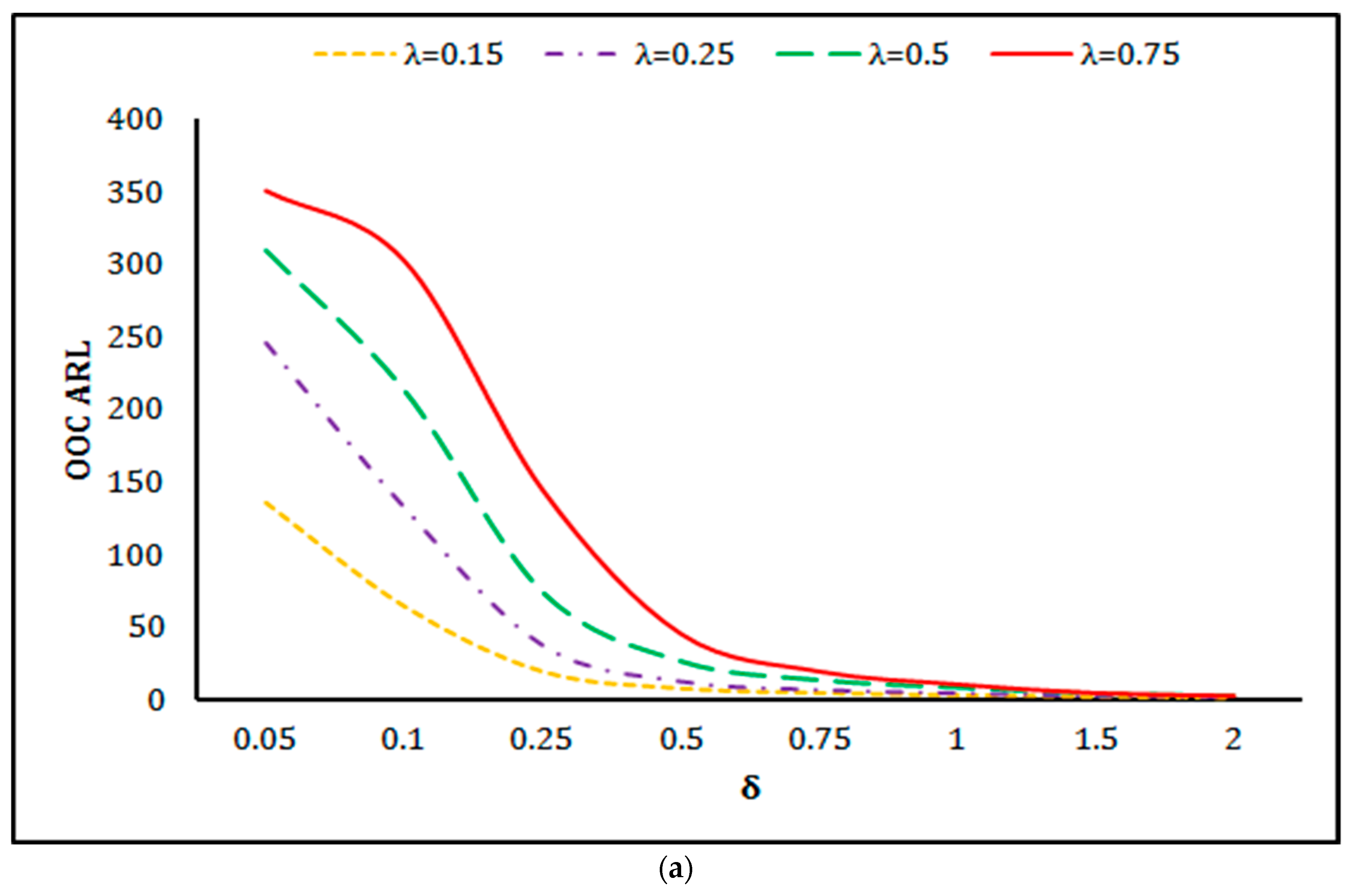
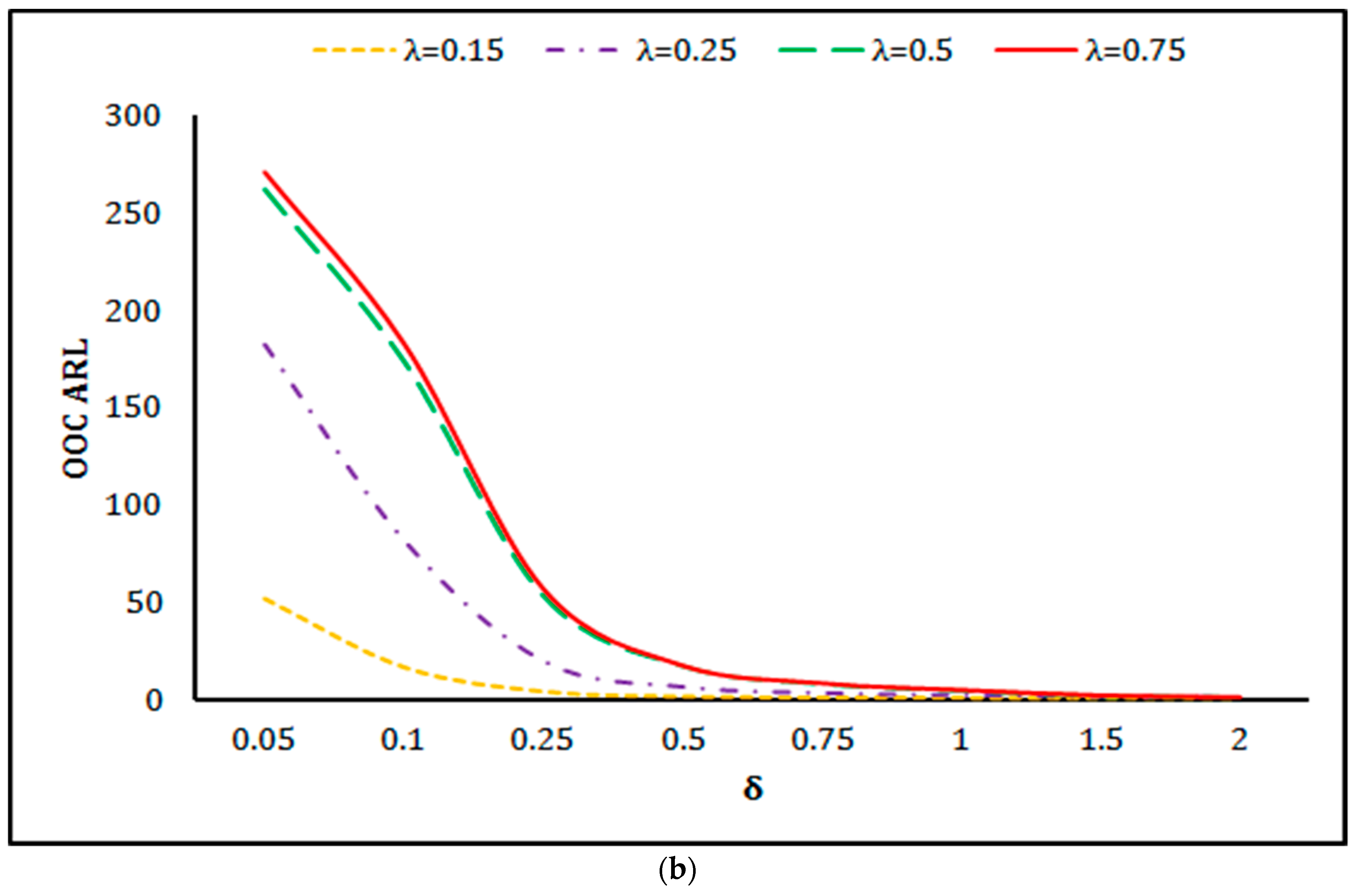
To observe the properties of the proposed THWMA chart, run length (RL) characteristics are computed in this section. The RL properties of the THWMA scheme are computed using the Monte Carlo simulation method with the codes designed in the R programming language. To evaluate the more reliable results of RL profiles, $1\times {10}^5$ iterations are carried out, following Abbasi [20] and Hussain et al. [21] because the proposed THWMA structure has only two design parameters $\lambda$ and $K.$ The value of smoothing parameter $\lambda$ is taken first and $K$ is adjusted at predefined value of $AR{L}_0.$ In this study, $AR{L}_0\approx 370$ is taken because it is considered according to international industry standard (cf. Graham et al. [22]). The RL properties of the proposed THWMA chart under zero and steady-state modes are provided in

Table 1. The average run length (ARL) profiles of the triple homogenously weighted moving average (THWMA) chart under zero and steady states for different choices of $\lambda$ at $AR{L}_0\approx 370$.

$\mathit{\lambda }$	$\mathit{\delta }$	Zero-State			Steady-State			$\mathit{\lambda }$	$\mathit{\delta }$	Zero-State			Steady-State
		ARL	SDRL	MDRL	ARL	SDRL	MDRL			ARL	SDRL	MDRL	ARL	SDRL	MDRL
0.15	0	371.030	1265.878	12	365.061	2577.145	1	0.25	0	372.437	495.525	24	373.612	854.312	1
	0.05	135.990	362.937	3	52.209	328.816	1		0.05	246.025	336.123	10	182.599	434.295	1
	0.1	64.628	136.391	3	16.961	103.007	1		0.1	132.728	172.495	9	82.054	190.151	1
	0.25	19.702	29.226	3	4.506	20.074	1		0.25	37.743	42.484	7	20.074	43.808	1
	0.5	8.132	8.691	3	1.946	5.278	1		0.5	12.880	12.154	4	6.880	13.001	1
	0.75	4.977	4.298	1	1.425	2.267	1		0.75	7.037	5.641	3	3.770	6.002	1
	1	3.571	2.723	1	1.278	1.445	1		1	4.831	3.516	3	2.657	3.491	1
	1.5	2.212	1.539	1	1.147	0.743	1		1.5	2.852	1.822	1	1.866	1.733	1
	2	1.602	1.049	1	1.114	0.521	1		2	1.997	1.271	1	1.561	1.084	1
K		1.392			2.092			K		1.788			2.3149
$\lambda$	$\delta$	Zero-state			Steady-state			$\lambda$	$\delta$	Zero-state			Steady-state
		ARL	SDRL	MDRL	ARL	SDRL	MDRL			ARL	SDRL	MDRL	ARL	SDRL	MDRL
0.5	0	370.568	311.521	292	365.638	321.614	287	0.75	0	368.600	362.027	258	369.089	366.744	260
	0.05	309.743	262.260	119	307.048	271.068	238		0.05	350.780	348.269	104	348.114	347.537	244
	0.1	213.366	173.874	86	210.562	182.994	164		0.1	302.505	296.107	89	299.835	299.883	209
	0.25	74.489	53.675	35	72.810	57.141	60		0.25	144.829	139.342	46	143.743	140.280	101
	0.5	26.823	17.586	14	25.579	17.810	23		0.5	45.673	40.861	17	45.649	40.712	34
	0.75	13.833	8.403	8	13.370	8.794	12		0.75	19.760	16.079	8	19.455	16.130	15
	1	8.770	4.974	5	8.413	5.273	8		1	10.898	8.002	5	10.679	8.021	9
	1.5	4.711	2.356	3	4.423	2.548	4		1.5	4.856	3.003	3	4.791	3.019	4
	2	3.152	1.468	2	2.915	1.573	3		2	2.958	1.550	2	2.893	1.583	3
K		2.875			2.891			K		2.994			2.997

. The process condition when the chart is considered in a stable state before the OOC state is known as steady-state (cf. Lucas and Saccucci [6], Runger and Montgomery [7], and Abbas et al. [23]). When the process is assumed to be in the OOC situation at the beginning, it is considered to be in zero-state condition. In this study, to observe the steady-state nature of the process along with zero-state, 100 IC sample numbers are obtained for the steady-state case. The RL of charts is usually observed by ARL, which is an average number of sample points before a chart goes into the OOC state. IC ARL is usually presented by $AR{L}_0$ and OOC ARL by $AR{L}_1$, respectively. Along with ARL, some other properties of RL such as standard deviation of RL (SDRL) and median RL (MDRL) are also taken into account, following Radson and Boyd [24]. The shift in the process mean is obtained as $\delta =\sqrt{n}\frac{\left|\mu -{\mu }_1\right|}{\sigma };$ here, $\mu$ denotes IC process mean and ${\mu }_1$ shows shifted mean. Without loss of generality in this study, $n=1$ has been obtained. From Table 1, it can be concluded that (i) run length distribution of the proposed chart is positively skewed as ARL > MDRL under both modes of the process; (ii) skewness of the run length of the chart declines as shifts increase; (iii) the proposed THWMA chart at small choices of smoothing parameter shows more efficient OOC performance as compared to large choices of smoothing parameter under both states. For example, with design parameters $\lambda =0.15$ and $K=1.392$ at $\delta =0.05$, it provides $AR{L}_1=135.99$, and with design parameters $\lambda =0.75$ and $K=1.994$, it yields $AR{L}_1=350.78$ in zero-state; and (iv) the proposed scheme under steady-state shows more OOC effectiveness as compared to zero-state. For example, the process under zero-state with parameters $\lambda =0.5$ and $K=2.875$ at $\delta =0.10$ yields $AR{L}_1=213.366$, and the process under steady-state with design choices $\lambda =0.50$ and $K=2.891$ at $\delta =0.10$ provides $AR{L}_1=210.562$.

The performance of the proposed THWMA chart with various choices of design parameters can be seen in line graphs presented in Figure 1 under both modes.

3.1. Robustness of the Proposed THWMA Scheme against Non-Normality

Most of the manufacturing, production, and services processes do not fulfill the normality assumption in practice (cf. Rocke [25] and Human et al. [26]). In this section, RL profiles of the proposed THWMA scheme are investigated when the process distribution is non-normal. For observing the process under non-normality of the process, we have considered (i) Student’s t-test $t_{\left(v\right)}$;$v=4, 8, 10, 15, 20, 30, \mathrm{and} 50 \mathrm{degrees} \mathrm{of} \mathrm{freedom}.$ The Student’s $t_{\left(v\right)}$ distribution becomes Leptokurtic at small $v$ values, but as $v$ increases, it becomes Meso-kurtic in nature; (ii) highly skewed gamma distribution G$(\alpha ,\beta )$ is $(\alpha ,\beta )ϵ\left[\left(0.5, 1\right), \left(1,1\right), \left(3,1\right), \left(5,1\right), \left(10,1\right) \mathrm{and} \left(50,1\right)\right]$; the gamma distribution becomes highly skewed at the small values of $\alpha$, and as $\alpha$ increases, gamma also approaches to normal distribution; (iii) logistic distribution is also taken into account due to its heavy-tailed nature in this study; and (iv) contaminated normal distribution (CN) to observe the behavior of the proposed scheme under outlier in the process. The CN is the combination of two normal distributions having similar location but different dispersions such that, $\left(1-\pi \right)N\left(0, {\sigma }_1^2\right)+\pi N\left(0, {\sigma }_2^2\right)$. In CN, $\frac{{\sigma }_1^2}{{\sigma }_2^2}=4,$ $\left(1-\pi \right){\sigma }_1^2+\pi {\sigma }_2^2=1$ and amount of $\pi$ are taken as 5% and 10%, respectively. Abbas et al. [12] introduced percentage change measure to compute the strength of robustness of the chart, which can be expressed as

$$\mathrm{Relative} \mathrm{Percentage} \mathrm{change}=\frac{\left(AR{L}_N-AR{L}_{NN}\right)}{AR{L}_N}\times 100\%,$$

(9)

where $AR{L}_N$ is predefined, $AR{L}_0=370$ under normal distribution, and $AR{L}_{NN}$ is ARL under non-normal distribution using the value of signaling coefficient against the attained value of the normal distribution. If the measure defined in (9) against any non-normal distribution produces (i) zero results, it indicates robust results against non-normality; (ii) a positive result, it shows more false alarm rate (FAR) at that particular distribution; and (iii) a negative result, it highlights the reduction in FAR. The robustness of the proposed THWMA scheme against non-normal environments is provided in

Table 2. The in-control robustness behavior of the THWMA chart under zero-state for different choices of $\lambda$.

Distributions	$\mathit{\lambda }=0.25$			Distributions	$\mathit{\lambda }=0.5$			Distributions	$\mathit{\lambda }=0.75$
	ARL	SDRL	MDRL		ARL	SDRL	MDRL		ARL	SDRL	MDRL
G(0.5,1)	295.112	329.444	25	G(0.5,1)	110.492	87.189	48	G(0.5,1)	53.347	49.969	18
G(1,1)	309.656	370.771	17	G(1,1)	133.482	104.345	57	G(1,1)	66.370	61.783	23
G(3,1)	339.675	433.475	13	G(3,1)	190.835	156.269	79	G(3,1)	99.763	95.619	32
G(5,1)	349.235	456.900	12	G(5,1)	224.897	188.031	90	G(5,1)	125.633	118.940	40
G(10,1)	359.884	472.647	11	G(10,1)	277.701	237.102	107	G(10,1)	167.310	158.575	54
G(50,1)	357.163	480.190	10	G(50,1)	349.796	298.003	133	G(50,1)	288.609	291.201	86
t(4)	253.608	275.976	15	t(4)	127.741	92.877	60	t(4)	81.641	75.930	27
t(8)	290.136	355.799	11	t(8)	181.372	134.984	82	t(8)	125.067	120.172	39
t(10)	303.648	375.747	11	t(10)	200.297	150.050	91	t(10)	144.353	137.568	46
t(15)	329.355	413.455	11	t(15)	235.836	181.738	101	t(15)	181.719	175.007	57
t(20)	334.823	433.328	10	t(20)	260.030	204.274	109	t(20)	209.941	202.419	64
t(30)	348.384	458.280	10	t(30)	291.806	231.041	118	t(30)	244.841	241.664	74
t(50)	355.546	470.796	10	t(50)	319.119	258.962	127	t(50)	283.961	282.601	84
Logistic	301.520	372.471	10	Logistic	181.429	135.769	83	Logistic	122.558	117.043	39
CN(0.05)	245.864	270.822	14	CN(0.05)	128.205	95.707	58	CN(0.05)	87.147	82.787	29
CN(0.10)	239.400	255.590	16	CN(0.10)	103.151	71.620	51	CN(0.10)	60.326	55.763	20
K	1.788			K	2.875			K	2.994

using various RL characteristics.

The proposed THWMA chart with design parameters $\lambda =0.25$ and $K=1.788$ against gamma distribution at $\alpha =50 \mathrm{and} \beta =1$ produces $AR{L}_0=357.167$, and at $\alpha =5 \mathrm{and} \beta =1$, it yields $AR{L}_0=349.235$ (cf. Table 2). At $\alpha =0.50 \mathrm{and} \beta =1$, the proposed THWMA scheme produces 40.98% FAR, and with design parameters $\lambda =0.75$ and $K=2.994$. under G (0.5, 1), its FAR is 89.33%. The proposed THWMA design under $t_{\left(v\right)}$, with large combinations of $v and \lambda$, produces small FAR, but at small choices, it yields high FAR. The robust performance of the proposed THWMA scheme against heavy-tailed logistic and CN environments are worst at all the combinations of design parameters; however, for valid comparisons, these can be adjusted.

3.2. Comparison of the Proposed THWMA Chart with Existing Competitors

So far, analysis of RL characteristics of the proposed scheme under normal and non-normal processes has been evaluated and discussed. In this section, we present comprehensive OOC comparisons of the proposed THWMA scheme with existing schemes, namely, EWMA chart, double EWMA (DEWMA) chart, HWMA chart, DHWMA chart, and TEWMA charts using ARL characteristics as the measure. Among charts, a chart with smaller $AR{L}_1$ at the specific shift in the process, is considered superior as compared to its competitors. Few relative comparisons are also made using percentage decreases in ARL $(AR{L}_d)$, which can be expressed as

$$AR{L}_d=\frac{\left(AR{L}_0-AR{L}_1\right)}{AR{L}_0}\times 100\%.$$

(10)

In a chart that produces a high value of $AR{L}_d$ at the specific shift in the process, a parameter is assumed as superior as compare to its competitor (s).

3.2.1. Proposed THWMA Chart versus EWMA Chart

The EWMA scheme was investigated to address small shifts in the process mean promptly by Roberts [2]. The time-varying version of the EWMA chart was presented by Steiner [27]. The RL profiles of the EWMA time-varying charting scheme are provided in

Table 3. The ARL profiles of the exponentially weighted moving average (EWMA) chart for different choices of $\lambda$ at $AR{L}_0\approx 370$.

$\mathit{\delta }$	$\mathit{\lambda }=0.15$			$\mathit{\lambda }=0.25$
	ARL	SDRL	MDRL	ARL	SDRL	MDRL
0	368.981	361.872	249	369.983	362.991	253
0.05	329.126	336.645	223	341.441	340.172	242
0.1	264.598	265.336	182	286.797	287.244	199
0.25	103.460	98.204	73	132.096	128.241	93
0.5	30.576	26.276	23	40.270	36.486	29
0.75	13.770	10.335	11	16.992	14.141	13
1	8.205	5.406	7	9.489	6.882	8
1.5	4.109	2.379	4	4.438	2.656	4
2	2.655	1.388	2	2.787	1.456	3
K	2.801			2.898
$\mathbf{\delta }$	$\mathit{\lambda }=0.5$			$\mathit{\lambda }=0.75$
	ARL	SDRL	MDRL	ARL	SDRL	MDRL
0	369.378	366.234	251	371.058	374.606	269
0.05	361.513	358.958	250	367.950	370.758	256
0.1	325.146	325.230	222	341.726	336.992	237
0.25	196.909	195.767	139	242.720	243.731	167
0.5	70.700	69.458	50	110.468	109.113	77
0.75	30.220	28.570	22	50.605	49.362	36
1	15.045	13.031	11	25.250	23.939	18
1.5	5.774	4.285	5	8.741	7.681	6
2	3.188	1.953	3	4.097	3.116	3
K	2.977			2.999

at various combinations of design parameters adjusting at $AR{L}_0\approx 370$.

The proposed THWMA chart with $\lambda =0.15$ and $K=1.392$ at $\delta =0.05$ yields $AR{L}_1=135.99$, and EWMA scheme with $\lambda =0.15$ and $K=2.801$ yields $AR{L}_1=329.126$ at the same shift (cf. Table 1 and Table 3). With parameters $\lambda =0.50$ and $K=2.875$ at 5%, 10%, and 25% increase in the process mean, the proposed THWMA chart respectively gives $AR{L}_d=63.24\%, 82.53\%, \mathrm{and} 94.68\%$, on the same shifts, while EWMA design produces $AR{L}_d=2.29\%, 12.12\%, \mathrm{and} 46.78\%,$ respectively (cf. Table 1 and Table 3). A comparison between the proposed THWMA and EWMA schemes indicates that the proposed THWMA chart has a more efficient OOC performance than EWMA at all combinations of design parameters.

3.2.2. Proposed THWMA Chart versus DEWMA Chart

Shamma and Shamma [8] studied the DEWMA chart to enhance EWMA performance by utilizing sample information twice than the EWMA statistic. Zhang and Chen [28] derived time-varying limits for the DEWMA scheme and compared them with EWMA to monitor shifts in the process location. The RL characteristics of the DEWMA chart are provided in

Table 4. The ARL profiles of the double EWMA (DEWMA) chart for different choices of $\lambda$ at $AR{L}_0\approx 370$.

$\mathit{\delta }$	$\mathit{\lambda }=0.15$			$\mathit{\lambda }=0.25$
	ARL	SDRL	MDRL	ARL	SDRL	MDRL
0	372.316	385.571	258	370.974	384.942	262
0.05	326.201	332.922	221	342.680	350.643	237
0.1	237.948	235.761	166	268.452	268.838	189
0.25	80.165	76.636	57	105.014	102.420	73
0.5	23.803	19.353	19	29.580	25.645	22
0.75	11.741	8.188	10	13.378	9.927	11
1	7.213	4.823	6	7.912	5.381	7
1.5	3.716	2.318	3	3.992	2.367	4
2	2.318	1.353	2	2.551	1.435	2
K	2.417			2.635
$\mathbf{\delta }$	$\mathit{\lambda }=0.5$			$\mathit{\lambda }=0.75$
	ARL	SDRL	MDRL	ARL	SDRL	MDRL
0	371.217	376.282	262	375.177	369.784	264
0.05	355.595	353.364	247	362.690	365.308	250
0.1	311.614	312.472	215	333.963	339.223	229
0.25	156.589	153.773	109	212.931	214.642	147
0.5	49.976	47.670	36	84.303	82.613	59
0.75	20.193	17.973	15	36.356	35.051	26
1	10.533	8.403	8	17.807	16.751	13
1.5	4.591	2.886	4	6.286	4.928	5
2	2.782	1.462	3	3.317	2.157	3
K	2.895			2.985

at various combinations of $\lambda$ and $K.$ DEWMA chart with $\lambda =0.15$ and $K=2.417$ at $\delta =0.05, 0.10, 0.25, \mathrm{and} 0.50$ provides $AR{L}_1=326.201, 237.948, 80.165,\mathrm{and} 23.803$; on similar shifts in the proposed THWMA chart with $\lambda =0.15$. and $K=1.392$, it produces $AR{L}_1=135.990, 64.628, 19.702, \mathrm{and} 8.132$, respectively (cf. Table 1 and Table 4). At 5% increase in the process location, the THWMA charting structure with $\lambda =0.25$ and $K=1.788$ declines in ARL 33.51%, and the DEWMA chart decreases in ARL 7.38%. DEWMA chart with $\lambda =0.75$ and $K=2.985$ at 5%, 10%, and 25% process increase yields $AR{L}_d=1.98\%, 9.74\%, \mathrm{and} 42.45\%$. The proposed THWMA scheme yields $AR{L}_d=5.19\%, 18.24\%, \mathrm{and} 60.86\%$ on the same shifts. The proposed THWMA chart has a higher ability than DEWMA in tracing small and moderate shifts in the process.

3.2.3. Proposed THWMA Chart versus HWMA Chart

Recently, Abbas [4] designed an HWMA chart to identify small and medium shifts in the process mean efficiently. The RL profiles of the HWMA scheme are provided in

Table 5. The ARL profiles of the homogenously weighted moving average (HWMA) chart for different choices of $\lambda$ at $AR{L}_0\approx 370$.

$\mathit{\delta }$	$\mathit{\lambda }=0.15$			$\mathit{\lambda }=0.25$
	ARL	SDRL	MDRL	ARL	SDRL	MDRL
0	371.214	331.701	285	370.150	358.381	268
0.05	310.565	270.989	237	330.153	319.227	237
0.1	219.797	188.487	172	252.100	238.662	182
0.25	75.654	56.937	61.5	96.407	81.103	73
0.5	27.144	17.859	23	30.714	22.770	25
0.75	14.115	8.519	12	14.821	9.795	13
1	8.926	4.968	8	9.093	5.526	8
1.5	4.710	2.318	4	4.691	2.454	4
2	3.170	1.462	3	3.071	1.452	3
K	2.918			2.978
$\mathbf{\delta }$	$\mathit{\lambda }=0.5$			$\mathit{\lambda }=0.75$
	ARL	SDRL	MDRL	ARL	SDRL	MDRL
0	372.821	372.503	261	372.065	381.146	266
0.05	360.620	360.747	252	362.956	370.576	256
0.1	317.891	312.963	223	343.823	345.620	237
0.25	169.303	168.807	118	241.691	241.470	168
0.5	56.996	53.051	42	105.827	104.086	75
0.75	24.320	20.956	18	47.286	46.000	33
1	12.645	10.188	10	23.709	22.235	17
1.5	5.249	3.500	4	8.070	7.019	6
2	3.036	1.713	3	3.891	2.949	3
K	3			3.004

at various choices of design parameters. HWMA chart with $\lambda =0.15$ and $K=2.918$ at $\delta =0.05, 0.10, 0.25, \mathrm{and} 0.50$ yields $AR{L}_1=310.565, 219.797, 75.654, \mathrm{and} 27.144$. The proposed THWMA method on the same noises yields $AR{L}_1=135.990, 64.628, 19.702,\mathrm{and} 8.132$, respectively. It indicates that the proposed THWMA scheme at $\delta =0.05$ provides 174.575 sample numbers earlier alarm on average, as compared to the HWMA chart. After comparing Table 1 and Table 5, it is clear that the relative efficacy of the proposed THWMA chart is far better than the HWMA chart.

3.2.4. Proposed THWMA Chart versus DHWMA Chart

Abid et al. [14] developed DHWMA charting procedure for tracing shifts in the process mean promptly. The RL results of the DHWMA chart are provided in

Table 6. The ARL profiles of the double HWMA (DHWMA) chart for different choices of $\lambda$ at $AR{L}_0\approx 370$.

$\mathit{\delta }$	$\mathit{\lambda }=0.15$			$\mathit{\lambda }=0.25$
	ARL	SDRL	MDRL	ARL	SDRL	MDRL
0	368.408	394.537	230	371.707	289.696	334
0.05	272.996	307.303	163	310.763	239.253	263
0.1	151.420	167.837	94	197.143	156.138	162
0.25	45.558	46.302	31	67.936	49.347	58
0.5	15.378	13.640	11	24.147	16.676	21
0.75	8.203	6.391	7	12.509	8.157	11
1	5.453	3.716	5	7.920	4.754	7
1.5	3.146	1.931	3	4.304	2.273	4
2	2.151	1.330	1	2.933	1.489	3
K	1.9599			2.599
$\mathbf{\delta }$	$\mathit{\lambda }=0.5$			$\mathit{\lambda }=0.75$
	ARL	SDRL	MDRL	ARL	SDRL	MDRL
0	372.337	359.860	269	371.382	382.775	263
0.05	331.647	316.396	239	360.709	355.639	255
0.1	256.163	241.736	186	326.932	321.572	230
0.25	94.419	81.630	71	187.965	185.973	132
0.5	30.411	22.551	25	67.122	66.105	47
0.75	14.990	9.986	13	28.464	25.936	21
1	9.074	5.429	8	14.680	12.295	11
1.5	4.708	2.434	4	5.679	4.122	5
2	3.044	1.443	3	3.153	1.914	3
K	2.9785			2.9985

at the desired IC ARL of 370 for valid comparison with the proposed THWMA chart. From Table 1 and Table 6, it can be observed that the proposed THWMA chart has more efficacy in identifying small and moderate shifts than the DHWMA chart. For example, with $\lambda =0.25$ and $K=1.788$ at 0.05 shift in the process mean, the proposed chart alarms after 246.025 sample observations on average, and DHWMA chart with same shift and smoothing parameter detects after 310.763 points on average (cf. Table 1 and Table 6). Similar behavior can be seen at all choices of design parameters and shifts in the mean.

3.2.5. Proposed THWMA Chart versus TEWMA Chart

To trigger small shifts in the process location Alevizakos et al. [18] recently designed TEWMA charting scheme. The RL characteristics of the TEWMA charting structure at $AR{L}_0\approx 370$ for different combinations of design parameters are provided in

Table 7. The ARL profiles of the TEWMA chart for different choices of $\lambda$ at $AR{L}_0\approx 370$.

$\mathit{\delta }$	$\mathit{\lambda }=0.15$			$\mathit{\lambda }=0.25$
	ARL	SDRL	MDRL	ARL	SDRL	MDRL
0	368.228	359.753	260	369.008	363.287	259
0.05	316.836	302.952	222	329.676	321.241	234
0.1	232.258	213.346	164	258.400	250.014	182
0.25	79.158	65.794	58	93.410	84.511	68
0.5	28.261	15.533	24	29.592	20.978	23
0.75	17.798	6.050	16	15.417	7.987	13
1	13.763	3.155	13	10.835	3.988	10
1.5	10.535	1.538	10	7.525	1.586	7
2	8.881	0.985	9	6.145	0.958	6
K	2.192			2.437
$\mathbf{\delta }$	$\mathit{\lambda }=0.5$			$\mathit{\lambda }=0.75$
	ARL	SDRL	MDRL	ARL	SDRL	MDRL
0	369.059	364.868	261	375.231	372.008	262
0.05	345.297	337.036	242	358.307	359.957	246
0.1	300.853	298.590	208	325.569	324.921	223
0.25	138.118	133.428	97	194.381	190.287	139
0.5	41.147	36.532	30	70.248	68.009	49
0.75	18.118	14.093	14	29.030	26.793	21
1	10.192	6.658	8	14.586	12.677	11
1.5	5.250	2.253	5	5.799	4.001	5
2	3.804	1.101	4	3.295	1.715	3
K	2.775			2.958

. After comparing the results of RL characteristics of the proposed THWMA chart and TEWMA chart, it is obvious that the proposed chart performs uniformly efficiently than the TEWMA chart.

3.2.6. Graphical Presentation

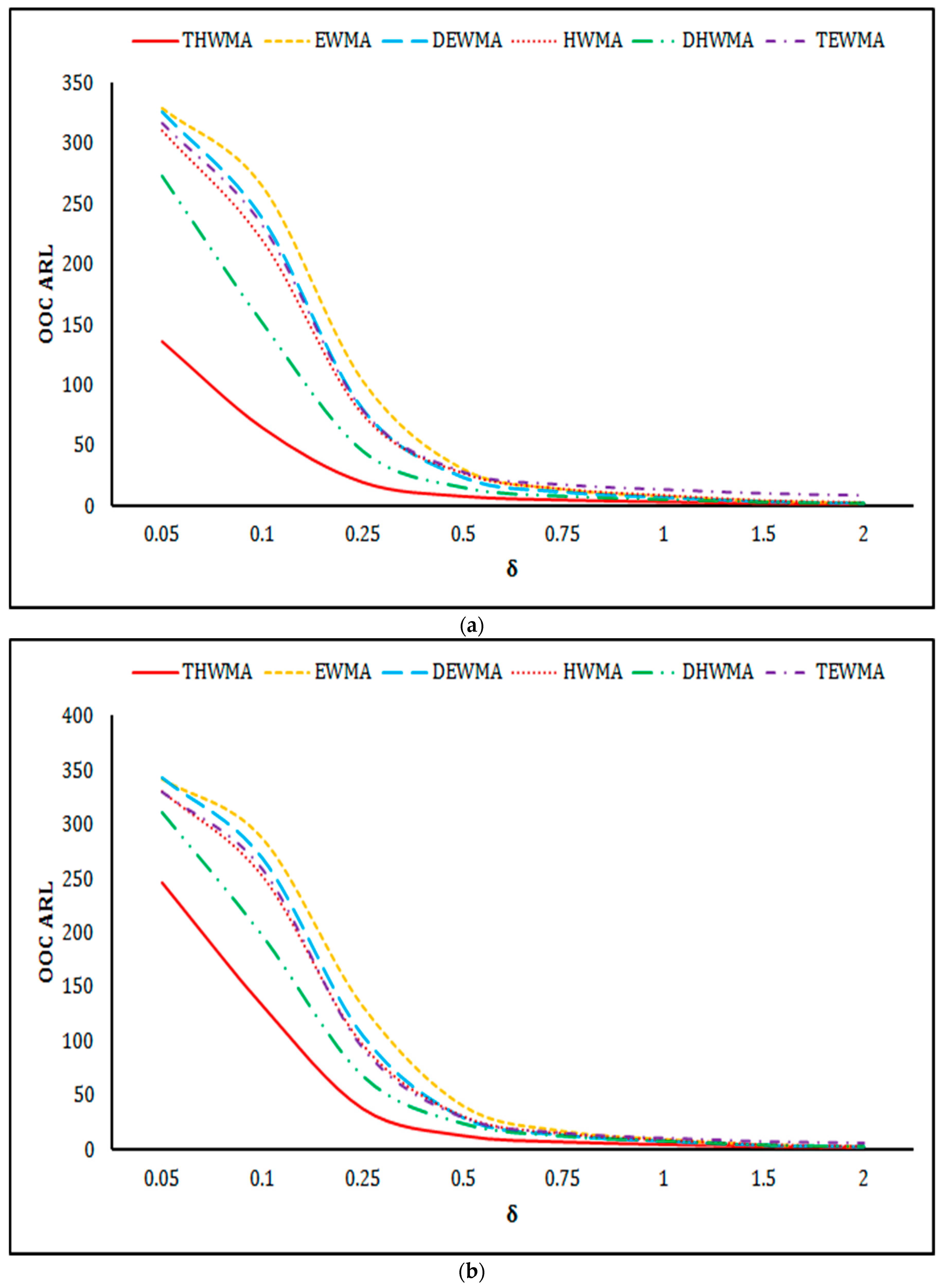
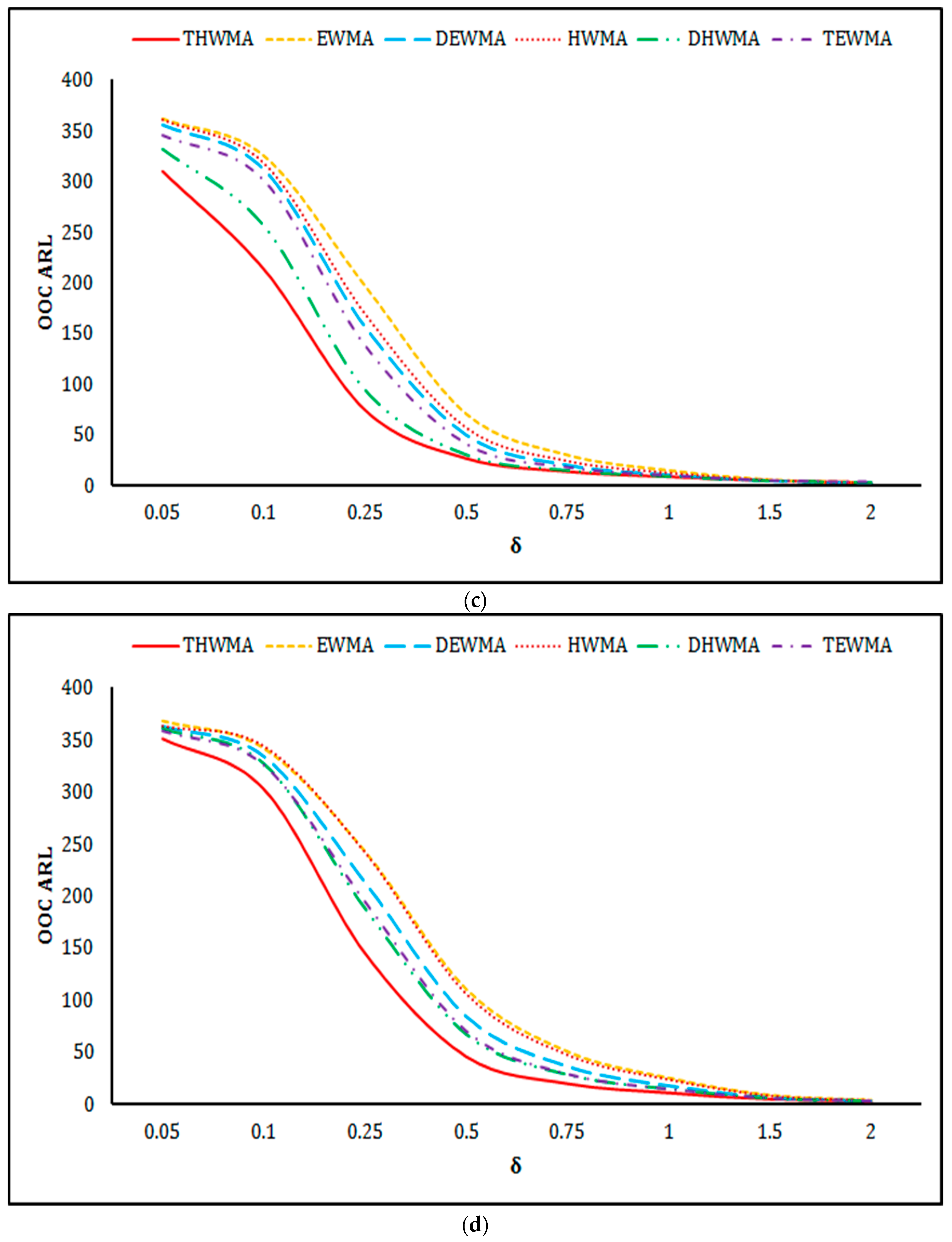
For assessment of the OOC performance between the proposed THWMA and existing charts, line graphs are provided at various combinations of design parameters between shifts and corresponding OOC ARL. A chart is considered superior if its OOC curve is on the lower side, corresponding to certain shifts as compared to competitors. All the curves of proposed and existing competitors are presented in Figure 2. From Figure 2, the performance of the proposed THWMA scheme can be found far better than all the competitors at small and median shifts in the process, particularly at small choices of design parameters. In small values of design parameters, the DHWMA chart is second in its performance and HWMA seems to be third, but as the smoothing parameter increases, TEWMA becomes the third efficient chart among all the competitors.

4. Application of the Proposed THWMA and Existing Charts

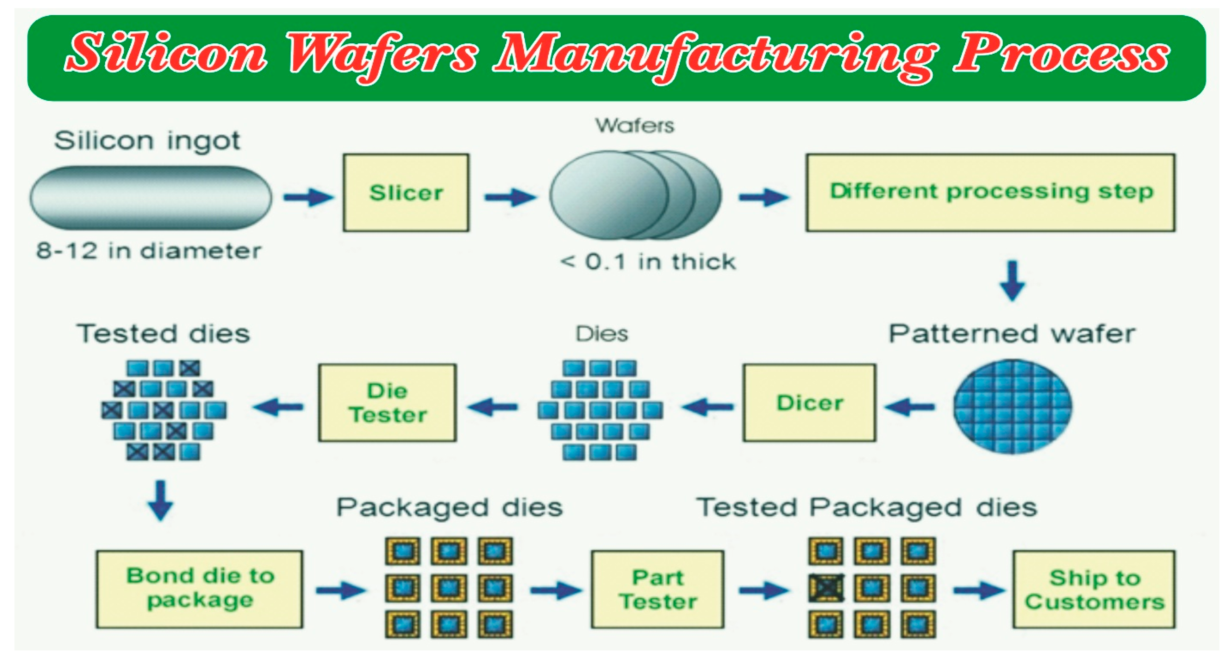
To apply the proposed THWMA scheme to a real dataset application, this section presents an illustration of the proposal with existing HWMA and DHWMA charts. The real dataset related to the industrial manufacturing process is adopted from Montgomery [3]. Silicon wafers are well-known as silicon chips or silicon slices. These are very thin slices of purest monocrystalline that are usually used in tablets, smartphones, laptops, computers, numerous home appliances, artificial intelligence, robotics, autonomous (self-driving cars), fabricated integrated circuits, transistors, solar cells, semiconductors, etc. The dataset related to the manufacturing of semiconductors is taken into account in this study from Montgomery [3] from which flow width of the resistance (FWR) is taken as a key quality characteristic. The manufacturing process is presented in Figure 3.

The FWR has been measured using a subgroup size of 5 after every hour. The dataset consists of 45 sample numbers from which the first 25 samples are considered from the IC process, and the next 20 contain an upward shift. The estimated mean and standard deviation from the first 25 samples are 1.50562 and 0.139425, respectively. Based on these estimated parameters, control limits are set for monitoring the next 20sample observations.

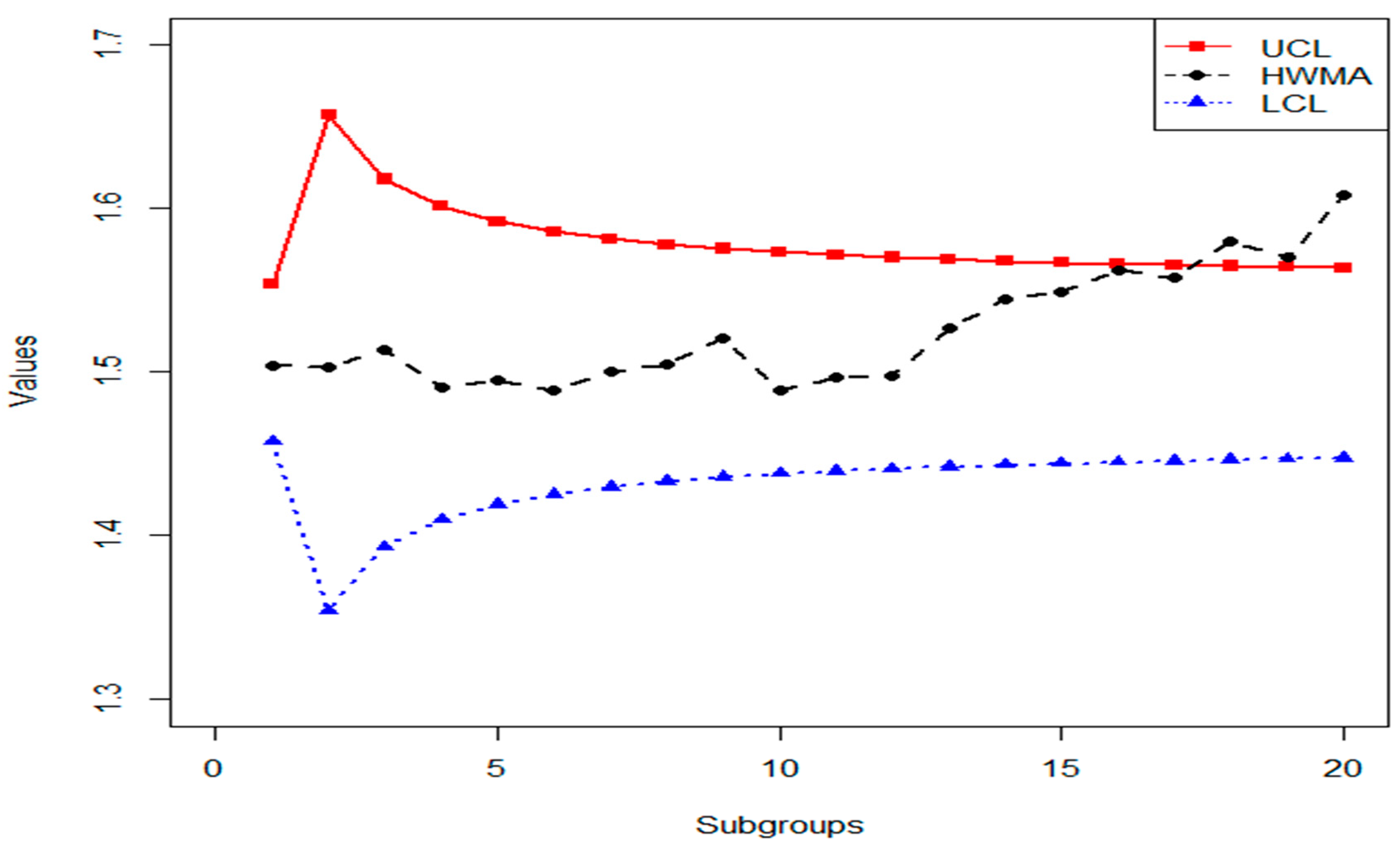
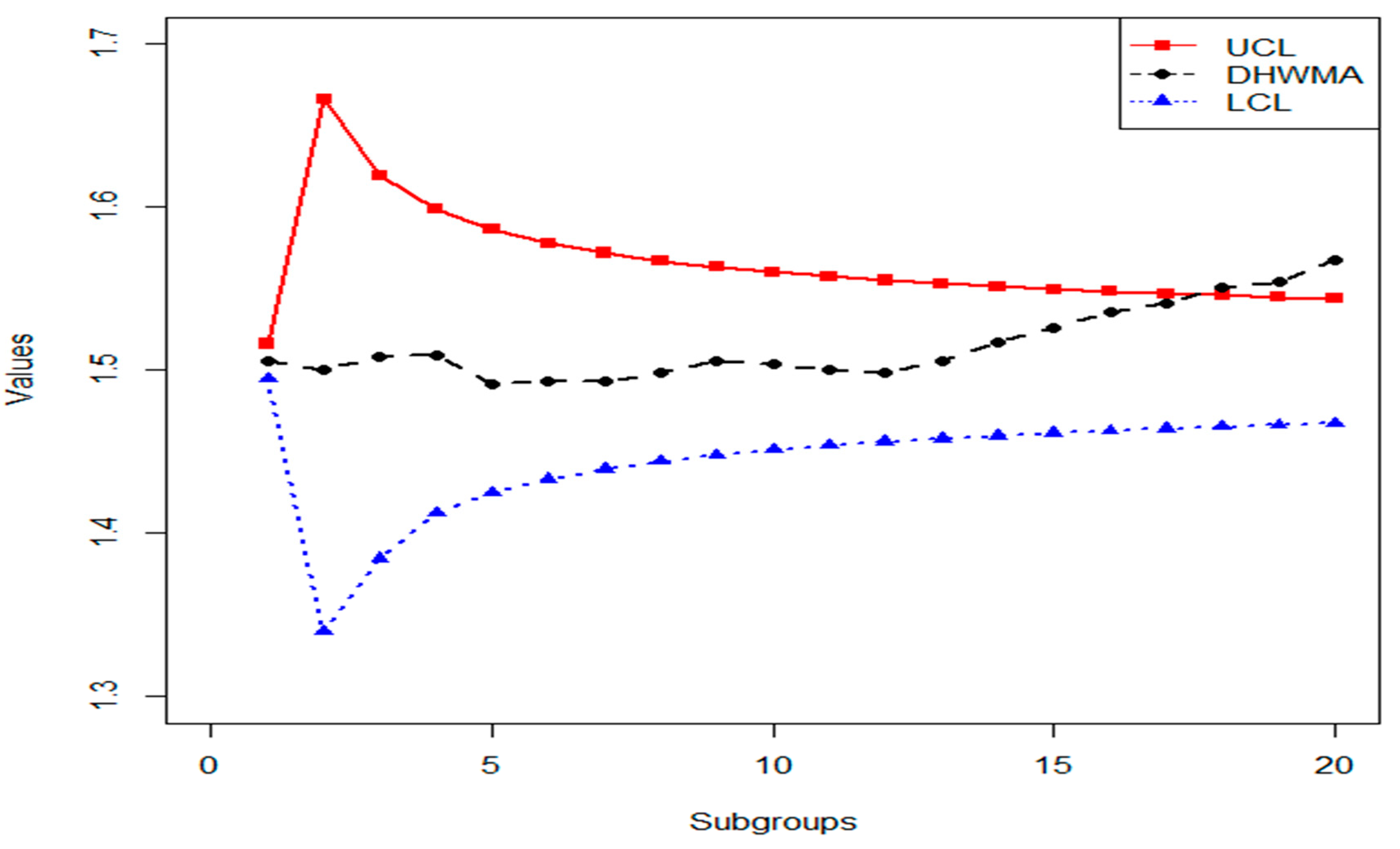
For implementation purposes in this section, the proposed THWMA chart along with HWMA and DHWMA charts are considered. For HWMA scheme design parameters $\lambda =0.25$ and $K=3.075$, for DHWMA chart design parameters $\lambda =0.25$ and $K=3.7424$, and for the proposed THWMA model design parameters $\lambda =0.25$ and $K=2.994$ are taken into account at the desired IC $AR{L}_0\approx 370$ for all the charts. The graphical presentations of the proposed and existing counterparts are presented in Figure 4, Figure 5 and Figure 6. The HWMA and DHWMA charts trace an upward trend at sample number 18 (cf. Figure 4 and Figure 5) and the proposed THWMA scheme triggers the shift at the 17th sample point (cf. Figure 6). This illustrative section narrates that the proposed THWMA chart has a higher detection ability than its competitors in identifying shifts.

5. Concluding Remarks

To produce products at a large scale with high quality, the manufacturing industries are relying on heavy machinery. Variations exist in ongoing production and manufacturing processes. The variations that are an inherent part of every process are natural causes of variations, and the variations that deprive the process of the required quality of output are assumed as special causes of variations. SPM provides a toolkit for improving the processes by identifying special causes of variation from the ongoing process. The control charting schemes are the most famous and widely used SPM tool monitoring and improving the running processes. In this study, an advanced charting scheme, namely, the THWMA chart, has been proposed under zero and steady-state modes. The RL profiles of the proposed THWMA chart at various combinations of design parameters under both states are evaluated. The steady-state case was found superior as compared to zero-state, particularly at small choices of the smoothing parameter. The robustness against non-normal process distributions is also incorporated in this study for the proposed design for the heavy-tailed, symmetric, highly skewed, and contaminated normal distributions. It is found that at large choices of smoothing constant, non-normality assumption affects the IC performance of the proposed THWMA chart. The OOC performance of the proposed scheme is compared with many existing structures in literature and found to be superior for tracing small to medium shifts. An illustrative example related to the manufacturing process of silicon wafers is also provided to highlight the importance of the proposal.

The proposal can be extended for monitoring variability, joint monitoring, and profile monitoring under univariate and multivariate structures using various sampling techniques.

References

- Page, E.S. Continuous inspection schemes. Biometrika 1954, 41, 100–115. [Google Scholar] [CrossRef]
- Roberts, S. Control chart tests based on geometric moving averages. Technometrics 1959, 42, 239–250. [Google Scholar] [CrossRef]
- Montgomery, D.C. Introduction to Statistical Quality Control, 7th ed.; John Wiley & Sons: New York, NY, USA, 2012. [Google Scholar]
- Abbas, N. Homogeneously weighted moving average control chart with an application in substrate manufacturing process. Comput. Ind. Eng. 2018, 120, 460–470. [Google Scholar] [CrossRef]
- Lucas, J.M. Combined Shewhart-CUSUM quality control schemes. J. Qual. Technol. 1982, 14, 51–59. [Google Scholar] [CrossRef]
- Lucas, J.M.; Saccucci, M.S. Exponentially weighted moving average control schemes: Properties and enhancements. Technometrics 1990, 32, 1–12. [Google Scholar] [CrossRef]
- Runger, G.C.; Montgomery, D.C. Adaptive sampling enhancements for Shewhart control charts. IIE Trans. 1993, 25, 41–51. [Google Scholar] [CrossRef]
- Shamma, S.E.; Shamma, A.K. Development and evaluation of control charts using double exponentially weighted moving averages. Int. J. Qual. Reliab. Manag. 1992, 9, 18–25. [Google Scholar] [CrossRef]
- Abbas, N.; Riaz, M.; Does, R.J. Mixed exponentially weighted moving average–cumulative sum charts for process monitoring. Qual. Reliab. Eng. Int. 2013, 29, 345–356. [Google Scholar] [CrossRef]
- Zaman, B.; Riaz, M.; Abbas, N.; Does, R.J. Mixed cumulative sum–exponentially weighted moving average control charts: An efficient way of monitoring process location. Qual. Reliab. Eng. Int. 2015, 31, 1407–1421. [Google Scholar] [CrossRef]
- Abbas, Z.; Nazir, H.Z.; Akhtar, N.; Riaz, M.; Abid, M. An enhanced approach for the progressive mean control charts. Qual. Reliab. Eng. Int. 2019, 35, 1046–1060. [Google Scholar] [CrossRef]
- Abbas, Z.; Nazir, H.Z.; Akhtar, N.; Riaz, M.; Abid, M. On developing an exponentially weighted moving average chart under progressive setup: An efficient approach to manufacturing processes. Qual. Reliab. Eng. Int. 2020, 36, 2569–2591. [Google Scholar] [CrossRef]
- Riaz, M.; Abbas, Z.; Nazir, H.Z.; Akhtar, N.; Abid, M. On Designing a Progressive EWMA Structure for an Efficient Monitoring of Silicate Enactment in Hard Bake Processes. Arab. J. Sci. Eng. 2020. [Google Scholar] [CrossRef]
- Abid, M.; Shabbir, A.; Nazir, H.Z.; Sherwani, R.A.K.; Riaz, M. A double homogeneously weighted moving average control chart for monitoring of the process mean. Qual. Reliab. Eng. Int. 2020, 36, 1513–1527. [Google Scholar] [CrossRef]
- Raza, M.A.; Nawaz, T.; Han, D. On Designing Distribution-Free Homogeneously Weighted Moving Average Control Charts. J. Test. Eval. 2020, 48, 3154–3171. [Google Scholar] [CrossRef]
- Aslam, M.; Rao, G.S.; Al-Marshadi, A.H.; Jun, C.-H. A Nonparametric HEWMA-p Control chart for variance in monitoring processes. Symmetry 2019, 11, 356. [Google Scholar] [CrossRef] [Green Version]
- Chen, J.-H.; Lu, S.-L. A New Sum of Squares Exponentially Weighted Moving Average Control Chart Using Auxiliary Information. Symmetry 2020, 12, 1888. [Google Scholar] [CrossRef]
- Alevizakos, V.; Chatterjee, K.; Koukouvinos, C. The triple exponentially weighted moving average control chart. Qual. Technol. Quant. Manag. 2020. [Google Scholar] [CrossRef]
- Shewhart, W.A. Quality control charts. Bell Syst. Tech. J. 1926, 5, 593–603. [Google Scholar] [CrossRef]
- Abbasi, S.A. On the performance of EWMA chart in the presence of two-component measurement error. Qual. Eng. 2010, 22, 199–213. [Google Scholar] [CrossRef]
- Hussain, S.; Mei, S.; Riaz, M.; Abbasi, S.A. On Phase-I Monitoring of Process Location Parameter with Auxiliary Information-Based Median Control Charts. Mathematics 2020, 8, 706. [Google Scholar] [CrossRef]
- Graham, M.A.; Chakraborti, S.; Human, S.W. A nonparametric EWMA sign chart for location based on individual measurements. Qual. Eng. 2011, 23, 227–241. [Google Scholar] [CrossRef]
- Abbas, Z.; Nazir, H.Z.; Akhtar, N.; Abid, M.; Riaz, M. On designing an efficient control chart to monitor fraction nonconforming. Qual. Reliab. Eng. Int. 2020, 36, 547–564. [Google Scholar] [CrossRef]
- Radson, D.; Boyd, A.H. Graphical representation of run length distributions. Qual. Eng. 2005, 17, 301–308. [Google Scholar] [CrossRef]
- Rocke, D.M. Robust control charts. Technometrics 1989, 31, 173–184. [Google Scholar] [CrossRef]
- Human, S.W.; Kritzinger, P.; Chakraborti, S. Robustness of the EWMA control chart for individual observations. J. Appl. Stat. 2011, 38, 2071–2087. [Google Scholar] [CrossRef] [Green Version]
- Steiner, S.H. EWMA control charts with time-varying control limits and fast initial response. J. Qual. Technol. 1999, 31, 75–86. [Google Scholar] [CrossRef]
- Zhang, L.; Chen, G. An extended EWMA mean chart. Qual. Technol. Quant. Manag. 2005, 2, 39–52. [Google Scholar] [CrossRef]
Figure 1.
The out-of-control (OOC) ARL performance of the proposed for a different choice of under (a) zero-state (b) steady-state.
Figure 2.
The OOC ARL performance of the proposed and existing chart for (a) (b) (c) and (d) .
Figure 3.
A pictorial display of Silicon Wafer Manufacturing procedure.
Figure 4.
Real-life application of the HWMA chart for and .
Figure 5.
Real-life application of the DHWMA chart for and .
Figure 6.
Real-life application of the THWMA chart for and .