On Present Value Evaluation under the Impact of Behavioural Factors Using Oriented Fuzzy Numbers

Abstract

In general, the present value (PV) concept is ambiguous. Therefore, behavioural factors may influence on the PV evaluation. The main aim of our paper is to propose some method of soft computing PV evaluated under the impact of behavioural factors. The starting point for our discussion is the notion of the Behavioural PV (BPV) defined as an imprecisely real-valued function of distinguished variables which can be evaluated using objective financial knowledge or subjective behavioural premises. In our paper, a BPV is supplemented with a forecast of the asset price closest to changes. Such BPV is called the oriented BPV (O-BPV). We propose to evaluate an O-BPV by oriented fuzzy numbers which are more useful for portfolio analysis than fuzzy numbers. This fact determines the significance of the research described in this article. O-BPV may be applied as input signal for systems supporting invest-making. We consider here six cases of O-BPV: overvalued asset with the prediction of a rise in its price, overvalued asset with the prediction of a fall in its price, undervalued asset with the prediction of a rise in its price, undervalued asset with the prediction of a fall in its price, fully valued asset with the prediction of a rise in its rice and fully valued asset with the prediction of a fall in its rice. All our considerations are illustrated by numerical examples. Presented examples show the way in which we transform superposition of objective market knowledge and subjective investment opinion into simple return rate.

1. Introduction

The starting point for evaluating any financial asset is its present value (PV), defined as a current equivalent of a cash payable in a fixed moment of the future [1]. It results in the fact that the PV of a future cash flows may be an imprecise value. For this reason, the reliable PV evaluation requires the use of soft computing a commonly accepted model of an imprecise value is a fuzzy number (FN) [2]. The natural consequence of this approach is estimating PV with FNs. Therefore, fuzzy PV may be defined as a discounted fuzzy prediction of a future cash flow value [3].

The concept of using FNs in financial arithmetic comes from Buckley [4]. The Ward’s definition [3] was generalized in [5] to the case of imprecisely assessed postponement. Sheen [6] expanded the Ward’s definition to the case of fuzzy interest rate. The problems connected to calculating fuzzy PV were considered in [4,7,8,9]. Huang [10] expanded the Ward’s definition to the case of future cash flow described by a fuzzy variable. A more general definition of fuzzy PV was proposed by Tsao [11], who assumed that future cash flow can be treated as a fuzzy probabilistic set. Calzi [12] has formulated an axiomatic definition of fuzzy PV. All those authors depicted PV as a discount of an imprecisely evaluated future cash flow. A different approach was introduced in [13], where the fuzzy PV is determined as imprecise approximation of the current quoted price of an evaluated asset. Some applications of fuzzy PV were considered in [12,13,14,15,16,17,18]. FNs are also used in quantitative finance for modelling imprecision of financial data. In most of the papers regarding imprecision in finance, it is assumed a priori that the return rate from a security is a FN [19,20,21,22,23,24,25,26,27,28,29]. Yet, this assumption is connected, in most cases, to uncertain or unclear or incomplete information available to the investor. Then, authors apply mostly possibility theory [30,31] and credibility theory [32]. Kahraman et al. [33] introduced a research in which both cash flows and return rates are evaluated by trapezoidal FNs. Limiting them to the case of trapezoidal FNs stems from the fact that arithmetic for trapezoidal FNs is significantly simpler than arithmetic for any FNs. More information on this topic is presented in competent monographies [34,35].

Ordered FNs are defined by Kosiński et al. [36], who in this way introduced a FN additionally equipped with an orientation. For formal reasons [37], the Kosiński’s theory was revised in [38]. If ordered FN is linked to the revised theory, then it is called Oriented FN (OFN) [39,40,41,42]. Ordered FNs are applied in decision-making, economics and finance [42,43,44,45,46,47,48,49,50,51,52,53,54,55,56,57,58,59,60,61,62,63].

In [1,64], the behavioural PV (BPV) was defined as fair price approximation determined under impact of behavioural factors. Then, BPV is imprecisely estimated by FN. In [65], the BPV is supplemented with a qualitative prediction of the price trend. This subjective prediction is implemented in a BPV model as an orientation of FN. The existence of such forecasts is proved by the observed balance between the supply and demand reported by investors in financial markets. In this way, the BPV was replaced by oriented BPV (O-BPV) described by an ordered FN. This approach makes portfolio analysis difficult [57]. These difficulties arise from the fact that the sum of the FNs may, in fact, not be an ordered FN.

For this reason, in this paper we present a revised approach to O-BPV. Our main goal is to describe O-BPV by means of OFNs. In the future, this approach will facilitate portfolio analysis because of OFNs are more useful for portfolio analysis than FNs. Therefore, we intend to apply O-BPV for management of portfolio risk of imprecision determined by some behavioural factors. Such possibilities of future applications determine the significance of the studies described in this work.

In [65], the O-BPV is determined with use ordered FNs. Moreover, its membership function was described by a logically complicated system of identities. This also caused very difficult application of the proposed O-BPV model. Therefore, we will try to simplify the identities describing the O-BPV membership function.

This paper is organised as follows. Behavioural aspects of PV definition are presented in Section 2. Section 3 contains basic information of OFNs. In Section 4, we explain the notion of oriented fuzzy PV. BPV is generally defined in Section 5. An interval representation of BPV is described in Section 6. Fuzzy representation of BPV is discussed in Section 7. The concept of O-BPV is introduced in Section 8. Some examples of O-BPV applications are presented in Section 9. There, O-BPV is used for determining return rate. Section 10 contains final conclusions.

2. Behavioural Essence of Present Value

Any PV is used for discounting the money value. This is the basic tool of financial arithmetic. The starting point for the financial arithmetic development was the interest theory. Development of the financial arithmetic theory has resulted in axioms formulated by Peccati, who has defined PV as an additive function of the payment value [66]. This theory is developed in recent years [67].

Among other things, it has been proved that any PV fulfils the conditions of Peccati’s definition if and only if it is a linear discount [66], meaning that this PV can be represented by the product of the payment value and the discounting factor defined as a nonincreasing function of the payment time. On the basis of the interest theory, assuming constant interest rate, we meet only with exponential discount factors. It has been shown that any compound discount is represented by an exponential discounting factor.

On the other hand, many different kinds of discounting factors were described during the study on a behavioural aspects of dynamic money evaluation. The first mathematical model of behavioural finance was introduced by Ramsey [68], who explained the relationship between the marginal product of capital value, the subjective discount rate and the real interest rate. Samuelson [69] introduced an exponential model of the subjective discount factor. This model was adjusted in [70].

The Samuelson’s model [69] assumes that the subjective discount rate is constant over time. This assumption is one of the many criticised problems of the exponential model. The exponential discount model has “anomalies” related to the behavioural effect that subjective discount rate varies in time [71,72,73,74]. Dynamically inconsistent time preferences with this effect are described in [75,76].

Imperfections of the exponential discounting were found, causing the creation of new discounting models and approaches. The hyperbolic discounting was introduced by Mazur [77] who generalised some particular function applied in [78,79]. Some kinds of discount hyperbolic models are discussed in [73,80]. In [81], we can find arithmetic discounting. This discounting describes bill discounting method specified by financial law. The hyperbolic discounting was generalised to hyperboloid one in [72]. Quasi-hyperbolic discounting [82] is used by economists hoping to preserve as much of the exponential model as possible. In the discrete time version this discounting method was introduced in [83]. The quasi-hyperbolic discounting can also be used for the case of continuous time [84]. Moreover, as an alternative to the percentage decrement for delayed payments may be used a fixed cost model to exponential discounting [84]. Some authors [82,85,86,87,88,89,90,91,92] consider it to be important to extend the hyperbolic function by the behavioural exponents. Very frequently, those models are only some modifications of hyperbolic or exponential discounting.

Hyperbolic models are also criticised (see, for example, in [75,76,92]). Read [92] proposed his model as such exponential discounting that the discount factor occurs within the given time window. Arguing with Weber–Fechner Law [93], Roelofsma [89] proposed his model as an exponential discounting where the exponent is directly proportional to logarithm of time. Ebert and Prelec [90] defined their Constant Sensitivity discounting factor as the Cobb–Douglas function. The Constant Relative Decreasing Impatience discount factor is defined as the constant relative risk aversion function [94]. In an analogous way, Constant Absolute Decreasing Impatience discount factor is defined as a constant absolute risk aversion function [94]. In [81], a discount factor is defined by means of the assumption that its marginal change follows the Stevens’ power law [95,96] which says that “a psychologically effective variable is a power function of its physical cause”. Multi-threaded results of studies on the discounting factors were competently discussed in [80]. Moreover, in [97,98,99] the discount factor is defined for such discounting under continuous capitalisation which is determined by a constant Arrow-Pratt’s measure of absolute risk-aversion. The axiomatic theory of discount factors was introduced in [100] and developed in [101]. Rotschedla et al. [102] present such a discounting model that the discounted value is given as a hedonic price dependent on fundamentals. Let us note that PV defined in this way does not meet the axiomatic conditions determined by Peccati for PV.

The variety of discount approaches described above justifies our approach to PV as an ambiguous value.

Let us summarise the PV studies described above. We see that the impact of behavioural premises differentiates the discounting factors used to determine PV. Moreover, Peccati [66] has shown that any PV may be defined by a discounting factor. It means that Peccati’s definition of PV depends on behavioural premises which are always subjective. On the other side, financial arithmetic requires an objective PV definition. Therefore, any PV is defined as a current equivalent of a cash flow [1]. There financial flow utility is set by the multicriteria comparison consisting of temporal preference [103] and wealth preferences. This definition of PV is more general than the Peccati’s definition. The PV determined by Rotschedla et al. [102] fulfil the conditions of a generalised PV. Generalised PV is defined without a discounting factor. Therefore, a generalised PV definition is independent of a priori given behavioural phenomena. For this reason, the notion of generalised PV is a valid tool to study the behavioural impact on a discount.

The research domain of behavioural finance is the paradoxes and anomalies in financial markets, which are difficult to explain based on neoclassical economic theory. Behavioural analysis of financial markets points to the psychological aspect of an investment as the reason for this state of affairs. At present, an extensive bibliography is already devoted to the results of those studies. The consequence of this intensive research is aiming to obtain such formal models which explain behavioural mechanisms of the financial market. Here, we can distinguish a few approaches to this topic.

The most typical behavioural finance model is a formal prospect theory [104,105]. In this theory, a subjective transformation of the objective probability is distinguished as a behavioural basis for investment decisions.

Barberis et al. [106] develop the prospect theory. They additionally point out imprecise estimation of PV, as a result of the subjective approach to security valuation.

Daniel et al. [107] show the diversified responses of individual investors to received information as the reason for the disclosure of the market paradoxes. Assumed lack of the strong effectiveness of the financial market is one of characteristics of this theory.

Hong and Stein [108] describe the investment activity, as the game amongst investors applying fundamental analysis and investors applying technical analysis. This interaction of two rational theories produces such market phenomena, which are paradoxes from a point of view of the economic theory. PV behavioural aspects are enclosed here in the choice of a cognitive strategy.

Behavioural experiments [75,109,110,111] present the regularities of subjective discounting. There it is show that

• the receivables are discounted by a higher discount rate than liabilities and
• smaller amounts are discounted by a lower discount rate than large amounts.

The above behavioural paradoxes may be explained by means of the prospect theory in its final version. Kahneman and Tversky [112] say that any evaluation depends on risk aversion and on loss aversion. The loos aversion implies that the accelerated consumption is less desirable than the delayed one [73,113]. From economical point of view, any receivable may be considered as delated consumption. In analogous way, any liability can be interpreted as accelerated consumption. It explains why we discount liabilities less than receivable. Unfortunately, this explanation is not sufficient for determining such discounting functions which differentiate the receivable discount and liability discount. Behavioural analysis of financial markets points to the psychological aspect of investors’ activities as the reason for this state of affairs. The behavioural impact on PV has been confirmed by experiments [81,88,113,114,115].

In the general case, each of Peccati’s models of PV [66] is inconsistent with the results of behavioural experiments which explain the financial practice. The subject of behavioural finance research is the phenomena which are paradoxes, inter alia, from the viewpoint of the interest theory. This intensive research consequence is prospecting for such formal models which explain the observed paradoxes.

In recent years, the concept of financial flow utility has played an important role in the behavioural finance research. This problem is discussed, for example, in [73,80,81,116,117,118,119,120,121]. PV is defined there as the financial flow utility. As we see, the behavioural approach to PV is similar to the neoclassical one. All PV models mentioned in this paragraph meet the conditions of a generalised PV definition [1]. In this definition, the financial flow utility is defined in a such way that the receivable utility is positive and the liabilities utility is negative. Therefore, generalised PV may be applied for evaluation of behavioural asymmetry between receivable discount and liability discount described in [73,75,109,110,111,113]. Note that the notion of the negative utility was introduced only by Rabin [122]. All above references prove that many researchers accept the view that the behavioural factors have an impact on evaluating PV.

In [13,64], the BPV was defined as fair price approximation determined under impact of behavioural factors. Such an approach is in line with the approach proposed later by Rotschedla et al. [102]. It causes that any PV estimation is in fact an imprecise number. Because FN is a commonly accepted model of an imprecise number, BPV should be described by an FN.

3. Oriented Fuzzy Numbers—Basic Facts

The symbol $ℱ(ℝ)$ denotes the family of all fuzzy subsets in the real line $ℝ$. Any fuzzy subset $\mathcal{A}\in ℱ(ℝ)$ is described by its membership function ${\mu }_A\in {\left[0,1\right]}^{ℝ}$, as the set of ordered pairs

$$\mathcal{A}=\left\{\left(x,{\mu }_A\left(x\right)\right);x\in ℝ\right\}.$$

(1)

Among other things, this fuzzy subset $\mathcal{A}$ may be characterised by its support closure ${\left[\mathcal{A}\right]}_{0^{+}}$ given in a following way:

$${\left[\mathcal{A}\right]}_{0^{+}}=\underset{\alpha \to 0^{+}}{\lim }\left\{x\in ℝ: {\mu }_A\left(x\right)\ge \alpha \right\}.$$

(2)

FN is usually defined as a fuzzy subset of the real line $ℝ$. The most general definition of FN is given as follows.

Definition 1.

[2] The fuzzy number (FN) is such a fuzzy subset$ℒ\in ℱ(ℝ)$with bounded support closure${[ℒ]}_{0^{+}}$that it is represented by its upper semi-continuous membership function${\mu }_L\in {\left[0;1\right]}^{ℝ}$satisfying the conditions

$${\exists }_{x\in ℝ} {\mu }_L\left(x\right)=1,$$

(3)

$${\forall }_{\left(x,y,z\right)\in {ℝ}^3} x\le y\le z\Rightarrow {\mu }_L\left(y\right)\ge \min \left\{{\mu }_L\left(x\right);{\mu }_L\left(z\right)\right\}.$$

(4)

The set of all FN we denote by the symbol$\mathbb{F}$.

Theorem 1.

[123,124] For any FN$ℒ$there exists such a non-decreasing sequence$\left(a,b,c,d\right) \subset ℝ$that$ℒ\left(a,b,c,d,L_L,R_L\right)=ℒ\in ℱ(ℝ)$is determined by its membership function${\mu }_L\left(x|a,b,c,d,L_L,R_L\right)\in {\left[0,1\right]}^{ℝ}$described by the identity

$${\mu }_L\left(x|a,b,c,d,L_L,R_L\right)=\{\begin{array}{c} 0, x\notin \left[a,d\right],\\ L_L\left(x\right), x\in \left[a,b\right[,\\ 1, x\in \left[b,c\right],\\ R_L\left(x\right), x\in \left]c,d\right], \end{array}$$

(5)

where the left reference function$L_L\in {\left[0,1\right[}^{\left[a,b\right[}$and the right reference function$R_L\in {\left[0,1\right[}^{\left]c,d\right]}$are upper semi-continuous monotonic ones meeting the condition

$${[ℒ]}_{0^{+}}=\left[a,d\right].$$

(6)

The FN $ℒ\left(a,a,a,a,L_L,R_L\right)=〚a〛$ represents the real number $a\in ℝ$. Therefore, we can say $ℝ\subset \mathbb{F}$.

Any function $G:ℝ\supset \mathbb{A}\to ℝ$ may be considered as an unary operator on real numbers. Using the Zadeh’s extension principle, we can extend this operator to the fuzzy case. Let us write this extended operator as the function $\tilde{G}:\mathbb{F}\supset \mathbb{D}\to \mathbb{F}$ described by the equation

$$\mathcal{K}\left(e,f,g,h,L_K,R_K\right)=\tilde{G}\left(ℒ\left(a,b,c,d,L_L,R_L\right)\right),$$

(7)

where

• FN $ℒ\left(a,b,c,d,L_L,R_L\right)$ is represented by its membership function

  $${\mu }_L\left(x\right)={\mu }_L\left(x|a,b,c,d,L_L,R_L\right),$$

  (8)
• FN $\mathcal{K}\left(e,f,g,h,L_K,R_K\right)$ is represented by its membership function

  $${\mu }_K\left(x\right)={\mu }_K\left(x|e,f,g,h,L_K,R_K\right).$$

  (9)

In line with the Zadeh extension principle, the unary operator (7) is uniquely defined by its membership function ${\mu }_K\in {\left[0,1\right]}^{ℝ}$ given by the identity

$${\mu }_K\left(x\right)=\min \left\{\max \left\{{\mu }_L\left(y\right)\right\} : y=G\left(x\right)\right\}.$$

(10)

Moreover, the following concepts may be applied for description of the unary operator (7) in detail.

Definition 2.

[124] For any upper semi-continuous non-decreasing function$L\in {\left[0, 1\right]}^{\left[u, v\right]}$, its cut-function$L^{\star }\in {\left[u,v\right]}^{\left[0;1\right]}$is determined by the identity

$$L^{\star }\left(\alpha \right)=\min \left\{x\in \left[u,v\right]: L\left(x\right)\ge \alpha \right\}.$$

(11)

Definition 3.

[124] For any upper semi-continuous non-increasing function$R\in {\left[0, 1\right]}^{\left[u, v\right]}$, its cut-function$R^{\star }\in {\left[0, 1\right]}^{\left[u, v\right]}$is determined by the identity

$$R^{\star }\left(\alpha \right)=\max \left\{x\in \left[u,v\right]: R\left(x\right)\ge \alpha \right\}.$$

(12)

Definition 4.

[124] For any bounded continuous and non-decreasing function$l\in {\left[l\left(0\right), l\left(1\right)\right]}^{\left[0,1\right]}$, its pseudo-inverse$l^{⊲}\in {\left[0,1\right]}^{\left[l\left(0\right), l\left(1\right)\right]}$is determined by the identity

$$l^{⊲}\left(x\right)=\max \left\{\alpha \in \left[0,1\right]:l\left(\alpha \right)=x\right\}.$$

(13)

Definition 5.

[124] For any bounded continuous and non-increasing function$r\in {\left[r\left(0\right), r\left(1\right)\right]}^{\left[0,1\right]}$, its pseudo-inverse$r^{⊲}\in {\left[0;1\right]}^{\left[r\left(1\right), r\left(0\right)\right]}$is determined by the identity

$$r^{⊲}\left(x\right)=\min \left\{\alpha \in \left[0,1\right]:r\left(\alpha \right)=x\right\}.$$

(14)

Using the theorems proved by Goetschel and Voxman [124], we can show that if the unary operator $G:ℝ\supset \mathbb{A}\to ℝ$ is decreasing, then the unary operator (7) is given by the identity

$$ℒ\left(G\left(d\right),G\left(c\right),G\left(b\right),G\left(a\right),L_K,R_K\right)=\tilde{G}\left(ℒ\left(a,b,c,d,L_L,R_L\right)\right),$$

(15)

where

$${\forall }_{\alpha \in \left[0,1\right]} l_K\left(\alpha \right)=G\left(L_L^{\star }\left(\alpha \right)\right),$$

(16)

$${\forall }_{\alpha \in \left[0,1\right]} r_K\left(\alpha \right)=G\left(R_L^{\star }\left(\alpha \right)\right),$$

(17)

$${\forall }_{y\in \left[G\left(d\right),G\left(c\right)\right[} L_K\left(y\right)=r_K^{⊲}\left(y\right),$$

(18)

$${\forall }_{y\in \left]G\left(b\right),G\left(a\right)\right]} R_K\left(y\right)=l_K^{⊲}\left(y\right).$$

(19)

The notion of ordered FN is introduced by Kosiński et al. [36]. An important disadvantage of Kosiński’s theory is that there exist such ordered FNs which are not linked to any membership function [37]. For formal reasons, the Kosiński’s theory is revised in [38]. In revised theory, ordered FN is replaced by oriented FN (OFN) defined as follows.

Definition 6.

[38] For any monotonic sequence$\left(a,b,c,d\right)\subset ℝ$, OFN$\overleftrightarrow{ℒ}\left(a,b,c,d,S_L,E_L\right)=\overleftrightarrow{ℒ}$is the pair of orientation$\overrightarrow{a,d}=\left(a,d\right)$and FN described by membership function${\mu }_L\left(\cdot |a,b,c,d,S_L,E_L\right)\in {\left[0,1\right]}^{ℝ}$given by the identity

$${\mu }_L\left(x|a,b,c,d,S_L,E_L\right)=\{\begin{array}{c} 0, x\notin \left[a,d\right]\equiv \left[d,a\right],\\ S_L\left(x\right), x\in \left[a,b\right[\equiv \left]b,a\right],\\ 1, x\in \left[b,c\right]\equiv \left[c,b\right] ,\\ E_L\left(x\right), x\in \left]c,d\right]\equiv \left[d,c\right[,\end{array}$$

(20)

where the starting function$S_L\in {\left[0,1\right[}^{\left[a,b\right[}$and the ending function$E_L\in {\left[0,1\right[}^{\left]c,d\right]}$are upper semi-continuous monotonic ones meeting the condition (6).

The identity (20) additionally describes such modified notation of intervals which is used in the OFN theory. The notation $ℐ\equiv \mathcal{K}$ means that “the interval $ℐ$ may be equivalently replaced by the interval $\mathcal{K}$”.

The symbol $\mathbb{K}$ denotes the space of all OFNs. Any OFN describes an imprecise number with additional information about the location of the approximated number. This information is given as an orientation of OFN. If $a<d$, then OFN $\overleftrightarrow{ℒ}\left(a,b,c,d,S_L,E_L\right)$ has the positive orientation $\overrightarrow{a,d}$. If $a>d$, then OFN $\overleftrightarrow{ℒ}\left(a,b,c,d,S_L,E_L\right)$ has the negative orientation $\overrightarrow{a,d}$. If $a=d$, OFN $\overleftrightarrow{ℒ}\left(a,a,a,a,S_L,E_L\right)=〚a〛$ describes an unoriented number $a\in ℝ$.

Kosiński has defined arithmetic operators on ordered FNs in an intuitive way consistent with the results obtained by Goetschel and Voxman [124]. For OFNs, any arithmetic operator is defined alike. In this way, any unary operator $G:ℝ\supset \mathbb{A}\to ℝ$ may be extended to OFN case. Using the Kosiński’s approach, we define an extended unary operator $\overleftrightarrow{G}:\mathbb{K}\supset ℍ\to \mathbb{K}$ as follows:

$$\overleftrightarrow{\mathcal{K}}\left(G\left(a\right),G\left(b\right),G\left(c\right),G\left(d\right),S_K,E_K\right)=\overleftrightarrow{G}\left(ℒ\left(a,b,c,d,S_L,E_L\right)\right),$$

(21)

where

$$\forall \alpha \in \left[0,1\right] s_K\left(\alpha \right)=G\left(S_L^{\star }\left(\alpha \right)\right),$$

(22)

$$\forall \alpha \in \left[0,1\right] e_K\left(\alpha \right)=G\left(E_L^{\star }\left(\alpha \right)\right),$$

(23)

$$\forall y\in \left[G\left(a\right),G\left(b\right)\right[ S_K\left(y\right)=s_K^{⊲}\left(y\right),$$

(24)

$$\forall y\in \left]G\left(c\right),G\left(d\right)\right] E_K\left(y\right)=e_K^{⊲}\left(y\right).$$

(25)

When we compare the dependencies (15–19) and (21–25), then we notice that for the case of decreasing unary operator $G:ℝ\supset \mathbb{A}\to ℝ$, its extension to OFNs differs from its extension to FNs. This is an important difference between OFNs and FNs.

In Section 8 and Section 9, we restrict our considerations to the case of strictly monotonic starting and ending functions. Then, for any monotonic unary operator $G:ℝ\supset \mathbb{A}\to ℝ$, Equation (21) is simpler because then we have

$$\forall y\in \left[G\left(a\right),G\left(b\right)\right[ S_K\left(y\right)=S_L\left(G^{-1}\left(y\right)\right),$$

(26)

$$\forall y\in \left]G\left(c\right),G\left(d\right)\right] E_K\left(y\right)=E_L\left(G^{-1}\left(y\right)\right).$$

(27)

4. Oriented Fuzzy Present Value

The start point for our considerations is a notion of PV defined as a current equivalent. In Section 2, we have shown that PV may be imprecise. This observation agrees with understanding PV as equivalent of future cash flow. The natural consequence of these conclusions is estimating PV with FNs. Therefore, such PV is called a fuzzy one (F-PV). In Section 1, the evolution of F-PV model is described in detail. In general, fuzzy PV is characterised by a non-decreasing sequence $\left(V_s, V_f, \check{P}, V_l, V_e\right)$, where

• $\check{P}$ is a quoted price,
• $\left[V_s,V_e\right]\subset {ℝ}^{+}$ is an interval of all possible values of PV,
• $\left[V_f,V_l\right]\subset \left[V_s,V_e\right]$ is an interval of all prices which do not noticeably differ from a quoted price $\check{P}$.

Then F-PV is estimated by FN

$$\widetilde{PV}=ℒ\left(V_s, V_f, V_l, V_e ,S_{PV},E_{PV} \right),$$

(28)

where the reference functions $S_{PV}\in {\left[0,1\right[}^{\left[V_s,V_f\right[}$ and $E_{PV}\in {\left[0,1\right[}^{\left]V_l,V_e\right]}$ are the given ones.

Moreover, the F-PV estimation should be supplemented by a forecast of price closest changes. For example, price closes changes may be predicted with the use of prediction table presented in [125]. In [126], it is shown that OFN application for a portfolio analysis is more useful than the analogous application of FN. For these reasons, an imprecise PV may be evaluated by OFN [42,62]. PV determined in this way is called an oriented one (O-PV). Any O-PV is characterised by a monotonic sequence $\left(V_s, V_f, \check{P}, V_l, V_e\right)$ and then it is estimated as follows:

$$\overleftrightarrow{PV}=\overleftrightarrow{ℒ}\left(V_s, V_f, V_l, V_e,L_{PV},R_{PV}\right).$$

(29)

If we predict a increase in price, then O-PV has positive orientation. If we predict a fall in price, then O-PV has a negative orientation.

In this paper, O-PV is used for modelling imprecise assessments of PV. After Klir [127], the imprecision is composed of ambiguity and indistinctness. In the considered case, the ambiguity is understood as a lack of clear indication of a one value out of many. An indistinctness is interpreted as a lack of an explicit distinction between values equal to PV and values different from PV.

5. Behavioural Present Value

Let us consider a fixed asset which is the subject of a trade on a financial market. The quoted price $\check{P}$ of this asset may fluctuate over time. Therefore, we can consider a quotation trend. If the demand for this asset is equal to its supply, then the quoted price $\check{P}$ is equal to balanced price $P_0$. Then, the asset market is balanced, and it meets the market equilibrium condition. In general, the balanced price varies with time. Nevertheless, at any point in time the current value of a balanced price can be determined by the econometric model contained in the Arbitrage Price Theory [128]. In this way, the balanced price $P_0$ may also be substantively justified by fundamental factors. Of course, the balanced price may be computed in a different way. It is important here that the investor accepts the calculated value $P_0$ as the balanced price.

Fama [129] introduces a well-known notion of a market informational efficiency. Then, Fama hypothesises that the highly informationally efficient markets do not exist. In 1980, Grossman and Stiglitz [130] show that information efficiency increases with a decrease in the cost of acquiring and analysing information. Since then, we have been observing the intensive development of computerisation, among others in the economic and financial sphere. This development significantly reduces the cost of processing information. Therefore, today we can assume that the considered asset market is highly informationally efficient. This assumption is consistent with a base of the behavioural finance theory [104,105,112].

Using technical analysis, we assume that the quoted price $\check{P}$ converges to the balanced price P₀. If

$$\check{P}<P_0$$

(30)

then the considered asset is undervalued. For the case

$$\check{P}>P_0$$

(31)

the considered asset is overvalued. We call both of these cases financial disequilibrium states. For the case of financial equilibrium

$$\check{P}=P_0$$

(32)

the considered asset is fully valued.

The accrued market knowledge is the unique basis for determining the value of balanced price $P_0$. This value is a synthetic image of knowledge about the state of financial market. On the highly efficient financial market, each market player determines the same value $P_0$, which is an objective in this situation. At the same time, all investors observe the identical value of quoted price $\check{P}$. Therefore, this value is an objective in its essence. The knowledge of both of these values is sufficient for rational investment-making. In case (30), the rationale suggests buying the considered asset. This transaction is only possible if a sale offer is proposed. The natural question here is, what were the reasons of the investor selling undervalued asset. Similarly, for case (31) the rationale suggests selling the considered financial instrument. This transaction is only possible if a purchase offer is proposed. This raises the question of what were the reasons for the investor buying the valued asset and what premises direct investors buying this security. We discuss above only balancing the demand and supply reported by the investors. Liquidity traders perform their transactions only when this balance vanishes. This phenomenon is widely observed. The answer to the above two questions can be only one. An explanation is only the influence of behavioural factors.

Financial disequilibrium is described by the alternative of inequalities (30) or (31). If a highly efficient financial market is under the financial disequilibrium, then the market equilibrium is maintained due to irrational premises. It causes that every transaction is concluded under the influence of irrational premises. These premises may be behavioural in nature. Therefore, consideration of behavioural factors helps to clarify the paradox of the paradox of maintaining market equilibrium in the conditions of financial disequilibrium in highly efficient market.

The finance theory suggests that PV should be equal to the quoted price $\check{P}$. On the other hand, a balanced price $P_0$ may influence the PV deviation from the observed quoted price. This deviation depends on the investor receptivity to behavioural factors.

Therefore, PV evaluation is determined, inter alia, under the influence of behavioural factors. Each behavioural evaluation is subjective. In Section 2, we have shown that subjective assessment of PV is ambiguous. Each of the valuation alternatives is called a possible PV (PPV). The behavioural PV (BPV) is defined as a convex set of all PPV. According to the classical finance theory, the quoted price $\check{P}$ is also PPV. For this reason, BPV is a strong generalisation of PV model proposed by Rotschedla et al. [102]. The BPV dependence on subjective financial factors means that each investor designates their own version of BPV. Thus, we will conduct all further considerations for the established single investor.

6. Interval Representation of Behavioural Present Value

Any convex crisp subset of real numbers is an interval. For this reason, the subject of our first considerations is BPV represented by an interval.

We begin our considerations on BPV by discussing case (32) of financial equilibrium. This assumption causes that any PPV is approximation of the quoted price $\check{P}$. The considered PPV domain always depends on a specific investor’s susceptibility to the influence of behavioural factors. Therefore, each investor subjectively distinguishes the following values:

• P_min the minimal PPV expected under the financial equilibrium condition (32),
• $P_{max}$ the maximal PPV expected under the financial equilibrium condition (32).

In general, the investor may not be aware of these values. However, when preparing any investment decision support system, we can ask the investor about these values. Therefore, we assume the values $P_{min}$ and $P_{max}$ are known to us.

In the considered case, each investor must take into account the possibility of changes in quotations. Then, the range of PPV variability fulfils the condition

$$0<P_{min}<P_0<P_{max}.$$

(33)

Numerical interval $[P_{min},P_{max}]$ is the BPV image determined for the case of the financial equilibrium.

We lead further considerations on BPV for any quoted price $\check{P}$. Then BPV should be dependent on deviation

$$\Delta P=\check{P}-P_0.$$

(34)

of the quoted price from the balanced price. For each investor, we determine the following values:

• $V_{min}$ the minimal PPV expected for the quoted price $\check{P}$,
• $V_{max}$ the maximal PPV expected for the quoted price $\check{P}$.

In line with Barberis et al. [106], we assume that both values are dependent on the sentiment index $\alpha \in ]0,1]$. We consider sentiment index as an individual investor’s characteristic. The value $\alpha \in ]0,1]$ describes the degree of the influence of cognitive conservatism phenomenon [131]. This phenomenon is a frequent topic of discussion in behavioural finance. The value $1-\alpha \in [0;1[$ informs us about the intensity of the impact of deviation $\Delta P$ on the investor’s beliefs.

The investor determines the minimal PPV $V_{min}$ as the weighted average of the assumed minimal PPV $P_{min}$ and its current correction $P_{min}+\Delta P$. The weight of the minimal PPV $P_{min}$ is equal to the value $\alpha$ of the investor’s sentiment index. In determining the minimal PPV $V_{min}$, the investor must consider that the minimal PPV is not greater than the quoted price $\check{P}$. We get

$$\begin{array}{c}{V}_{min}=\min \left\{\left(1-\alpha \right)·\left(P_{min}+\Delta P \right)+\alpha ·P_{min},\check{P}\right\}=\min \left\{P_{min}+\left(1-\alpha \right)·\Delta P,\check{P}\right\}\\ =\min \left\{P_{min}+\left(1-\alpha \right)·\left(\check{P}-P_0\right),\check{P}\right\}.\end{array}$$

(35)

The investor determines the maximal PPV $V_{max}$, as the weighted average of the assumed maximal PPV $P_{max}$ and its current correction $P_{max}+\Delta P$. The weight of the maximal PPV $P_{max}$ is equal to the value $\alpha$ of the investor’s sentiment index. In determining the maximal PPV $V_{max}$, the investor must consider that the maximal PPV is not less than the quoted price $\check{P}$. We get

$$\begin{array}{c}{V}_{max}=\max \left\{\left(1-\alpha \right)·\left(P_{max}+\Delta P\right)+\alpha ·P_{max},\check{P}\right\}=\max \left\{P_{max}+\left(1-\alpha \right)·\Delta P,\check{P}\right\}\\ =\max \left\{P_{max}+\left(1-\alpha \right)·\left(\check{P}-P_0\right),\check{P}\right\}.\end{array}$$

(36)

We note that in case

$$\check{P}\le \frac{P_{min}-P_0}{\alpha }+P_0$$

(37)

the minimal PPV $V_{min}$ is equal to the quoted price $\check{P}$. Then, the BPV model excludes a possibility of decline in quotation because of the considered asset is uniquely identified as undervalued. Furthermore, when

$$\check{P}\ge \frac{P_{max}-P_0}{\alpha }+P_0$$

(38)

then maximal PPV $V_{max}$ is equal to the quoted price $\check{P}$. Then, the BPV model excludes a possibility of rise in quotation because of the considered asset is uniquely identified as overvalued.

We see that only in the case of large deviations $\Delta P$, rationale is the only reason to invest. Range of behavioural reasons’ impact is described by the inequalities

$$\frac{P_{min}-P_0}{\alpha }+P_0<\check{P}<\frac{P_{max}-P_0}{\alpha }+P_0.$$

(39)

Finally, for each investor we can determine a PPV variability range

$$\overline{BPV}\left(\check{P}\right)=\left[V_{min},V_{max}\right]=\{\begin{array}{l}\left[\check{P}, P_{max}+\left(1-\alpha \right)·\Delta P\right]\hspace{1em}\hspace{1em}\hspace{1em}\hspace{1em}\hspace{1em}\hspace{1em}\hspace{1em}\hspace{1em}for \left(37\right)\\ \left[P_{min}+\left(1-\alpha \right)·\Delta P, P_{max}+\left(1-\alpha \right)·\Delta P\right] \hspace{1em}for \left(39\right)\\ \left[P_{min}+\left(1-\alpha \right)·\Delta P, \check{P}\right] for \left(38\right)\end{array}.$$

(40)

Analogous results were obtained in [63,64,65]. In this way, we have set the image of market information impact on the investor’s beliefs. Determined above range $\left[V_{min},V_{max}\right]$ is an interval representation of BPV (I-BPV) depending on the variables below:

• $\check{P}$ a quoted price,
• $P_0$ a balanced price,
• $P_{min}$ the minimal PPV expected under financial equilibrium condition (32),
• $P_{max}$ the maximal PPV expected under financial equilibrium condition (32),
• $\alpha$ a sentiment index.

The assumed PPV range $\left[P_{min},P_{max}\right]$ and a value of sentiment index $\alpha \in \left]0;1\right]$ are dependent on the investor’s receptivity to influence of behavioural factors. Thus, each investor is characterised by different values of these variables. In Section 5, we pointed out that the quoted price $\check{P}$ and the balanced price $P_0$ are objective in nature. Any BPV model considered in this paper will be characterised by the vector $\left(\check{P},P_0,P_{min},P_{max},\alpha \right)$. Finally, we note that for a given vector $\left(\check{P},P_0,P_{min},P_{max},\alpha \right)$, the vector $\left(\check{P},P_0,V_{min},V_{max}\right)$ is uniquely defined. Therefore, we keep our further discussion for a given value of the second parameters’ vector.

Example 1.

For considered asset$\mathcal{Y}$its substantially justified balanced price is$P_0=30\$$. A financial analyst assumes that under financial equilibrium condition (32)

• minimal PPV is $P_{min}=10\$$,
• maximal PPV is $P_{max}=60\$$.

An investor observes a quoted price $\check{P}=60\$$. We have $\Delta P=30\$$. Therefore, we see that the asset $\mathcal{Y}$ is overvalued. Because of investor’s cognitive conservatism characterised by a sentiment index $\alpha =\raisebox{1ex}{$1$}\!\left/ \!\raisebox{-1ex}{$3$}\right.$, using (40) we obtain I-BPV given as the interval $\overline{BPV}\left(60\right)=\left[30,80\right]=\left[V_{min},V_{max}\right]$.

7. Fuzzy Representation of Behavioural Present Value

Let a fixed parameter vector $\mathbf{𝓿}=\left(\check{P},P_0,V_{min},V_{max}\right)$ be given. In the considered case, the interval $\overline{BPV}\left(\check{P}\right)=\left[V_{min},V_{max}\right]$ of PPV variability is determined explicitly. A relative distance between any $x\in ℝ$ and the quoted price $\check{P}$ is determined by function $\beta \left(·|\mathbf{𝓿}\right)\in {\left[0,1\right]}^{ℝ}$ given as follows:

$$\beta \left(x|\mathbf{𝓿}\right)=\{\begin{array}{c}\begin{array}{c} 1, x \notin \left[V_{min},V_{max}\right],\\ \frac{x-\check{P}}{\check{P}-V_{min}}, x\in \left[V_{min},\check{P}\right[, \end{array}\\ \begin{array}{c}0, x\in \left[\check{P},\check{P}\right], \\ \end{array}\\ \frac{x-\check{P}}{V_{max}-\check{P}}, x\in \left]\check{P}, V_{max}\right]. \end{array}$$

(41)

Then, the degree of a similarity [132] to the quoted price $\check{P}$ is defined as a function $\gamma \left(·|\mathbf{𝓿}\right)\in {\left[0,1\right]}^{ℝ}$ given by the identity

$$\gamma \left(x|\mathbf{𝓿}\right)=1-\beta \left(x|\mathbf{𝓿}\right).$$

(42)

Using any I-BPV model, we treat all PPV as equally acceptable. Nevertheless, we can suppose that the investor accepts more PPVs that are closer to the quoted price. This implies that individual PPVs differ in their degrees of acceptance. We see that I-BPV insufficiently describes the behavioural effects complexity. This means that it necessary to create a BPV model describing the variability of an individual PPV acceptance, leading directly to defining BPV as a fuzzy subset $\widetilde{BPV}\left(\mathbf{𝓿}\right)\in ℱ(ℝ)$ of all PPV. In this way we determine fuzzy BPV (F-BPV). F-BPV is described by its membership function ${\mu }_{BPV}\left(·|\mathbf{𝓿}\right)\in {\left[0,1\right]}^{ℝ}$ assigning an acceptance degree to each PPV. It means that the value ${\mu }_{BPV}\left(x|\mathbf{𝓿}\right)$ is a truth value of the sentence “the number $x\in ℝ$ is accepted as PPV”.

The similarity degree $\gamma \left(·|\mathbf{𝓿}\right)$ will be considered as the first reference point for determining the F-BPV membership function ${\mu }_{BPV}\left(·|\mathbf{𝓿}\right)$. As the second reference point for determining this membership function, we take a rational forecast of next change in the quotation. This forecast is based on the following facts:

• if the disequilibrium condition (30) is met, then rationale excludes the decrease in a quotation;
• if the disequilibrium condition (31) is met, then rationale excludes the increase in a quotation; and
• if the equilibrium condition (32) is met, then rationale cannot exclude any future quotation.

Thus, the rational forecast of next quotation change is described by a rationality degree $\mathsf{\Theta }\left(·|\mathbf{𝓿}\right)\in {\left\{0,1\right\}}^{ℝ}$ given as follows:

$$\mathsf{\Theta }\left(x|\mathbf{𝓿}\right)=\{\begin{array}{c}0, \left(x-\check{P}\right)·\delta P>0,\\ 1, \left(x-\check{P}\right)·\delta P\le 0,\end{array}$$

(43)

where

$$\delta P=\frac{\check{P}-P_0}{\check{P}}.$$

(44)

For any quoted price $\check{P}$, an investor assesses the acceptance degree as a weighted average of rationality degree and the similarity degree. The weights are appointed regarding to the assumption that the influence of the rationality degree increases with an increase in a relative distance $\left|\delta P\right|$ between the quoted and balanced price and with the increase in a similarity degree $\gamma \left(·|\mathbf{𝓿}\right)$. Therefore, without the generality loss we can assume that the weight of a rationality degree is directly proportional to the product $\gamma \left(x|\mathbf{𝓿}\right)·\left|\delta P\right|$. Then, the acceptance degree is given as follows:

$${\mu }_{BPV}\left(x|\mathbf{𝓿}\right)=\frac{1}{1+\gamma \left(x|\mathbf{𝓿}\right)·\left|\delta P\right|}·\gamma \left(x|\mathbf{𝓿}\right)+\frac{\gamma \left(x|\mathbf{𝓿}\right)·\left|\delta P\right|}{1+\gamma \left(x|\mathbf{𝓿}\right)·\left|\delta P\right|}·\mathsf{\Theta }\left(x|\mathbf{𝓿}\right)=\frac{\gamma \left(x|\mathbf{𝓿}\right)·\left(1+\left|\delta P\right|·\mathsf{\Theta }\left(\beta |\mathbf{𝓿}\right)\right)}{1+\gamma \left(x|\mathbf{𝓿}\right)·\left|\delta P\right|}.$$

(45)

It implies that the membership function ${\mu }_{BPV}\left(·|\mathbf{𝓿}\right)$ is determined by the identity

$${\mu }_{BPV}\left(x|\mathbf{𝓿}\right)=\{\begin{array}{c} 0, x\notin \left[V_{min}, V_{max}\right],\\ h\left(x|\mathbf{𝓿}\right). x\in \left[V_{min},\check{P}\right[, \\ 1, x\in \left[\check{P},\check{P}\right], \\ k\left(x|\mathbf{𝓿}\right), x\in \left]\check{P},V_{max}\right], \end{array}$$

(46)

where the reference functions $h\left(·|\mathbf{𝓿}\right)\in {\left[0,1\right[}^{\left[V_{min},\check{P}\right[}$ and $k\left(·|\mathbf{𝓿}\right)\in {\left[0,1\right[}^{\left]\check{P},V_{max}\right]}$ are defined by the identities

$$h\left(x|\mathbf{𝓿}\right)=\{\begin{array}{c}\frac{\left(x-V_{min}\right)\left(1+\delta P\right)}{\check{P}-V_{min}+\left(x-V_{min}\right)·\delta P} , \delta P>0, \\ \frac{x-V_{min}}{\check{P}-V_{min}-\left(x-V_{min}\right)·\delta P} , \delta P\le 0,\end{array}$$

(47)

$$k\left(x|\mathbf{𝓿}\right)=\{\begin{array}{c}\frac{V_{max} -x}{V_{max} -\check{P}+\left(V_{max} -x\right)·\delta P} , \delta P>0, \\ \frac{\left(V_{max} -x\right)\left(1-\delta P\right)}{V_{max} -\check{P}-\left(V_{max} -x\right)·\delta P} , \delta P\le 0.\end{array}$$

(48)

We observe that both reference functions are strictly monotonic. This fact is very important for future considerations in Section 9.

In line with Theorem 1, F-BPV is FN

$$\widetilde{BPV}\left(\mathbf{𝓿}\right)=ℒ\left(V_{min},\check{P},\check{P},V_{max}, h\left(·|\mathbf{𝓿}\right),k\left(·|\mathbf{𝓿}\right)\right)$$

(49)

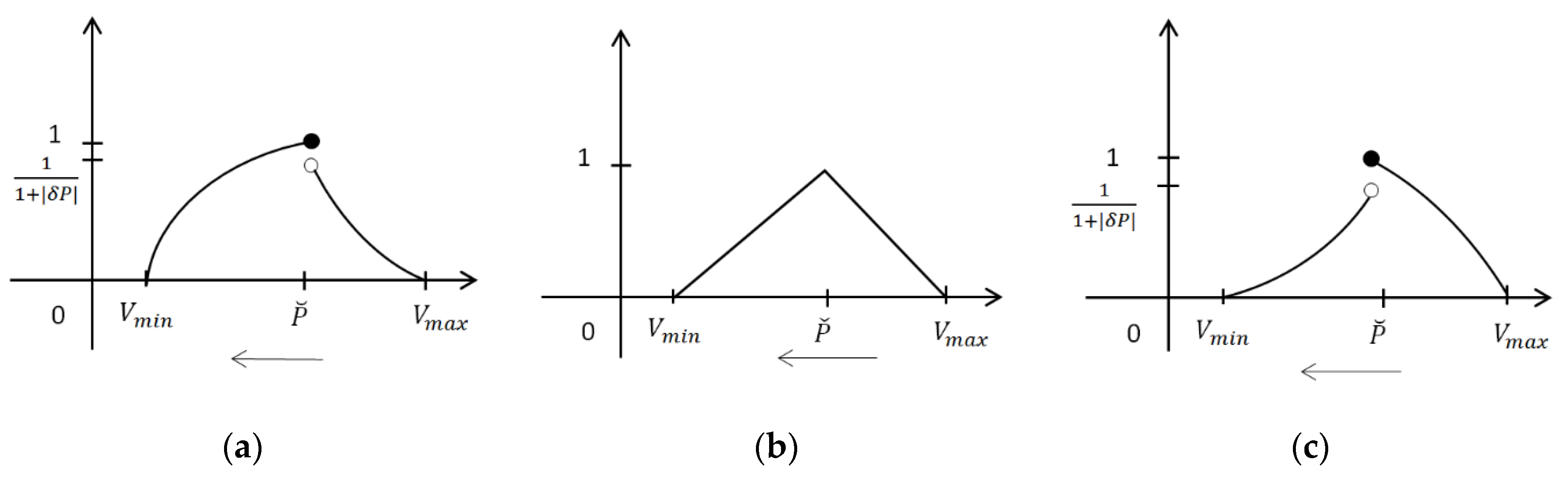
which approximates the quoted price $\check{P}$. F-BPV is described by its membership function ${\mu }_{BPV}$ determined separately for undervalued assets fulfilling the condition (30), fully valued assets fulfilling the condition (32), and overvalued assets fulfilling the condition (31). Figure 1a–c shows a graph of these membership functions.

Example 2.

In Example 1, we have evaluated the asset$\mathcal{Y}$by means of I-BPV. This asset is represented by the parameters vector$\mathbf{𝓿}=\left(60\$,30\$,30\$,80\$\right)$. Now, using (28–30) we evaluate an asset$\mathcal{Y}$by F-BPV equal to FN

$$\widetilde{BPV}\left(\mathbf{𝓿}\right)=ℒ\left(30,60,60,80, h\left(·|\mathbf{𝓿}\right),k\left(·|\mathbf{𝓿}\right)\right),$$

(50)

where

$$h\left(x|\mathbf{𝓿}\right)=\frac{4x-120}{x+60}\mathrm{for} x\in \left[30, 60\right[,$$

(51)

$$k\left(x|\mathbf{𝓿}\right)=\frac{3x-240}{x-140} \mathrm{for} x\in \left]60,80\right].$$

(52)

In line with (48), the membership function ${\mu }_{BPV}\left(·|\mathbf{𝓿}\right)\in {\left[0,1\right]}^{ℝ}$ F-BPV is given in following way:

$${\mu }_{BPV}\left(x|\mathbf{𝓿}\right)=\{\begin{array}{c} 0 , x\notin \left[30, 80\right],\\ \frac{4x-120}{x+60}, x\in \left[30,60\right[, \\ 1, x\in \left[60,60\right], \\ \frac{3x-240}{x-140}, x\in \left]60,80\right]. \end{array}$$

(53)

We see that F-BPV is fuzzy extension of PV model proposed by Rotschedla et al. [102].

8. Behavioural Present Value Represented by Oriented Fuzzy Numbers

Let us give the fixed parameter vector $\mathbf{𝓿}=\left(\check{P},P_0,V_{min},V_{max}\right)$ representing evaluated asset. In the previous chapter, we have considered its F-BPV represented by FN (46). The behavioural nature of investors is discussed in [133]. Among other things, this discussion shows that investors are also guided by their subjective predictions of quoted price closest changes. If we take into account these predictions, then we substitute F-BPV by oriented BPV (O-BPV) given as OFN

$$\overleftrightarrow{BPV}=\overleftrightarrow{ℒ}\left(V_s,\check{P}, \check{P},V_e, S_{BPV},E_{BPV}\right),$$

(54)

where

$$\left[V_s,V_e\right]\in \left\{\left[V_{min},V_{max}\right],\left[V_{max},V_{min}\right]\right\}$$

(55)

is the interval of all PPV,

$$S_{BPV}\left(x\right)=\{\begin{array}{c}h\left(x|\mathbf{𝓿}\right) V_s<V_e,\\ k\left(x|\mathbf{𝓿}\right) V_s>V_e,\end{array}$$

(56)

$$E_{BPV}\left(x\right)=\{\begin{array}{c}k\left(x|\mathbf{𝓿}\right) V_s<V_e,\\ h\left(x|\mathbf{𝓿}\right) V_s>V_e.\end{array}$$

(57)

The membership function ${\mu }_{BPV}\left(·|\mathbf{𝓿}\right)$ of OFN $\overleftrightarrow{BPV}\left(\mathbf{𝓿}\right)$ is given by the identity (46).

Positive O-BPV orientation predicts a rise in assets price. Then, O-BPV is given by the formula

$$\overleftrightarrow{BPV}\left(\mathbf{𝓿}\right)=\overleftrightarrow{ℒ}\left(V_{min},\check{P}, \check{P},V_{max}, h\left(·|\mathbf{𝓿}\right),k\left(·|\mathbf{𝓿}\right)\right).$$

(58)

In this way, we obtain three cases of O-BPV predicting a rise in asset price: for overvalued assets, for fully valued assets and for undervalued assets. The membership functions of these O-BPV kinds are presented in Figure 2a–c.

Negative O-BPV orientation predicts a fall in asset price. Then, O-BPV is given by the formula

$$\overleftrightarrow{BPV}\left(\mathbf{𝓿}\right)=\overleftrightarrow{ℒ}\left(V_{max},\check{P}, \check{P},V_{min}, k\left(·|\mathbf{𝓿}\right),h\left(·|\mathbf{𝓿}\right)\right).$$

(59)

In this way, we obtain three cases of O-BPV predicting fall in asset price: for overvalued assets, for fully valued assets and for undervalued assets. The membership functions of these OBPV kinds are presented in Figure 3a–c.

Example 3.

Among other things, in Example 1 we show that asset$\mathcal{Y}$is overvalued. In Example 2, we evaluate asset$\mathcal{Y}$by means of F-BPV (50).

Andrew and Helen are two people whose subjective forecasts of the change of future prices differ. Contrary to the recommendations of the economic theory, Andrew believes that $\mathcal{Y}$ quotations will increase in the near future. Therefore, he evaluates the asset $\mathcal{Y}$ by O-BPV:

$$\overleftrightarrow{BPV}\left(\mathbf{𝓿}\right)=\overleftrightarrow{ℒ}\left(30,60, 60,80, h\left(·|\mathbf{𝓿}\right),k\left(·|\mathbf{𝓿}\right)\right),$$

(60)

where the functions $h\left(·|\mathbf{𝓿}\right)$ and $k\left(·|\mathbf{𝓿}\right)$ are given, respectively, by (51) and (52). The O-BPV (60) is positively oriented. Its membership function is determined by (53).

In line with the economic theory, Helen is sure that the $\mathcal{Y}$ quotations will decrease in the near future. Therefore, she evaluates the asset $\mathcal{Y}$ by O-BPV:

$$\overleftrightarrow{BPV}\left(\mathbf{𝓿}\right)=\overleftrightarrow{ℒ}\left(80,60, 60,30, k\left(·|\mathbf{𝓿}\right),h\left(·|\mathbf{𝓿}\right)\right).$$

(61)

The O-BPV (61) is negatively oriented. Its membership function is given by (53). Moreover, this membership function may be equivalently determined as follows:

$${\mu }_{BPV}\left(x|\mathbf{𝓿}\right)=\{\begin{array}{l} 0, x\notin \left[80, 30\right],\\ \frac{3x-240}{x-140}, x\in \left[80,60\right[, \\ 1, x\in \left[60,60\right], \\ \frac{4x-120}{x+60}, x\in \left]60,30\right]. \end{array}$$

(62)

Let us note that membership functions (53) and (62) have the same graphs.

Each membership function of F-BPV or O-BPV is represented by a graph called the shortly BPV graph. The main objective of the presentation in Figure 1, Figure 2 and Figure 3 is to show the similarities between BPV graphs dedicated to different kinds of assets related to the same vector $\left(P_0,P_{min},P_{max},\alpha \right)$. We see that these graphs are similar. In particular, for considered case, we have here

• all overvalued assets have identical BPV graphs,
• all fully valued assets have identical BPV graphs,
• all undervalued assets have identical BPV graphs.

Therefore, we can conclude that a BPV graph and a BPV orientation are independent characteristics of BPV.

If we change vector $\left(P_0,P_{min},P_{max},\alpha \right)$, then obtained BPV graphs will only differ from one another in volatility range and its intensity of convexity.

9. Oriented Expected Return Determined by Behavioural Present Value

In this section, we apply O-BPV to determining the return rate similarly as Japanese candles were used in [42]. We will consider the asset represented parameters vector $\mathbf{𝓿}=\left(\check{P},P_0,V_{min},V_{max}\right)$.

For given due date $t>0$, the considered asset is characterised by following values:

• Predicted FV $V_t$,
• Evaluated PV $V_0$.

The benefits from owning this asset are characterised with use of a simple return rate $r_t$ determined as follows:

$$r_t=\frac{V_t-V_0}{V_0}=\frac{V_t}{V_0}-1.$$

(63)

In [42], it is justified in detail that FV is a random variable ${\tilde{V}}_t:\mathsf{\Omega }\to {ℝ}^{+}$ where the symbol $\mathsf{\Omega }$ denotes a space of all elementary states $\omega$ of the financial market. In a conventional approach to a return rate estimation, an asset PV is equal to quoted price $\check{P}$. Then, the return rate is a random variable given in the following way:

$$r_t\left(\omega \right)=\frac{{\tilde{V}}_t\left(\omega \right)-\check{P}}{\check{P}}.$$

(64)

We define any risk as a possibility of negative effects of taken actions. Uncertainty risk results from the lack of knowledge about the future conditions of the activities undertaken. In a financial analysis, an uncertainty risk is usually described by the probability distribution of return rate (64). The expected value $\overline{r}$ of this distribution is called expected return rate. We can assume that expected return rate $\overline{r}$ exists. The mentioned probability distribution can always be described by its cumulative distribution function $F_r\left(·|\overline{r}\right):ℝ\to \left[0,1\right]$. From (64), we immediately get

$${\tilde{V}}_t\left(\omega \right)=\check{P}·\left(1+r_t\left(\omega \right)\right).$$

(65)

If we take together (63) and (65), then we obtain the following formula describing the return rate:

$$r_t=r_t\left(V_0,\omega \right)=\frac{\check{P}·\left(1+r_t\left(\omega \right)\right)}{V_0}-1.$$

(66)

It implies that the expected return rate is given by formula

$$ℛ\left(V_0\right)={{\displaystyle \int }}_{-\infty }^{+\infty }\frac{\check{P}·\left(1+y\right)}{V_0}-1d{F}_r\left(y|\overline{r}\right)=\frac{\check{P}·\left(1+\overline{r}\right)}{V_0}-1.$$

(67)

In this manner, we determine the expected return rate $ℛ:{ℝ}^{+}\to ℝ$ as a unary operator transforming PV. If PV is imprecisely estimated by O-PV, then using the Kosinski’s approach, we define the expected return rate by an extension $\overleftrightarrow{ℛ}:\mathbb{K}\to \mathbb{K}$ of a unary operator (67).

We consider now the case of O-PV equal to O-BPV $\overleftrightarrow{BPV}\left(\mathbf{𝓿}\right)$ given by (54). Its starting and ending functions are strictly monotonic. Therefore, the identities (21), (26), (27), and (67) imply that the expected return rate is given by an equation

$$\overleftrightarrow{ℒ}\left(\frac{\check{P}·\left(1+\overline{r}\right)}{V_s}-1,\overline{r},\overline{r},\frac{\check{P}·\left(1+\overline{r}\right)}{V_e}-1,S_R, E_R\right)=\overleftrightarrow{ℛ}\left(\overleftrightarrow{ℒ}\left(V_s,\check{P}, \check{P},V_e, S_{BPV},E_{BPV}\right)\right),$$

(68)

where

$${\forall }_{r\in \left[\frac{\check{P}·\left(1+\overline{r}\right)}{V_s}-1,\overline{r}\right[} : S_R\left(r\right)=S_{BPV}\left({ℛ}^{-1}\left(r\right)\right)=S_{BPV}\left(\check{P}·\frac{1+\overline{r}}{1+r}\right),$$

(69)

$${\forall }_{r\in \left]\overline{r},\frac{\check{P}·\left(1+\overline{r}\right)}{V_e}-1\right]} : E_R\left(r\right)=E_{BPV}\left({ℛ}^{-1}\left(r\right)\right)=E_{BPV}\left(\check{P}·\frac{1+\overline{r}}{1+r}\right),$$

(70)

where the interval $\left[V_s,V_e\right]$ is determined by (55). If we compare (69) and (70) with (56) and (57), then we get

$$S_R\left(r\right)=\{\begin{array}{c}h\left(\check{P}·\frac{1+\overline{r}}{1+r}|\mathbf{𝓿}\right), V_s<V_e,\\ k\left(\check{P}·\frac{1+\overline{r}}{1+r}|\mathbf{𝓿}\right), V_s>V_e,\end{array}$$

(71)

$$E_R\left(r\right)=\{\begin{array}{c}k\left(\check{P}·\frac{1+\overline{r}}{1+r}|\mathbf{𝓿}\right), V_s<V_e,\\ h\left(\check{P}·\frac{1+\overline{r}}{1+r}|\mathbf{𝓿}\right), V_s>V_e.\end{array}$$

(72)

The identities (54) and (68) show that O-BPV and the expected return rate determined by are it appositively oriented. Therefore, we can say the following.

• If O-BPV describes a subjective belief about rise in quotations, then we can anticipate a decline in the expected return rate.
• If O-BPV describes a subjective belief about fall in quotations, then we can anticipate an upturn in the expected return rate.

In finance, both of above facts are well known. This observation proves that the extension of F-PV model to the case of O-PV model is an appropriate direction for the development of fuzzy finance theory.

Example 4.

The asset$\mathcal{Y}$is overvalued. Despite this, Andrew believes that$\mathcal{Y}$quotations will increase in the near future. Therefore, he evaluates the asset$\mathcal{Y}$by positively oriented O-BPV (60). On the other hand, the$\mathcal{Y}$quotations are characterised by an expected quarterly return rate$\overline{r}=0.02$. If Andrew determines the expected return rate$\overleftrightarrow{ℛ}$with use O-BPV, then he gets

$$\overleftrightarrow{ℛ}=\overleftrightarrow{ℒ}\left(1.04, 0.02, 0.02,-0.235,S_R, E_R\right)$$

(73)

where

$$S_R\left(r\right)=\frac{124.8-120·r}{121.2+60·r},$$

(74)

$$E_R\left(r\right)=\frac{56.4+240·r}{201.2+140·r}.$$

(75)

We see that expected return is negatively oriented. Moreover, Andrew shows that membership function of the expected return rate $\overleftrightarrow{ℛ}$ is given as follows

$$\rho \left(r|\mathbf{𝓿}\right)={\mu }_{BPV}\left(\frac{61.2}{1+r}|\mathbf{𝓿}\right)=\{\begin{array}{c}0, r\notin \left[1.04, -0.235\right],\\ \frac{124.8-120·r}{121.2+60·r}, r\in \left[1.04, 0.02\right[, \\ 1, r\in \left[0.02, 0.02\right], \\ \frac{56.4+240·r}{201.2+140·r}, r\in \left]0.02, -0.235\right]. \end{array}$$

(76)

10. Conclusions

Apart from the theory of interest, any PV is an ambiguous value determined under the influence of, among others, behavioural premises. This view was fully substantiated by the literature study presented in Section 2. This sufficiently proves the need to use soft computing techniques for PV evaluation.

For this reason, in Section 5, BPV is generally defined as the set of all real numbers equal to possible PVs. It is obvious that BPV is an imprecise number. In this paper, we discuss BPV approximation given as following kinds of imprecision numbers:

• I-BPV approximated by interval numbers in Section 6,
• F-BPV approximated by FNs in Section 7,
• O-BPV approximated by OFNs in Section 8.

Interval numbers are definitely a poorer form of information than FNs. For this reason, we should always replace I-BPV with F-BPV. This replacement does not require any additional data. In [126], it is shown that oriented PV application for a portfolio analysis is more useful than the analogous application of fuzzy PV. This makes the use of O-BPV more preferred than the use of F-BPV.

Each of the proposed BPV models is determined by a specific membership function. We are of the opinion that each of the above-mentioned models can be described by means of different membership functions. The search for new membership function proposals may be very fruitful direction for further research.

In [134,135], it is shown that BPV may be valued by intuitionistic FNs [136]. We believe that other types of imprecise numbers can also be used as BPV models. Looking for such opportunities is an interesting direction for further research. However, we must remember that each proposed modelling method for BPV should be carefully justified by serious financial or behavioural reasons. Proposing new BPV models, researchers should also remember about the results contained in [137].

Section 9 describes in detail an application of O-BPV for determining return rate. This result facilitates the use of O-BPV for an analysis of assets with PV estimated by OFN. It is expedient to further develop the fuzzy finance theory based on OFN. On the other hand, the O-BPV may be applied in such algorithms based on financial technical analysis which support invest-making. For example, here we can apply the advice-making algorithms described in [61,62]. Moreover, we can use O-BPV as input signal to fuzzy or neuro-fuzzy systems explained in detail in [138]. The assessment of the suitability of BPV to support decisions is an interesting direction for further research.

References

- Piasecki, K. Basis of Financial Arithmetic from the Viewpoint of the Utility Theory. Oper. Res. Decis. 2012, 22, 37–53. [Google Scholar]
- Dubois, D.; Prade, H. Operations on Fuzzy Numbers. Int. J. Syst. Sci. 1978, 9, 613–629. [Google Scholar] [CrossRef]
- Ward, T.L. Discounted Fuzzy Cash Flow Analysis. Fall Ind. Eng. Conf. Proc. 1985, 476, 481. [Google Scholar]
- Buckley, J.J. The Fuzzy Mathematics of Finance. Fuzzy Sets Syst. 1987, 21, 257–273. [Google Scholar] [CrossRef]
- Greenhut, J.G.; Norman, G.; Temponi, C.T. Towards a Fuzzy Theory of Oligopolistic Competition. In Proceedings of the 3rd International Symposium on Uncertainty Modeling and Analysis and Annual Conference of the North American Fuzzy Information Processing Society, College Park, MD, USA, 17–20 September 1995; IEEE: College Park, MD, USA; pp. 286–291. [Google Scholar]
- Sheen, J.N. Fuzzy Financial Profitability Analyses of Demand Side Management Alternatives from Participant Perspective. Inf. Sci. 2005, 169, 329–364. [Google Scholar] [CrossRef]
- Gutierez, I. Fuzzy Numbers and Net Present Value. Scand. J. Mgmt. 1989, 5, 149–159. [Google Scholar] [CrossRef]
- Kuchta, D. Fuzzy Capital Budgeting. Fuzzy Sets Syst. 2000, 111, 367–385. [Google Scholar] [CrossRef]
- Lesage, C. Discounted Cash-flows Analysis. An Interactive Fuzzy Arithmetic Approach. Eur. J. Econ. Soc. Syst. 2001, 15, 49–68. [Google Scholar] [CrossRef] [Green Version]
- Huang, X. Two New Models for Portfolio Selection with Stochastic Returns Taking Fuzzy Information. Eur. J. Oper. Res. 2007, 180, 396–405. [Google Scholar] [CrossRef]
- Tsao, C.T. Assessing the Probabilistic Fuzzy Net Present Value for a Capital, Investment Choice Using Fuzzy Arithmetic. J. Chin. Ins. Ind. Eng. 2005, 22, 106–118. [Google Scholar] [CrossRef]
- Calzi, M.L. Towards a General Setting for the Fuzzy Mathematics of Finance. Fuzzy Sets Syst. 1990, 35, 265–280. [Google Scholar] [CrossRef]
- Piasecki, K. Behavioural Present Value. SSRN Electron. J. 2011, 1, 1–17. [Google Scholar] [CrossRef] [Green Version]
- Baerecke, T.; Bouchon-Meunier, B.; Detyniecki, M. Fuzzy Present Value. In Proceedings of the 2011 IEEE Computational Intelligence for Financial Engineering and Economics, Paris, France, 11–15 April 2011; IEEE Symposium: Paris, France, 2011; pp. 1–6. [Google Scholar]
- Biswas, P.; Pramanik, S. Fuzzy Approach to Replacement Problem with Value of Money Changes with Time. Int. J. Comput. Appl. 2011, 30, 28–33. [Google Scholar] [CrossRef]
- Nosratpour, M.; Nazeri, A.; Meftahi, H. Fuzzy Net Present Value for Engineering Analysis. Manag. Sci. Lett. 2012, 2, 2153–2158. [Google Scholar] [CrossRef]
- Piasecki, K. Effectiveness of Securities with Fuzzy Probabilistic Return. Oper. Res. Decis. 2011, 21, 65–78. [Google Scholar]
- Piasecki, K. On Imprecise Investment Recommendations. Stud. Log. Gramm. Rhetor. 2014, 37, 179–194. [Google Scholar] [CrossRef] [Green Version]
- Li, X.; Quin, Z.; Kar, S. Mean-Variance-Skewness Model for Portfolio Selection with Fuzzy Returns. Eur. J. Oper. Res. 2010, 202, 239–247. [Google Scholar] [CrossRef]
- Quin, Z.; Wen, M.; Gu, C. Mean-absolute Deviation Portfolio Selection Model with Fuzzy Returns. Iran. J. Fuzzy Syst. 2011, 8, 61–75. [Google Scholar]
- Tsaur, R. Fuzzy Portfolio Model with Different Investor Risk Attitudes. Eur. J. Oper. Res. 2013, 227, 385–390. [Google Scholar] [CrossRef]
- Tanaka, H.; Guo, P.; Turksen, B. Portfolio Selection Based on Fuzzy Probabilities and Possibility Distributions. Fuzzy Sets Syst. 2000, 111, 387–397. [Google Scholar] [CrossRef]
- Duan, L.; Stahlecker, P. A Portfolio Selection Model Using Fuzzy Returns. Fuzzy Optim. Decis. Mak. 2011, 10, 167–191. [Google Scholar] [CrossRef]
- Guo, H.; Sun, B.; Karimi, H.R.; Ge, Y.; Jin, W. Fuzzy Investment Portfolio Selection Models Based on Interval Analysis Approach. Math. Probl. Eng. 2012. [Google Scholar] [CrossRef]
- Gupta, P.; Mittal, G.; Mehlawat, M.K. Multiobjective Expected Value Model for Portfolio Selection in Fuzzy Environment. Optim. Lett. 2013, 7, 1765–1791. [Google Scholar] [CrossRef]
- Gupta, P.; Mittal, G.; Saxena, A. Asset Portfolio Optimization Using Fuzzy Mathematical Programming. Inf. Sci. 2008, 178, 1734–1755. [Google Scholar] [CrossRef]
- Huang, X.; Shen, W. Multi-period Mean-variance Model with Transaction Cost for Fuzzy Portfolio Selection. In Proceedings of the Seventh International Conference on Fuzzy Systems and Knowledge Discovery, Yantai, Shandong, China, 10–12 August 2010. [Google Scholar] [CrossRef]
- Liu, Y.; Sun, L. Comparative Research of Portfolio Model Using Fuzzy Theory. In Proceedings of the Fourth International Conference on Fuzzy Systems and Knowledge Discovery, Haikou, China, 24–27 August 2007. [Google Scholar] [CrossRef]
- Liu, Y.J.; Zhang, W.G. Fuzzy Portfolio Optimization Model Under Real Constraints. Insur. Math. Econ. 2013, 53, 704–711. [Google Scholar] [CrossRef]
- Wu, X.L.; Liu, Y.K. Optimizing Fuzzy Portfolio Selection Problems by Parametric Quadratic Programming. Fuzzy Optim. Decis. Mak. 2012, 11, 411–449. [Google Scholar] [CrossRef]
- Wang, S.; Zhu, S. On Fuzzy Portfolio Selection Problems. Fuzzy Optim. Decis. Mak. 2002, 1, 361–377. [Google Scholar] [CrossRef]
- Mehlawat, M.K. Credibilistic Mean-entropy Models for Multi-period Portfolio Selection with Multi-choice Aspiration Levels. Inf. Sci. 2016, 345, 9–26. [Google Scholar] [CrossRef]
- Kahraman, C.; Ruan, D.; Tolga, E. Capital Budgeting Techniques Using Discounted Fuzzy Versus Probabilistic Cash Flows. Inf. Sci. 2002, 142, 57–76. [Google Scholar] [CrossRef]
- Fang, Y.; Lai, K.K.; Wang, S. Fuzzy Portfolio Optimization. Theory and Methods. In Lecture Notes in Economics and Mathematical Systems; Springer: Berlin, Germany, 2008; Volume 609. [Google Scholar]
- Gupta, P.; Mehlawat, M.K.; Inuiguchi, M.; Chandra, S. Fuzzy Portfolio Optimization. Advances in Hybrid Multi-criteria Methodologies. In Studies in Fuzziness and Soft Computing; Springer: Berlin, Germany, 2014; Volume 316. [Google Scholar] [CrossRef]
- Kosiński, W.; Prokopowicz, P.; Ślęzak, D. Fuzzy Numbers with Algebraic Operations: Algorithmic Approach. In Proceedings of the Eight International Conference on Information, Logistics & Supply Chain–ILS 2020, Austin, TX, USA, 22–24 April 2020; Klopotek, M., Wierzchoń, S.T., Michalewicz, M., Eds.; Physica Verlag: Sopot, Poland; Springer: Berlin/Heidelberg, Germany, 2002; pp. 311–320. [Google Scholar]
- Kosiński, W. On Fuzzy Number Calculus. Int. J. Appl. Math. Comput. Sci. 2006, 16, 51–57. [Google Scholar]
- Piasecki, K. Revision of the Kosiński’s Theory of Ordered Fuzzy Numbers. Axioms 2018, 7, 16. [Google Scholar] [CrossRef] [Green Version]
- Prokopowicz, P. The Directed Inference for the Kosinski’s Fuzzy Number Model. In Proceedings of the Second International Afro-European Conference for Industrial Advancement, Villejuif, France, 9–11 September 2015. [Google Scholar]
- Prokopowicz, P.; Pedrycz, W. The Directed Compatibility Between Ordered Fuzzy Numbers—A Base Tool for a Direction Sensitive Fuzzy Information Processing. In Advances in Inteligent Systems and Computing; Abraham, A., Wegrzyn-Wolska, K., Hassanien, A.E., Snasel, V., Alimi, A.M., Eds.; Springer: Cham, Switzerland, 2015; Volume 127, pp. 493–505. [Google Scholar] [CrossRef]
- Prokopowicz, P.; Pedrycz, W. The Directed Compatibility between Ordered Fuzzy Numbers–A Base Tool for a Direction Sensitive Fuzzy Information Processing. In Proceedings of the Artificial Intelligence and Soft Computing ICAISC 2015, Lecture Notes in Computer Science. Zakopane, Poland, 14–18 June 2015; Rutkowski, L., Korytkowski, M., Scherer, R., Tadeusiewicz, R., Zadeh, L., Zurada, J., Eds.; Springer: Cham, Switzeland, 2015; Volume 9119. [Google Scholar] [CrossRef]
- Piasecki, K. Relation “Greater Than or Equal to” Between Ordered Fuzzy Numbers. Appl. Syst. Innov. 2019, 2, 26. [Google Scholar] [CrossRef] [Green Version]
- Piasecki, K.; Łyczkowska-Hanćkowiak, A. Representation of Japanese Candlesticks by Oriented Fuzzy Numbers. Economics 2020, 8, 1. [Google Scholar] [CrossRef] [Green Version]
- Prokopowicz, P.; Czerniak, J.; Mikołajewski, D.; Apiecionek, Ł.; Ślȩzak, D. Analysis of Temporospatial Gait Parameters. In Theory and Applications of Ordered Fuzzy Number; Springer: Berlin, Germany, 2017; Volume 356, pp. 289–302. [Google Scholar]
- Kacprzak, D.; Kosiński, W.; Kosiński, W.K. Financial Stock Data and Ordered Fuzzy Numbers. In Proceedings of the Artificial Intelligence and Soft Computing. ICAISC 2013, Zakopane, Poland, 9–13 June 2013; Lecture Notes in Computer Science. Springer: Berlin/Heidelberg, Germany, 2013; Volume 7894, pp. 259–270. [Google Scholar]
- Kacprzak, D.; Kosiński, W. Optimizing Firm Inventory Costs as a Fuzzy Problem. Stud. Log. Gramm. Rhetor. 2014, 37, 89–105. [Google Scholar] [CrossRef] [Green Version]
- Chwastyk, A.; Pisz, I. OFN Capital Budgeting Under Uncertainty and Risk. In Theory and Applications of Ordered Fuzzy Number; Prokopowicz, P., Czerniak, J., Mikołajewski, D., Apiecionek, Ł., Ślȩzak, D., Eds.; Springer: Berlin, Germany, 2017; Volume 356, pp. 157–170. [Google Scholar]
- Czerniak, J.M. OFN Ant Method Based on TSP Ant Colony Optimization. In Theory and Applications of Ordered Fuzzy Number; Prokopowicz, P., Czerniak, J., Mikołajewski, D., Apiecionek, Ł., Ślȩzak, D., Eds.; Springer: Berlin, Germany, 2017; Volume 356, pp. 207–222. [Google Scholar]
- Ewald, D.; Czerniak, J.M.; Paprzycki, M. A New OFN Bee Method as an Example of Fuzzy Observance Applied for ABC Optimization. In Theory and Applications of Ordered Fuzzy Number; Prokopowicz, P., Czerniak, J., Mikołajewski, D., Apiecionek, Ł., Ślȩzak, D., Eds.; Springer: Berlin, Germany, 2017; Volume 356, pp. 223–238. [Google Scholar]
- Kacprzak, D. Input-Output Model Based on Ordered Fuzzy Numbers. In Theory and Applications of Ordered Fuzzy Number; Prokopowicz, P., Czerniak, J., Mikołajewski, D., Apiecionek, Ł., Ślȩzak, D., Eds.; Springer: Berlin, Germany, 2017; Volume 356, pp. 171–182. [Google Scholar]
- Kacprzak, D. Objective Weights Based on Ordered Fuzzy Numbers for Fuzzy Multiple Criteria Decision-making Methods. Entropy 2017, 19, 373. [Google Scholar] [CrossRef] [Green Version]
- Marszałek, A.; Burczyński, T. Ordered fuzzy candlesticks. In Theory and Applications of Ordered Fuzzy Number; Prokopowicz, P., Czerniak, J., Mikołajewski, D., Apiecionek, Ł., Ślȩzak, D., Eds.; Springer: Berlin, Germany, 2017; Volume 356, pp. 183–194. [Google Scholar] [CrossRef]
- Piasecki, K. Expected Return Rate Determined as Oriented Fuzzy Number. In Proceedings of the 35th International Conference Mathematical Methods in Economics Conference, Hradec Králové, Czech Republic, 13–15 September 2017; pp. 561–565. [Google Scholar]
- Roszkowska, E.; Kacprzak, D. The Fuzzy SAW and Fuzzy TOPSIS Procedures Based on Ordered Fuzzy Numbers. Inf. Sci. 2016, 369, 564–584. [Google Scholar] [CrossRef]
- Rudnik, K.; Kacprzak, D. Fuzzy TOPSIS Method with Ordered Fuzzy Numbers for Flow Control in a Manufacturing System. Appl. Soft Comput. 2017, 52, 1020–1041. [Google Scholar] [CrossRef]
- Zarzycki, H.; Czerniak, J.M.; Dobrosielski, W.T. Detecting Nasdaq Composite Index Trends with OFNs. In Theory and Applications of Ordered Fuzzy Number; Prokopowicz, P., Czerniak, J., Mikołajewski, D., Apiecionek, Ł., Ślȩzak, D., Eds.; Springer: Berlin, Germany, 2017; Volume 356, pp. 195–206. [Google Scholar]
- Łyczkowska-Hanćkowiak, A.; Piasecki, K. Two-assets Portfolio with Trapezoidal Oriented Fuzzy Present values. In Proceedings of the 36th International Conference Mathematical Methods in Economics Conference, Jindřichův Hradec, Czech Republic, 12–14 September 2018; pp. 306–311. [Google Scholar]
- Łyczkowska-Hanćkowiak, A.; Piasecki, K. Present Value of Portfolio of Assets with Present Values Determined by Trapezoidal Ordered Fuzzy Numbers. Oper. Res. Decis. 2018, 28, 41–56. [Google Scholar]
- Piasecki, K.; Roszkowska, E. On Application of Ordered Fuzzy Numbers in Ranking Linguistically Evaluated Negotiation Offers. Adv. Fuzzy Syst. 2018. [Google Scholar] [CrossRef]
- Piasecki, K.; Roszkowska, E.; Łyczkowska-Hanćkowiak, A. Simple Additive Weighting Method Equipped with Fuzzy Ranking of Evaluated Alternatives. Symmetry 2019, 11, 482. [Google Scholar] [CrossRef] [Green Version]
- Piasecki, K.; Roszkowska, E.; Łyczkowska-Hanćkowiak, A. Impact of the Orientation of the Ordered Fuzzy Assessment on the Simple Additive Weighted Method. Symmetry 2019, 11, 1104. [Google Scholar] [CrossRef] [Green Version]
- Łyczkowska-Hanćkowiak, A. Sharpe’s Ratio for Oriented Fuzzy Discount Factor. Mathematics 2019, 7, 272. [Google Scholar] [CrossRef] [Green Version]
- Łyczkowska-Hanćkowiak, A. On Application Oriented Fuzzy Numbers for Imprecise Investment Recommendations. Symmetry 2020, 12, 1672. [Google Scholar] [CrossRef]
- Piasecki, K.; Siwek, J. Behavioural Present Value Defined as Fuzzy Number a New Approach. Folia Oeconomica Stetin. 2015, 15, 27–41. [Google Scholar] [CrossRef] [Green Version]
- Łyczkowska-Hanćkowiak, A. Behavioural Present Value Determined by Ordered Fuzzy Number. SSRN Electron. J. 2017. [Google Scholar] [CrossRef]
- Peccati, L. Su di Una Caratterizzazione del Principio del Criterio Dell’attualizzazione. In Studium Parmense; Università di Parma: Parma, Italy, 1972. [Google Scholar]
- Janssen, J.; Manca, R.; Volpe di Prignano, E. Mathematical Finance. Deterministic and Stochastic Models; John Wiley & Sons: London, UK, 2009. [Google Scholar]
- Ramsey, F.P.A. Mathematical Theory of Saving. Econ. J. 1928, 38, 543–559. [Google Scholar] [CrossRef]
- Samuelson, P.A. A Note on Measurement of Utility. Rev. Econ. Stud. 1937, 4, 155–161. [Google Scholar] [CrossRef]
- Koopmans, T.C.; Diamond, P.A.; Williamson, R.E. Stationary Utility and Time Perspective. Econom. J. Econom. Soc. 1964, 32, 82–100. [Google Scholar] [CrossRef]
- Strotz, R.H. Myopia and Inconsistency in Dynamic Utility Maximization. Rev. Econ. Stud. 1955, 23. [Google Scholar] [CrossRef]
- Loewenstein, G.; Prelec, D. Anomalies in Intertemporal Choice: Evidence and Interpretation. Q. J. Econ. 1992, 107, 573–597. [Google Scholar] [CrossRef]
- Frederick, S.; Loewenstein, G.; O’Donoghue, T. Time Discounting and Time Preference: A Critical Review. J. Econ. Lit. 2002, 40, 351–401. [Google Scholar] [CrossRef]
- Streich, P.; Levy, J.S. Time Horizons, Discounting, and Intertemporal Choice. J. Confl. Resolut. 2007, 51, 199–226. [Google Scholar] [CrossRef] [Green Version]
- Thaler, R.H. Some Empirical Evidence on Dynamic Inconsistency. Econ. Lett. 1981, 8. [Google Scholar] [CrossRef]
- Herrnstein, R.J. Rational Choice Theory: Necessary but not Sufficient. Am. Psychol. 1990, 45. [Google Scholar] [CrossRef]
- Mazur, J.E. An Adjusting Procedure for Studying Delayed Reinforcement. In The Effect of Delay and of Intervening Events on Reinforcement Value. Quantitative Analysis of Behavior; Commons, M.L., Mazur, J.E., Nevin, J.A., Rachlin, H., Eds.; Lawrence Erlbaum Associates, Inc.: Mahwah, NJ, USA, 1987; pp. 55–73. [Google Scholar]
- Ainslie, G. Specious Reward: A Behavioral Theory of Impulsiveness and Impulse Control. Psychol. Bull. 1975, 82. [Google Scholar] [CrossRef] [Green Version]
- Herrnstein, R.J. Self-control as Response Strength. In Quantification of Steady-state Operant Behavior; Elsevier/North Holland Biomedical Press: Amsterdam, The Netherlands, 1981. [Google Scholar]
- Doyle, J.R. Survey of Time Preference, Delay Discounting Model. Judgm. Decis. Mak. 2013, 8, 116–135. [Google Scholar] [CrossRef] [Green Version]
- Killeen, P.R. An Additive-utility Model of Delay Discounting. Psychol. Rev. 2009, 116, 602–619. [Google Scholar] [CrossRef] [PubMed]
- Rachlin, H. Notes on Discounting. J. Exp. Anal. Behav. 2006, 85, 425–435. [Google Scholar] [CrossRef] [Green Version]
- Laibson, D. Golden Eggs and Hyperbolic Discounting. Q. J. Econ. 1997, 112, 443–477. [Google Scholar] [CrossRef] [Green Version]
- Benhabib, J.; Bisin, A.; Schotter, A. Present Bias, Quasi-hyperbolic Discounting, and Fixed Costs. Games Econ. Behav. 2010, 69, 205–223. [Google Scholar] [CrossRef]
- Commons, M.L. How Reinforcement Density is Discriminated and Scaled. In Quantitative Analyses of Behavior. Discriminative Properties of Reinforcement Schedules; Commons, M.L., Nevin, J.A., Eds.; Ballinger: Cambridge, MA, USA, 1981; Volume 1. [Google Scholar]
- Commons, M.L.; Woodford, M.; Ducheny, J.R. The Relationship Between Perceived Density of Reinforcement in a Schedule Sample Audits Reinforcing Value. In Quantitative Analysis of Behavior. Matching and Maximizing Accounts; Commons, M.L., Nevin, J.A., Eds.; Ballinger: Cambridge, MA, USA, 1982; Volume 2. [Google Scholar]
- Davison, M.C. Preference for Mixed-interval Versus Fixed-interval Schedules. J. Exp. Anal. Behav. 1969, 12, 247–252. [Google Scholar] [CrossRef] [Green Version]
- Du, W.; Green, L.; Myerson, J. Cross-cultural Comparisons of Discounting Delayed and Probabilistic Rewards. Psychol. Rec. 2002, 52, 479–492. [Google Scholar] [CrossRef]
- Roelofsma, P.H.M.P. Modeling Intertemporal Choices: An Anomaly Approach. Acta Psychol. 1996, 93, 5–22. [Google Scholar] [CrossRef]
- Ebert, J.E.; Prelec, D. The Fragility of Time: Time-insensitivity and Valuation of the Near and Future. Manag. Sci. 2007, 53, 1423–1438. [Google Scholar] [CrossRef] [Green Version]
- Myerson, J.; Green, L. Discounting of Delayed Rewards: Models of Individual Choice. J. Exp. Anal. Behav. 1995, 64, 263–276. [Google Scholar] [CrossRef] [PubMed] [Green Version]
- Read, D. Is time Discounting Hyperbolic or Subadditive? J. Risk Uncertain. 2001, 23, 5–32. [Google Scholar] [CrossRef]
- Masin, S.C.; Zudini, V.; Antonelli, M. Early Alternative Derivations of Fechner’s Law. J. Hist. Behav. Sci. 2009, 45, 56–65. [Google Scholar] [CrossRef] [PubMed]
- Bleichrodt, H.; Rohde, K.I.M.; Wakker, P.P. Non-hyperbolic Time Inconsistency. Games Econ. Behav. 2009, 66, 27–38. [Google Scholar] [CrossRef]
- Stevens, S.S. On the Psychophysical Law. Psychol. Rev. 1957, 64, 153–181. [Google Scholar] [CrossRef]
- Stevens, S.S. To Honor Fechner and Repeal His Law. Science 1961, 133, 80–86. [Google Scholar] [CrossRef] [PubMed]
- Piasecki, K. Discounting Under Impact of Temporal Risk Aversion—A Case of Discrete Time. Res. Pap. Wrocław Univ. Econ. 2015, 381, 289–298. [Google Scholar] [CrossRef]
- Piasecki, K. Discounting Under Impact of Temporal Risk Aversion—A Case of Continuous Time. In Economic Development and Management of Regions; Jedlička, P., Ed.; Gaudeamus, University of Hradec Kralove: Hradec Králové, Chezh Republic, 2015; Volume 5. [Google Scholar]
- Piasecki, K. Discounting Under Impact of Risk Aversion. SSRN Electron. J. 2015. [Google Scholar] [CrossRef]
- Ok, E.A.; Masatlioglu, Y. A Theory of (Relative) Discounting. J. Econ. Theory 2007, 137, 214–245. [Google Scholar] [CrossRef]
- Dubra, J. A Theory of Time Preferences Over Risky Outcomes. J. Math. Econ. 2009, 45, 576–588. [Google Scholar] [CrossRef] [Green Version]
- Rotschedl, J.; Kaderabkova, B.; Čermáková, K. Parametric Discounting Model of Utility. Procedia Econ. Financ. 2015, 30, 730–741. [Google Scholar] [CrossRef] [Green Version]
- Von Mises, L. The Ultimate Foundation of Economic Science. An Essay on Method; D. Van Nostrand Company, Inc.: Princeton, NJ, USA, 1962. [Google Scholar]
- Tversky, A.; Kahneman, D. Availability: A Heuristic for Judging Frequency and Probability. Cogn. Psychol. 1973, 5, 207–232. [Google Scholar] [CrossRef]
- Tversky, A.; Kahneman, D. Judgment Under Uncertainty: Heuristic and Biases. Science 1974, 185, 1124–1131. [Google Scholar] [CrossRef]
- Barberis, N.; Shleifer, A.; Vishny, R. A Model of Investor Sentiment. J. Financ. Econ. 1998, 49, 307–343. [Google Scholar] [CrossRef]
- Daniel, K.; Hirshleifer, D.; Subrahmanyam, A. Overconfidence, Arbitrage and Equilibrium Asset Pricing. J. Financ. 2001, 56, 921–965. [Google Scholar] [CrossRef]
- Hong, H.; Stein, J. A Unified Theory of Under Reaction, Momentum Trading and Over Reaction in Asset Market. J. Financ. 1999, 54, 2143–2184. [Google Scholar] [CrossRef] [Green Version]
- Ainslie, G.; Haendel, V. The Motives of the Will. In Etiologic Aspects of Alcohol and Drug Abuse, Springfield; Gottheil, E., Druley, K.A., Skoloda, T.E., Waxman, H., Eds.; Charles, C. Thomas: Springfield, IL, USA, 1983; pp. 119–140. [Google Scholar]
- Kirby, K.N. Bidding on the Future: Evidence Against Normative Discounting of Delayed Rewards. J. Exp. Psychol. Gen. 1997, 126, 54–70. [Google Scholar] [CrossRef]
- Kirby, K.N.; Marakovič, N.N. Modeling Myopic Decision: Evidence for Hyperbolic Delay-Discounting with Subjects and Amounts. Organ. Behav. Hum. Decis. Process. 1995, 64, 22–30. [Google Scholar] [CrossRef]
- Kahneman, D.; Tversky, A. Prospect Theory: An Analysis of Decision under Risk. Econometica 1979, 47, 263–292. [Google Scholar] [CrossRef] [Green Version]
- Loewenstein, G. Frames of Mind in Intertemporal Choice. Manag. Sci. 1988, 34, 200–214. [Google Scholar] [CrossRef] [Green Version]
- Shelley, M.K. Outcome Signs, Question Frames and Discount Rates. Manag. Sci. 1993, 39, 806–815. [Google Scholar] [CrossRef] [Green Version]
- Kirby, K.N.; Santiesteban, M. Concave Utility, Transaction Costs and Risk in Measuring Discounting of Delayed Rewards. J. Exp. Psychol. Learn. Mem. Cogn. 2003, 29, 66–79. [Google Scholar] [CrossRef]
- Fishburn, P.; Edwards, W. Discount Neutral Utility Models for Denumerable Time Streams. Theory Decis. 1997, 43, 139–166. [Google Scholar] [CrossRef]
- Dacey, R.; Zielonka, P. A Detailed Prospect Theory Explanation of the Disposition Effect. J. Behav. Financ. 2008, 9, 43–50. [Google Scholar] [CrossRef]
- Zauberman, G.; Kyu Kim, B.; Malkoc, S.; Bettman, J.R. Discounting Time and Time Discounting: Subjective Time Perception and Intertemporal Preferences. J. Mark. Res. 2009, 46, 543–556. [Google Scholar] [CrossRef]
- Kim, B.K.; Zauberman, G. Perception of Anticipatory Time in Temporal Discounting. J. Neurosci. Psychol. Econ. 2009, 2, 91–101. [Google Scholar] [CrossRef] [Green Version]
- Epper, T.; Fehr-Duda, H.; Bruhin, A. Uncertainty Breeds Decreasing Impatience: The Role of Risk Preferences in Time Discounting. SSRN Electron. J. 2009, 412. [Google Scholar] [CrossRef] [Green Version]
- Kontek, K. Decision Utility Theory: Back to von Neumann, Morgenstern, and Markowitz. SSRN Electron. J. 2009. [Google Scholar] [CrossRef] [Green Version]
- Rabin, M. Incorporating Fairness into Game Theory and Economics. Am. Econ. Rev. 1993, 83, 1281–1302. [Google Scholar]
- Delgado, M.; Vila, M.A.; Voxman, W. On a Canonical Representation of Fuzzy Numbers. Fuzzy Sets Syst. 1998, 93, 125–135. [Google Scholar] [CrossRef]
- Goetschel, R.; Voxman, W. Elementary Fuzzy Calculus. Fuzzy Sets Syst. 1986, 18, 31–43. [Google Scholar] [CrossRef]
- Piasecki, K.; Stasiak, M.D. The Forex Trading System for Speculation with Constant Magnitude of Unit Return. Mathematics 2019, 7, 623. [Google Scholar] [CrossRef] [Green Version]
- Piasecki, K.; Łyczkowska-Hanćkowiak, A. Oriented Fuzzy Numbers vs. Fuzzy Numbers. Mathematics 2021, 9, 523. [Google Scholar] [CrossRef]
- Klir, G.J. Developments in Uncertainty-based Information. Adv. Comput. 1993, 36, 255–332. [Google Scholar] [CrossRef]
- Ross, S.A. The Arbitrage Theory of Capital Asset Pricing. J. Econ. Theory 1976, 13, 341–360. [Google Scholar] [CrossRef]
- Fama, E.F. Efficient Capital Markets: A Review of Theory and Empirical Work. J. Financ. 1970, 25, 383–417. [Google Scholar] [CrossRef]
- Grossman, S.J.; Stiglitz, J.E. On the Impossibility of Informationally Efficient Markets. Am. Econ. Rev. 1980, 70, 393–408. [Google Scholar]
- Edwards, W. Conservatism in Human Information Processing. In Formal Representation of Human Judgment; Klienmutz, B., Ed.; Wiley: New York, NY, USA, 1968; pp. 17–52. [Google Scholar]
- Tversky, A. Features of Similarity. Psychol. Rev. 1977, 84, 327–352. [Google Scholar] [CrossRef]
- Akerlof, G.A.; Shiller, R.I. Animal Spirits: How Human Psychology Drives the Economy, and Why It Matters for Global Capitalism; Princeton University Press: Princeton, NJ, USA, 2009. [Google Scholar]
- Piasecki, K. On Return Rate Estimated by Intuitionistic Fuzzy Probabilistic Set. In Mathematical Methods in Economics MME 2015; Martincik, D., Ircingova, J., Janecek, P., Eds.; Faculty of Economics, University of West Bohemian: Plzen, Poland, 2015; pp. 641–646. [Google Scholar]
- Piasecki, K. The Intuitionistic Fuzzy Investment Recommendations. In Proceedings of the Mathematical Methods in Economics MME 2016 Conference Proceedings, Liberec, Czech Republic, 6–9 September 2016; Kocourek, A., Vavroušek, M., Eds.; Technical University of Liberec: Liberec, Czech Republic, 2016; pp. 681–686. [Google Scholar]
- Atanassov, K.T. Intuitionistic Fuzzy Sets. Fuzzy Sets Syst. 1986, 20, 87–96. [Google Scholar] [CrossRef]
- Bustince, H.; Barrenechea, E.; Pagola, M.; Fernandez, J.; Xu, Z.; Bedregal, B.; Montero, J.; Hagras, H.; Herrera, F.; De Baets, B. A Historical Account of Types of Fuzzy Sets and Their Relationships. IEEE Trans. Fuzzy Syst. 2016, 24, 179–194. [Google Scholar] [CrossRef] [Green Version]
- Versaci, M.; Calcagno, S.; Cacciola, M.; Morabito, F.; Palamara, I.; Pellicanò, D. Standard Soft Computing Techniques for Characterization of Defects in Nondestructive Evaluation. In Ultrasonic Nondestructive Evaluation Systems; Burrascano, P., Callegari, S., Montisci, A., Ricci, M., Versaci, M., Eds.; Springer: Cham, Switzeland, 2015. [Google Scholar]
Figure 1.
A graphs of membership function of F-BPV (a) for overvalued assets, (b) for fully valued assets and (c) for undervalued assets.
Figure 2.
A graph of membership function of O-BPV predicting rise in price (a) for overvalued assets, (b) for fully valued assets and (c) for undervalued assets.
Figure 3.
A graph of membership function of O-BPV predicting fall in price (a) for overvalued assets, (b) for fully valued assets and (c) for undervalued assets.
Publisher’s Note: MDPI stays neutral with regard to jurisdictional claims in published maps and institutional affiliations. |
© 2021 by the authors. Licensee MDPI, Basel, Switzerland. This article is an open access article distributed under the terms and conditions of the Creative Commons Attribution (CC BY) license (http://creativecommons.org/licenses/by/4.0/).
Share and Cite
MDPI and ACS Style
Piasecki, K.; Łyczkowska-Hanćkowiak, A. On Present Value Evaluation under the Impact of Behavioural Factors Using Oriented Fuzzy Numbers. Symmetry 2021, 13, 468. https://0-doi-org.brum.beds.ac.uk/10.3390/sym13030468
AMA Style
Piasecki K, Łyczkowska-Hanćkowiak A. On Present Value Evaluation under the Impact of Behavioural Factors Using Oriented Fuzzy Numbers. Symmetry. 2021; 13(3):468. https://0-doi-org.brum.beds.ac.uk/10.3390/sym13030468
Chicago/Turabian StylePiasecki, Krzysztof, and Anna Łyczkowska-Hanćkowiak. 2021. "On Present Value Evaluation under the Impact of Behavioural Factors Using Oriented Fuzzy Numbers" Symmetry 13, no. 3: 468. https://0-doi-org.brum.beds.ac.uk/10.3390/sym13030468
Note that from the first issue of 2016, this journal uses article numbers instead of page numbers. See further details here.