On the Analytic Hierarchy Process Structure in Group Decision-Making Using Incomplete Fuzzy Information with Applications

Abstract

The multi-criteria decision-making (MCDM) problem has a solution whose quality can be affected by the experts’ inclinations. Under essential conditions, the fuzzy MCDM method can provide more acceptable and efficient outcomes to select the best alternatives. This work consists of a consensus-based technique for selecting and evaluating suppliers in an incomplete fuzzy preference relations (IFPRs) environment utilizing $T_L$-transitivity (Lukasiewicz transitivity). The suggested method is developed based on the criteria of the Analytical Hierarchy Process (AHP) Fframework, and the decision matrix is construtced using consistent fuzzy preference relations (FPRs). We use the symmetrical decisional matrix approach. A variety of numerical explanations and an analysis of quantitative results illustrate the suggested methodology’s logic and effectiveness.

1. Introduction

The supply chain includes divisions responsible for developing new services and products, acquiring raw substances, transforming them into a finished form and delivering them to target consumers. The process of evaluating and selecting appropriate vendors appears to play an important role in the long-term performance and effectiveness of supply networks throughout business corporations. Consequently, a systematic and efficient strategy/method for choosing the most appropriate supplier ultimately reduces the risk of procurement, which tends to increase the number of in-time suppliers available and enhance manufacturing quality [1,2,3,4]. Swaminathan and Tayur [5] identified significant problems in conventional supply chain management (SCM) and obtained an insight into the related theoretical frameworks for use during e-business and supply chain sectors. Subsequently, works can be found involving the selection of an effective and appropriate approach for evaluating potential suppliers [6,7,8,9,10].

A well-established manufacturing company puts together a team of specialists to obtain suitable vendors to procure raw materials and important components to manufacture new products. The team of specialists consider a set of factors to evaluate the best alternatives and may change the criteria and philosophy related to different products and services. It is critical which criteria are considered to be sufficient to assess vendors in the context of decision-making problems. A review of the literature regarding the criteria used to select the best alternatives takes us back to Dickson [11], who analyzed and identified 23 criteria for selecting a supplier in 1966, including price, distribution and success experience as the most important considerations, and [12,13,14,15] contributed a great deal to strengthening this area. Different organizations that have different corporate and social histories may influence the procurement process for suppliers.

Fundamentally, the multi-criteria decision-making (MCDM) problem is associated with the supplier preference challenge in the group decision-making (GDM) framework [10,16]. The MCDM problem carries a solution whose quality can be affected by the inclinations of the experts. Under essential conditions, the fuzzy MCDM method can provide more acceptable and efficient outcomes to select the best alternatives [17,18]. Numerous methodologies have been proposed to address fuzzy MCDM [19,20,21,22,23,24,25]. All of these methods are based on comprehensive information on preferences.

Besides this, in some instances [26,27], experts can have only partial recommendation data for various factors, such as time constraints, a lack of experience or evidence or limited abilities in the problem area. In [27,28], Gong and Xu presented the least square procedure and two-goal-programming models based on incomplete fuzzy preference relations (IFPRs) to evaluate priority weights in GDM. Herrera-Viedma et al. [29] suggested an additive consistency-based recursive method to assess all unknown elements in IFPR. Then, the authors adopted a fuzzy consensus-based procedure to choose the best alternative. In [30], Alonso et al. borrowed the optimization technique given by [29] to propose the framework for estimating unknown values in various formats, including multiplicative, fuzzy, linguistic and interval valued preference relations. Furthermore, Xu deliberated on GDM with four templates of flawed pairwise comparisons [31] to produce a reliable vector of priority weights; first, related optimization techniques to translate various preference formats to FPRs were constructed by the author, and afterwards, the model parameters were obtained by addressing the defined optimization technique. The key concern with this approach is that it does not consider consensus or examine consistency. Encouraged by [29], Lee [32] developed a new GDM methodology based on additive and order consistencies using IFPRs. Later on, Chen et al. [33], presented an improved version of this method. In [34], Rehman et al. proposed a T-transitivity and order consistency-based technique to evaluate the GDM problem. Kerre et al. [35] proposed the GDM model based on multiplicative consistency using incomplete reciprocal fuzzy preference relations.

As mentioned above, several procedures to handle MCDM situations have been proposed in the literature under the condition of complete information. This inspired us to establish a multi-criteria group decision-making (MCGDM) procedure that uses the Analytical Hierarchy Process (AHP) model [36,37], which has already provided significant outcomes in a variety of domains with limited information [38,39,40]. The use of a consensus-based method consisting of several consensus stages is the best way to address GDM problems. Experts agree that several views are exchanged at a reasonable point; however, an unquestionable or full consensus is not conceivable in reality. The research presented above on GDM in an incomplete environment did not use the AHP model with consensus measure. The consensus-based MCGDM approach using the AHP model in an incomplete environment is the main novelty of this work.

This paper provides a framework for building consensus in MCGDM based on $T_L$-consistency in the IFPR context. Since consistency has been a crucial problem to be addressed once information from experts is presented, the developed model will approximate relatively rational and consistent values for IFPRs. Transitivity is synonymous with consistency, and therefore a variety of useful types of transitivity is proposed in the FPR literature [41]. $T_L$-transitivity—i.e., $r_{ik}\ge max(r_{ij}+r_{jk}-1,0)$—is the most suitable and weakest type of transitivity used for fuzzy ordering [42]. In the first step, the missing IFPRs’ preferences are evaluated using the $T_L$-transitivity property. The customized $T_L$-consistent relations are constructed and maintain the degree of consistency. The degrees of importance are allocated to experts based on the weights of consistency. The suggested approach provides us with a powerful way to achieve consensus in MCGDM using $T_L$-transitivity with IFPRs.

This paper is structured as follows. In Section 2, some of the preliminary findings used during the paper are mentioned. The recommended MCGDM process is detailed in Section 3. Numerical examples and a comparative analysis are provided in Section 4 and Section 5, respectively, to highlight the rationality and feasibility of the proposed technique. Section 6 presents some conclusions.

2. Preliminaries

In 1965, Zadeh developed the concept of fuzzy set theory [43], which shows how an entity is more or less linked with a specific group to which we want to adjust.

Definition 1

([36]). A relation H with a finite set A of alternatives characterized by function $H:A\times A⟶[1/9,9]$, $H\left(h_i,h_j\right)=h_{ij}$, satisfying $h_{ij}·h_{ji}=1$ for $i,j\in \{1,2,\dots ,m\}$ is called MPR.

Definition 2

([44]). A relation R with a finite set $A=\{a_1,a_2,\dots ,a_m\}$ of alternatives characterized by mapping $R:A\times A⟶[0,1]$, satisfying: $r_{ij}+r_{ji}=1$ (additive reciprocity) for $1\le i\le m$ and $1\le j\le m$, $r_{ij}\in [0,1]$ shows preference degree of alternative $a_i$ over $a_{j}yba$

Remark 1

([45]). For $H={\left(h_{ij}\right)}_{m\times m}$, a related FPR $R={\left(r_{ij}\right)}_{m\times m}$ is constructed as follows:

$$r_{ij}=f\left(h_{ij}\right)=\frac{1}{2}\left(1+{log}_9{h}_{ij}\right)$$

(1)

Function (1), as bijective mapping, allows the notions defined for the FPR to be transferred to the MPR and vice versa.

Definition 3

([29]). If FPR $R={\left(r_{ij}\right)}_{m\times m}$ carries at least one missing pairwise comparison $r_{ij}$ of alternative $a_i$ over $a_j$, then it is an IFPR.

Definition 4.

If $r_{ij}\ge max(r_{ik}+r_{kj}-1,0)$ $(T_L$-transitivity$),$ $i\ne j\ne k$∈$\{1,2,\dots ,m\},$ is satisfied; then, R is the $T_L$-consistent symbolized by $\tilde{R}={\left({\tilde{r}}_{ij}\right)}_{m\times m}$.

Definition 5.

The ranking values $v\left(a_i\right)$ of alternatives $a_i$, $i=1,2,..,n$, for $\tilde{R}={\left({\tilde{r}}_{ij}\right)}_{n\times n}$ are determined as

$$v\left(a_i\right)=\frac{2}{n(n-1)}\underset{j=1,j\ne i}{\sum ^m}{\tilde{r}}_{ij}$$

with ${\sum }_{i=1}^{m}v\left(a_i\right)=1$.

3. Proposed Procedure for the MCGDM Problem

The proposed procedure for the MCGDM problem consists of various phases. The problem is first put to a group of experts $E=\{E_1,E_2,\dots ,E_l\}$, with given sets of alternatives $A=\{a_1,a_2,\dots ,a_m\}$ and criteria $C=\{c_1,c_2,\dots ,c_n\}$. The experts measure their own preferences $\{R^1,R^2,\dots ,R^l\}$ regarding the criteria and $\{{}_{C}R^1,{}_{C}R^2,\dots ,{}_{C}R^{\mathrm{l}}\}$ of alternatives for each criterion using FPRs based on their evaluation of an issue. A few of the values for preferences in FPRs might be missing, considering the time pressure and lack of information. Following this, the Łukasiewicz transitivity property ($T_L$-transitivity) with max aggregated operator is used to fill the missing places. Once the FPRs have been completed, the transitive closure formula plays a significant role in building entirely consistent FPRs. A consistency study is conducted to compute consistency-based indices of preference matrices to make the final result more trustworthy. The consensus level among the experts is estimated based on the set preferences: if a sufficient level is reached, the entire decision process undergoes the selection phase; otherwise, experts will be asked to revise existing values. Several levels are discussed in detail below.

3.1. Estimating Missing Values

Here, the subsection includes a method for estimating missed preferences inside an IFPR to build an FPR with full understanding that relies on $T_L$-consistency. It should always be observed that each IFPR can only be completed based on the $T_L$ consistency when every alternative has a comparison among the known values of preferences values, at least once. Therefore, the system encourages an expert to define a sufficient number of parameters, where every alternative is evaluated at least once to allow the IFPR to become a complete FPR. Additionally, the order of measurement of the missing preference values affects the final result. To evaluate missing values of preferences in $R={\left(r_{ij}\right)}_{m\times m}$, the following sets of known and unknown preference values to identify pairs of alternatives are defined:

$$\begin{array}{cc}\hfill K& =\{(i,j)\mid r_{ij}\mathrm{is}\mathrm{known}\},\hfill \end{array}$$

(2)

$$\begin{array}{cc}\hfill U& =\{(i,j)\mid r_{ij}\mathrm{is}\mathrm{unknown}\},\hfill \end{array}$$

(3)

where $r_{ij}\in [0,1]$ and represents the degree of preference for alternative $a_i$ to $a_j$. Based on the $T_L$-transitivity $r_{ij}\ge T_L(r_{ik},r_{kj}),$ the following set can then be established for estimating a missing value $r_{ij}$ of the preference for alternative $a_i$ over $a_j$.

$$Q_{ij}=\{k\ne i,j\mid (i,k)\in K,(k,j)\in K\mathrm{and}(i,j)\in U\},$$

(4)

where $i,j,k\in \{1,2,\dots ,m\}$. Therefore, based on the set defined in (4), $r_{ij}$ is estimated using

$$\begin{array}{cc}\hfill r_{ij}& =\left\{\begin{array}{cc}{\displaystyle \underset{k\in Q_{ij}}{max}}\left(T_L(r_{ik},r_{kj})\right),& \mathrm{if}\left|Q_{ij}\right|\ne 0\\ \hspace{1em}0.5,& \mathrm{otherwise}\end{array},\right.\hfill \end{array}$$

(5)

$$\begin{array}{cc}\hfill r_{ji}& =1-r_{ij},\hfill \end{array}$$

(6)

where $|Q_{ij}|$ shows the number of elements in set $Q_{ij}$. Now, we present the following newer sets $K^{\prime }$ and $U^{\prime }$

$$K^{\prime }=K\cup \left\{(i,j)\right\},\mathrm{and}{U}^{\prime }=U-\left\{(i,j)\right\}.$$

(7)

Once FPR $R={\left(r_{ij}\right)}_{m\times m}$ has been completed, we can construct a $T_L$-consistent FPR $\tilde{R}={\left({\tilde{r}}_{ij}\right)}_{m\times m}$ using the following expression:

$${\tilde{r}}_{ij}=\underset{k\ne i,j}{max}(r_{ij},T_L(r_{ik},r_{kj}))\mathrm{with}{\tilde{r}}_{ij}+{\tilde{r}}_{ji}=1.$$

(8)

There are many decision-making procedures in the real world that take place in a multi-person framework, since the increasing difficulty and volatility of the socio-economic setting makes it less feasible for an individual to understand all the aspects of a decision-making problem.

3.2. Consistency Measures

In this subsection, some consistency measures are defined: the consistency index of a pair of alternatives, the consistency index of alternatives and the consistency index of FPRs. The term consistency index ($CI$) stands for a consistency degree whose value lies within the ragne $[0,1]$.

Let $R^p$ be an IFPR given by expert $E_p$$(1\le p\le l)$; then, after evaluating the missing preferences, (8) helps us to construct $T_L$-consistent FPRs ${\tilde{R}}^p$. It is then possible to estimate the consistency level for the FPR $R^p$ on the basis of its likeness to the correlating relation ${\tilde{R}}^p$ by measuring their distances [46].

• The $T_L$-consistency Index ($T_{L}CI$) of each pair of alternatives is computed using the following expression:

  $$T_{L}CI(r_{ij}^p)=1-d(r_{ij}^p,{\tilde{r}}_{ij}^p),$$

  (9)

  where $d(r_{ij}^p,{\tilde{r}}_{ij}^p)=\left|r_{ij}^p-{\tilde{r}}_{ij}^p\right|$. Obviously, the greater the value of $T_{L}CI\left(r_{ij}^p\right)$, the more acceptable $r_{ij}^p$ is with respect to the remaining preference values of $a_i$ and $a_j$.
• $T_{L}CI$ values for the alternatives $a_i$ and $1\le i\le n$ are determined using

  $$T_{L}CI\left(a_i\right)=\frac{1}{2(m-1)}\underset{j=1}{{\displaystyle \sum }^m}(T_{L}CI\left(r_{ij}^p\right)+T_{L}CI\left(r_{ji}^p\right)).$$

  (10)
• $T_{L}CI$ for an FPR $R^p$ is therefore evaluated by calculating the mean of $T_{L}CI$ against all alternatives $a_i$:

  $$T_{L}CI\left(R^p\right)=\frac{1}{m}\underset{i=1}{{\displaystyle \sum }^m}{T}_{L}CI\left(a_i\right).$$

  (11)
• After evaluating $T_{L}CI$ in three stages (9)–(11), higher weights are assigned rationally to the experts with higher consistency degrees. Consistency weights may therefore be allocated to experts in the sense of the following relation:

  $$w_p=\frac{T_{L}CI\left(R^p\right)}{{\displaystyle {\displaystyle \sum }_{p=1}^l}{T}_{L}CI\left(R^p\right)}.$$

  (12)

3.3. Consensus Measures

The subsection includes several measures to assess a global consensus of experts to decide whether the decision process should be moved into the selection phase or not.

When the FPRs carry complete information, it us quite important to calculate the level of consensus among experts. In this context, the similarity relations $S^{qr}={\left(s_{ij}^{qr}\right)}_{m\times m}$ with each pair of experts $(E_q,E_r)$, $1\le q\le l-1$ and $q+1\le r\le l,$ need to be established. A similarity matrix, also known as a distance matrix, helps us to understand how close or far apart a pair of factors is from the participants’ perspective. Therefore, we define $s_{ij}^{qr}$ by

$$s_{ij}^{qr}=1-\left|r_{ij}^q-r_{ij}^r\right|.$$

(13)

The aggregation of all similarity matrices results in a cumulative similarity matrix $S={\left(s_{ij}\right)}_{m\times m}$ as follows:

$$s_{ij}=\frac{2}{l(l-1)}\underset{q=1}{{\displaystyle \sum }^{l-1}}\underset{r=q+1}{{\displaystyle \sum }^l}{s}_{ij}^{qr}.$$

(14)

The degree of consensus among experts is the result of the following three phases of the process [46]:

• First, the degree of consensus for every pair $(a_i,a_j)$ of alternatives, referred to as $co{d}_{ij}$, is determined:

  $$co{d}_{ij}=s_{ij}.$$

  (15)
• At level 2, the degree of consensus among the experts on each alternative $a_i$, referred to as $Co{D}_i$ for $1\le i\le m,$ is established as

  $$Co{D}_i=\frac{1}{2(m-1)}\underset{j=1,j\ne i}{{\displaystyle \sum }^m}(s_{ij}+s_{ji}).$$

  (16)
• The third level includes the global consensus degree, symbolized by $CoD$, among all experts on their observations:

  $$CoD=\frac{1}{m}\underset{i=1}{{\displaystyle \sum }^m}Co{D}_i.$$

  (17)

Once a global level of consensus has been reached among all experts, it is necessary to compare this with a threshold degree of consensus $\eta$, usually pre-determined based on the problem at hand. If $CoD\ge \eta ,$ it indicates that a sufficient degree of consensus is achieved, and so the decision-making process begins. However, if the degree of consensus is not secure, experts may be asked to update their priorities. When the consensus is not sufficiently strong, the input process provides the experts with ample knowledge to adjust their views and increase the degree of consensus. The following identifier is therefore defined in order to recognize the preference values that need to be modified:

$$I^p=\left\{(i,j)\mid co{d}_{ij}<CoD\mathrm{and}{r}_{ij}^p\mathrm{is}\mathrm{known}\right\}.$$

The corresponding experts are then advised to increase the value if it is lower than the average value of the other experts’ valuations and to reduce it if it is higher than the average.

For the hierarchical problem on the basis of GDM, consider a set $\{a_1$,$a_2$,..,$a_m\}$ of m alternatives; a set $\{c_1,c_2,\dots ,c_n\}$ of n criteria and a team $\{E_1,E_2,\dots ,E_l\}$ of l experts with priority weights $\lambda ={({\lambda }_1,{\lambda }_2,{\lambda }_3,\dots ,{\lambda }_l)}^T,$ so that ${\displaystyle {\displaystyle \sum }_{p=1}^l}{\lambda }_p=1$. The MCGDM procedure using the AHP structure is described as follows:

3.4. Final Priority Weights of the Experts

The final priority weights of the experts are measured by considering the consistency weights and predefined weights, respectively, as

$${\beta }_p=\frac{{\lambda }_p\times w_p}{{\displaystyle {\displaystyle \sum }_{p=1}^l}{\lambda }_p\times w_p}$$

where ${\lambda }_p$ and $1\le p\le l$ are the predetermined priority weights of the experts and ${\displaystyle {\displaystyle \sum }_{p=1}^l}{\beta }_p=1$. In the absence of a predetermined priority weight vector, the consistency weights are taken as final weights for the experts.

3.5. Ranking of Criteria

In this subsection, priority weights of criteria are evaluated and ranked according to their importance under the following steps.

In step 1, the experts $E_p$$(p=1,2,3,\dots ,l)$ make pairwise comparisons of the criteria and may provide their evaluations in the form of the following IFPRs, $R^{\left(p\right)}={\left[r_{ij}^{\left(p\right)}\right]}_{m\times m}$:

$$R^{\left(p\right)}={\left[r_{ij}^{\left(p\right)}\right]}_{m\times m}=\begin{array}{c}{c}_1\\ c_2\\ .\\ .\\ c_n\end{array}\stackrel{\begin{array}{ccccc}{c}_1& c_2& .& .& c_n\end{array}}{\left[\begin{array}{ccccc}0.5& r_{12}^{\left(p\right)}& .& .& r_{1n}^{\left(p\right)}\\ r_{21}^{\left(p\right)}& 0.5& .& .& r_{2n}^{\left(p\right)}\\ .& .& .& & .\\ .& .& & .& .\\ r_{n1}^{\left(p\right)}& r_{n2}^{\left(p\right)}& .& .& 0.5\end{array}\right],}$$

and $r_{ij}^{\left(p\right)}\in [0,1]$ shows the degree of preference of criterion $c_i$ compared to criterion $c_j,$ evaluated by expert $E_p$, $r_{ij}^{\left(p\right)}+r_{ji}^{\left(p\right)}=1,$$1\le i,j\le n,$$1\le p\le l$.

In step 2, (4)–(8) allow the estimation of all missing preference degrees for $R^{\left(p\right)}$, and $T_L$-consistent ${\tilde{R}}^{\left(p\right)}={\left[{\tilde{r}}_{ij}^{\left(p\right)}\right]}_{n\times n}$, $1\le p\le l$ values are constructed.

In step 3, since consistent FPRs have been constructed, the consistency degree for each FPR of the criteria are calculated using (9)–(11). Usually, an FPR is called consistent to some extent if the level of consistency is higher than $0.5$, while it is fully consistent when that level is 1. The degree of consensus regarding the criteria by all experts is measured with the use of (13)–(17).

In step 4, we construct the aggregated relation $R^c$ as follows:

$$R^c={\left[r_{ij}^c\right]}_{n\times n}={\left[\stackrel{l}{{\displaystyle \sum }_{p=1}}{\beta }_p{\tilde{r}}_{ij}^{\left(p\right)}\right]}_{n\times n},$$

(18)

where $1\le i\le n,1\le j\le n$ and $1\le p\le l.$

In step 5, using definition 6, we evaluate the ranking values of criteria as follows:

$$v\left(c_i\right)=\frac{2}{n(n-1)}\underset{i=1,i\ne j}{{\displaystyle \sum }^n}{r}_{ij}^c,$$

(19)

for ${\displaystyle {\displaystyle \sum }_{i=1}^n}v\left(c_i\right)=1$.

3.6. Ranking of Alternatives Regarding Each Criterion

In this subsection, priority weights of alternatives regarding each criterion are evaluated to rank them according to their importance in the following steps.

In step 1, experts $E_p$$(p=1,2,3,\dots ,l)$ make pairwise comparisons of the alternatives regarding each criterion $q(q=1,2,3\dots ,n)$ and may provide their evaluations in the form of IFPRs ${}_q{R}^{\left(p\right)}={\left[{}_q{r}_{uv}^{\left(p\right)}\right]}_{m\times m}$.

In step 2, (4)–(8) are used to estimate all missing preference degrees for ${}_q{R}^{\left(p\right)}$, and $T_L$-consistent ${}_q{\tilde{R}}^{\left(p\right)}={\left[{}_q{\tilde{r}}_{uv}^{\left(p\right)}\right]}_{m\times m}$ values are constructed.

In step 3, since consistent FPRs have been constructed, the consistency degree for each FPR for each criterion is calculated using (9)–(11). The degree of consensus among all experts is measured with the use of (13)–(17).

In step 4, we construct the aggregated relation ${}_q{R}^c$ as follows:

$${}_q{R}^c={\left[{}_q{r}_{ij}^c\right]}_{m\times m}={\left[\underset{p=1}{{\displaystyle \sum }^l}{\beta }_p\left({}_q{\tilde{r}}_{uv}^{\left(p\right)}\right)\right]}_{m\times m},$$

(20)

where $1\le u\le m,1\le v\le m$ and $1\le p\le l.$

In step 5, using definition 6, we evaluate the ranking values of alternatives regarding each criterion as follows:

$${}_{q}v\left(a_u\right)=\frac{2}{m(m-1)}\underset{v=1,v\ne u}{{\displaystyle \sum }^m}\left({}_q{r}_{uv}^c\right),$$

(21)

where $1\le u\le m$ and ${\displaystyle {\displaystyle \sum }_{u=1}^m}\left({}_{q}v\left(a_u\right)\right)=1$.

3.7. Final Ranking of Alternatives

In order to evaluate the final ranking order of alternatives, we have to perform a simple matrix multiplication of the matrix of the priority scores of alternatives corresponding to each criterion and the column matrix for the priority weights of criteria. Suppose the score matrix of alternatives regarding each criterion is symbolized by A and the column matrix for the priority weights of criteria is denoted by $w_c$; then, the priority weight vector $w_x$ of alternatives is determined using

$$w_x=A·w_c.$$

(22)

In order to better understand the proposed technique, we therefore take the following fuzzy MCDM problem within the IFPR setting.

4. Example

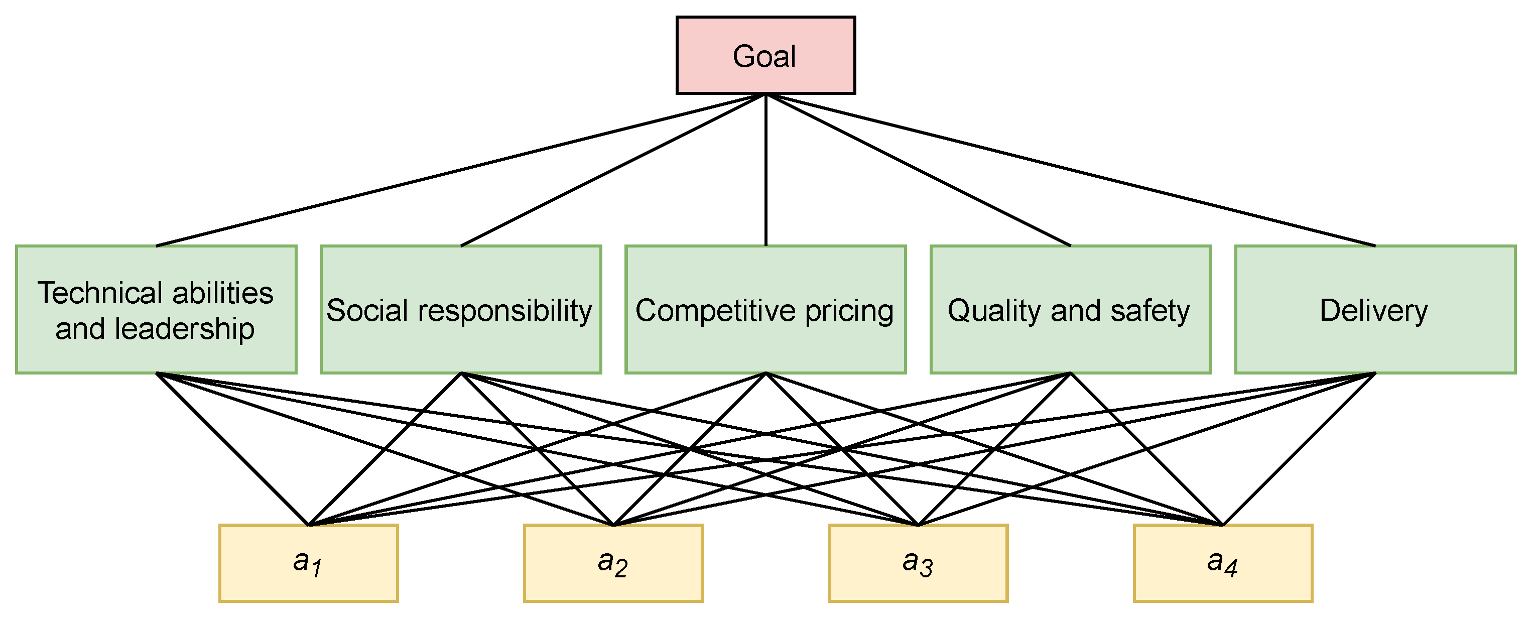
In order to procure important components for new brands, a high-tech manufacturing corporation chooses an appropriate material supplier. After the initial selection, four candidates ($a_1,a_2,a_3,a_4$) proceed to some final analysis. In order to find the most appropriate supplier, a group including experts ($E_1,E_2,E_3$) is established, with the priority weights $\lambda ={(1/3,1/3,1/3)}^T$. Five benefit criteria are considered: (1) technical abilities and leadership ($c_1$); (2) social responsibility ($c_2$); (3) competitive pricing ($c_3$); (4) quality and safety ($c_4$); (5) delivery ($c_5$). The pre-established threshold level $\eta$ of consensus to the set of criteria is $0.75$.

The hierarchical structure for this decision problem can be seen in Figure 1 below.

After the pairwise comparison of the five criteria, the experts provide the following IFPRs:

$R^{\left(1\right)}=\left[\begin{array}{ccccc}0.5& 0.6& r_{13}^1& 0.4& 0.7\\ 0.4& 0.5& r_{23}^1& 0.6& 0.7\\ r_{31}^1& r_{32}^1& 0.5& 0.3& 0.4\\ 0.6& 0.4& 0.7& 0.5& r_{45}^1\\ 0.3& 0.3& 0.6& r_{54}^1& 0.5\end{array}\right];R^{\left(2\right)}=\left[\begin{array}{ccccc}0.5& 0.4& r_{13}^2& 0.6& r_{15}^2\\ 0.6& 0.5& 0.6& 0.5& r_{25}^2\\ r_{31}^2& 0.4& 0.5& 0.3& 0.7\\ 0.4& 0.5& 0.7& 0.5& 0.2\\ r_{51}^2& r_{52}^2& 0.3& 0.8& 0.5\end{array}\right];R^{\left(3\right)}=\left[\begin{array}{ccccc}0.5& 0.3& 0.4& 0.7& 0.7\\ 0.7& 0.5& r_{23}^3& r_{24}^3& r_{25}^3\\ 0.6& r_{32}^3& 0.5& 0.2& 0.8\\ 0.3& r_{42}^3& 0.8& 0.5& 0.3\\ 0.3& r_{52}^3& 0.2& 0.7& 0.5\end{array}\right].$

After the pairwise comparison of the four alternatives for each criterion, the experts provide the following IFPRs:

Technical abilities and leadership:

${}_1{R}^{\left(1\right)}=\left[\begin{array}{cccc}0.5& 0.8& {}_1{r}_{13}^1& {}_1{r}_{14}^1\\ 0.2& 0.5& 0.4& 0.6\\ {}_1{r}_{31}^1& 0.6& 0.5& 0.7\\ {}_1{r}_{41}^1& 0.4& 0.3& 0.5\end{array}\right];{}_1{R}^{\left(2\right)}=\left[\begin{array}{cccc}0.5& 0.7& 1r_{13}^2& 0.6\\ 0.3& 0.5& 0.5& 0.7\\ 1r_{31}^2& 0.5& 0.5& {}_1{r}_{34}^2\\ 0.4& 0.3& {}_1{r}_{43}^2& 0.5\end{array}\right];{}_1{R}^{\left(3\right)}=\left[\begin{array}{cccc}0.5& {}_1{r}_{12}^3& 0.7& {}_1{r}_{14}^3\\ {}_1{r}_{21}^3& 0.5& {}_1{r}_{23}^3& 0.6\\ 0.3& {}_1{r}_{32}^3& 0.5& 0.5\\ {}_1{r}_{41}^3& 0.4& 0.5& 0.5\end{array}\right].$

Social responsibility:

${}_2{R}^{\left(1\right)}=\left[\begin{array}{cccc}0.5& 0.7& 0.5& {}_2{r}_{14}^1\\ 0.3& 0.5& 0.4& 0.6\\ 0.5& 0.6& 0.5& 0.8\\ {}_2{r}_{41}^1& 0.4& 0.2& 0.5\end{array}\right];{}_2{R}^{\left(2\right)}=\left[\begin{array}{cccc}0.5& 0.8& {}_2{r}_{13}^2& {}_2{r}_{14}^2\\ 0.2& 0.5& 0.3& 0.5\\ {}_2{r}_{31}^2& 0.7& 0.5& 0.3\\ {}_2{r}_{41}^2& 0.5& 0.7& 0.5\end{array}\right];{}_2{R}^{\left(3\right)}=\left[\begin{array}{cccc}0.5& 0.9& {}_2{r}_{13}^3& 0.6\\ 0.1& 0.5& 0.4& 0.4\\ {}_2{r}_{31}^3& 0.6& 0.5& {}_2{r}_{34}^3\\ 0.4& 0.6& {}_2{r}_{43}^3& 0.5\end{array}\right].$

Competitive pricing:

${}_3{R}^{\left(1\right)}=\left[\begin{array}{cccc}0.5& 0.6& {}_3{r}_{13}^1& 0.7\\ 0.4& 0.5& 0.3& {}_3{r}_{24}^1\\ {}_3{r}_{31}^1& 0.7& 0.5& 0.4\\ 0.3& {}_3{r}_{42}^1& 0.6& 0.5\end{array}\right];{}_3{R}^{\left(2\right)}=\left[\begin{array}{cccc}0.5& {}_3{r}_{12}^2& {}_3{r}_{13}^2& 0.6\\ {}_3{r}_{21}^2& 0.5& {}_3{r}_{23}^2& 0.2\\ {}_3{r}_{31}^2& {}_3{r}_{32}^2& 0.5& 0.4\\ 0.4& 0.8& 0.6& 0.5\end{array}\right];{}_3{R}^{\left(3\right)}=\left[\begin{array}{cccc}0.5& {}_3{r}_{12}^3& 0.3& 0.5\\ {}_3{r}_{21}^3& 0.5& {}_3{r}_{23}^3& 0.3\\ 0.7& {}_3{r}_{32}^3& 0.5& {}_3{r}_{34}^3\\ 0.5& 0.7& {}_3{r}_{43}^3& 0.5\end{array}\right].$

Quality and safety:

${}_4{R}^{\left(1\right)}=\left[\begin{array}{cccc}0.5& 0.2& {}_4{r}_{13}^1& 0.7\\ 0.8& 0.5& {}_4{r}_{23}^1& {}_4{r}_{24}^1\\ {}_4{r}_{31}^1& {}_4{r}_{32}^1& 0.5& {}_4{r}_{34}^1\\ 0.3& {}_4{r}_{42}^1& {}_4{r}_{43}^1& 0.5\end{array}\right];{}_4{R}^{\left(2\right)}=\left[\begin{array}{cccc}0.5& 0.4& 0.7& {}_4{r}_{14}^2\\ 0.6& 0.5& 0.7& {}_4{r}_{24}^2\\ 0.3& 0.3& 0.5& 0.6\\ {}_4{r}_{41}^2& {}_4{r}_{42}^2& 0.4& 0.5\end{array}\right];{}_4{R}^{\left(3\right)}=\left[\begin{array}{cccc}0.5& {}_4{r}_{12}^3& 0.3& 0.4\\ {}_4{r}_{21}^3& 0.5& 0.2& 0.6\\ 0.7& 0.8& 0.5& {}_4{r}_{34}^3\\ 0.6& 0.4& {}_4{r}_{43}^3& 0.5\end{array}\right].$

Delivery:

${}_5{R}^{\left(1\right)}=\left[\begin{array}{cccc}0.5& {}_5{r}_{12}^1& {}_5{r}_{13}^1& 0.1\\ {}_5{r}_{21}^1& 0.5& 0.4& {}_5{r}_{24}^1\\ {}_5{r}_{31}^1& 0.6& 0.5& 0.7\\ 0.9& {}_5{r}_{42}^1& 0.3& 0.5\end{array}\right];{}_5{R}^{\left(2\right)}=\left[\begin{array}{cccc}0.5& 0.2& {}_5{r}_{13}^2& 0.4\\ 0.8& 0.5& {}_5{r}_{23}^2& 0.3\\ {}_5{r}_{31}^2& {}_5{r}_{32}^2& 0.5& 0.3\\ {}_5{r}_{41}^2& 0.7& 0.7& 0.5\end{array}\right];{}_5{R}^{\left(3\right)}=\left[\begin{array}{cccc}0.5& 0.3& 0.4& {}_5{r}_{14}^3\\ 0.7& 0.5& 0.6& {}_5{r}_{24}^3\\ 0.6& 0.4& 0.5& {}_5{r}_{34}^3\\ {}_5{r}_{41}^3& {}_5{r}_{42}^3& {}_5{r}_{43}^3& 0.5\end{array}\right].$

The use of the suggested method results in the cumulative FPR for five criteria and the corresponding priority weights, as seen in

Table 1. Accumulated fuzzy preference relation (FPR) of criteria and ranking values.

	${\mathit{c}}_1$	${\mathit{c}}_2$	${\mathit{c}}_3$	${\mathit{c}}_4$	${\mathit{c}}_5$	Priority Weights
${\mathbf{c}}_{\mathbf{1}}$	0.50000	0.4358	0.3648	0.5642	0.4658	0.1830
${\mathbf{c}}_{\mathbf{2}}$	0.5642	0.5000	0.3679	0.5017	0.4689	0.1903
${\mathbf{c}}_{\mathbf{3}}$	0.6352	0.6321	0.5000	0.4317	0.6300	0.2329
${\mathbf{c}}_{\mathbf{4}}$	0.4358	0.4983	0.5683	0.5000	0.2666	0.1769
${\mathbf{c}}_{\mathbf{5}}$	0.5342	0.5311	0.3700	0.7334	0.5000	0.2169

, whereas the level of consistency and the degree of consensus for the experts are as follows:

$$T_{L}CI\left(R^1\right)=1;T_{L}CI\left(R^2\right)=0.98;T_{L}CI\left(R^3\right)=0.95,\mathrm{and}CoD=0.7933.$$

The aggregated FPRs for the four suppliers corresponding to the criteria and the priority scores can be seen in

Table 2. Accumulated FPRs for suppliers in relation to each criterion and ranking values.

	${\mathit{a}}_1$	${\mathit{a}}_2$	${\mathit{a}}_3$	${\mathit{a}}_4$	Priority Ratings
$c_1$
$a_1$	0.5000	0.6667	0.3667	0.4000	0.2389
$a_2$	0.3333	0.5000	0.3667	0.6333	0.2222
$a_3$	0.6333	0.6333	0.5000	0.4333	0.2833
$a_4$	0.6000	0.3667	0.5667	0.5000	0.2556
$c_2$
$a_1$	0.5000	0.8000	0.3000	0.4000	0.2500
$a_2$	0.2000	0.5000	0.3667	0.5000	0.1778
$a_3$	0.7000	0.6333	0.5000	0.4667	0.3000
$a_4$	0.6000	0.5000	0.5333	0.5000	0.2722
$c_3$
$a_1$	0.5000	0.4000	0.2667	0.6000	0.2111
$a_2$	0.6000	0.5000	0.1333	0.2000	0.1556
$a_3$	0.7333	0.8667	0.5000	0.3333	0.3222
$a_4$	0.4000	0.8000	0.6667	0.5000	0.3111
$c_4$
$a_1$	0.5000	0.2333	0.5000	0.4667	0.2000
$a_2$	0.7667	0.5000	0.4000	0.4667	0.2722
$a_3$	0.5000	0.6000	0.5000	0.4000	0.2500
$a_4$	0.5333	0.5333	0.6000	0.5000	0.2778
$c_5$
$a_1$	0.5000	0.3333	0.1667	0.3333	0.1389
$a_2$	0.6667	0.5000	0.5000	0.1667	0.2222
$a_3$	0.8333	0.5000	0.5000	0.3667	0.2833
$a_4$	0.6667	0.8333	0.6333	0.5000	0.3556

, and the consistency as well as consensus levels for each criterion are calculated as follows:

Technical abilities and leadership:

$$T_{L}CI{(}_1{R}^1)=1;T_{L}CI{(}_1{R}^2)=1;T_{L}CI{(}_1{R}^3)=1,\mathrm{and}CoD=0.8189.$$

Social responsibility:

$$T_{L}CI{(}_2{R}^1)=1;T_{L}CI{(}_2{R}^2)=1;T_{L}CI{(}_2{R}^3)=1,\mathrm{and}CoD=0.8111.$$

Competitive pricing:

$$T_{L}CI{(}_3{R}^1)=1;T_{L}CI{(}_3{R}^2)=1;T_{L}CI{(}_3{R}^3)=1,\mathrm{and}CoD=0.8445.$$

Quality and safety:

$$T_{L}CI{(}_4{R}^1)=1;T_{L}CI{(}_4{R}^2)=1;T_{L}CI{(}_4{R}^3)=1,\mathrm{and}CoD=0.7933.$$

Delivery:

$$T_{L}CI{(}_5{R}^1)=1;T_{L}CI{(}_5{R}^2)=1;T_{L}CI{(}_5{R}^3)=1,\mathrm{and}CoD=0.7877.$$

The last column of

Table 3. Final priority weights of the four suppliers.

	${\mathit{c}}_1$	${\mathit{c}}_2$	${\mathit{c}}_3$	${\mathit{c}}_4$	${\mathit{c}}_5$	Priority Weights
Criteria weights	0.1830	0.1903	0.2329	0.1769	0.2169
$a_1$	0.2389	0.2500	0.2111	0.2000	0.1389	0.2060
$a_2$	0.2222	0.1778	0.1556	0.2722	0.2222	0.2071
$a_3$	0.2833	0.3000	0.3222	0.2500	0.2833	0.2896
$a_4$	0.2556	0.2722	0.3111	0.2778	0.3556	0.2973

is used to show the final ranking values of the four suppliers, which are $w_{a_1}=0.2060,$$w_{a_2}=0.2071,w_{a_3}=0.2896$ and $w_{a_4}=0.2973$. As $w_{a_4}>w_{a_3}>w_{a_2}>w_{a_1}$; therefore, the ranking order of the four suppliers $a_1,a_2,a_3$ and $a_4$ is $a_4>a_3>a_2>a_1.$

5. Comparison

To validate the productivity of the proposed scheme, we compare the results after concluding the problem taken from [22] with our proposed technique.

Problem Statement

A funds, and five potential candidates (loan users) are in competition for the remaining funds. The problem is to rank the applicants and allocate the loan following the principle of loan allocation until the funds are completely used. A team of five decision makers (DMs) participate in the ranking: the President of the Fund Council (DM1), a senior advisor to the Fund (DM2), the fund manager (DM3), an external expert advisor (DM4) and an expert representative of the Ministry. Three criteria are considered by the team: (1) Service, (2) Loan History (LOANH) and (3) Insurance. After pairwise comparison, the MPRs provided by the DMs are given as presented in

Table 4. Comparison matrices provided by President of the Fund Council (DM1) [22].

Criteria				Service				LOANH				Insurance
Service								2				9
LOANH												5
Insurance
	Service					LOANH					Insurance
	$U_1$	$U_2$	$U_3$	$U_4$	$U_5$	$U_1$	$U_2$	$U_3$	$U_4$	$U_5$	$U_1$	$U_2$	$U_3$	$U_4$	$U_5$
$U_1$		3	1/2	8	4		1/9	1/9	1/4	1/6		2	5	1/2	1/6
$U_2$			1/3	7	3			1	3	2			5	1/3	1/8
$U_3$				9	6				3	2				1/7	1/9
$U_4$					1/4					1/2					1/3
$U_5$

,

Table 5. Comparison matrices provided by Senior advisor of the Fund (DM2) [22].

Criteria				Service				LOANH				Insurance
Service								5				9
LOANH												6
Insurance
	Service					LOANH					Insurance
	$U_1$	$U_2$	$U_3$	$U_4$	$U_5$	$U_1$	$U_2$	$U_3$	$U_4$	$U_5$	$U_1$	$U_2$	$U_3$	$U_4$	$U_5$
$U_1$		4	1/3	6	5		1/6	1/6	1/3	1/3		2	4	1/2	1/4
$U_2$			1/4	5	3			1	2	2			4	1/4	1/6
$U_3$				9	8				2	2				1/8	1/9
$U_4$					1/3					1/2					1/2
$U_5$

,

Table 6. Comparison matrices provided by Fund manager (DM3) [22].

Criteria				Service				LOANH				Insurance
Service								1/5				1/3
LOANH												6
Insurance
	Service					LOANH					Insurance
	$U_1$	$U_2$	$U_3$	$U_4$	$U_5$	$U_1$	$U_2$	$U_3$	$U_4$	$U_5$	$U_1$	$U_2$	$U_3$	$U_4$	$U_5$
$U_1$		2	1/3	7	6		1/5	1/5	1/2	1/4		3	6	1/2	1/7
$U_2$			1/5	5	3			1	2	2			2	1/4	1/7
$U_3$				9	7				2	2				1/6	1/9
$U_4$					1/4					1/2					1/5
$U_5$

,

Table 7. Comparison matrices provided by External expert advisor (DM4) [22].

Criteria				Service				LOANH				Insurance
Service								3				7
LOANH												5
Insurance
	Service					LOANH					Insurance
	$U_1$	$U_2$	$U_3$	$U_4$	$U_5$	$U_1$	$U_2$	$U_3$	$U_4$	$U_5$	$U_1$	$U_2$	$U_3$	$U_4$	$U_5$
$U_1$		3	1/3	8	5		1/8	1/8	1/5	1/6		4	6	1/3	1/5
$U_2$			1/4	6	3			1	3	2			2	1/4	1/7
$U_3$				9	5				3	2				1/6	1/9
$U_4$					1/4					1/3					1/4
$U_5$

and

Table 8. Comparison matrices provided by Expert representative of the Ministry (DM5) [22].

Criteria				Service				LOANH				Insurance
Service								7				9
LOANH												5
Insurance
	Service					LOANH					Insurance
	$U_1$	$U_2$	$U_3$	$U_4$	$U_5$	$U_1$	$U_2$	$U_3$	$U_4$	$U_5$	$U_1$	$U_2$	$U_3$	$U_4$	$U_5$
$U_1$		3	1/5	7	5		1/9	1/9	1/5	1/7		3	6	1/3	1/5
$U_2$			1/6	6	5			1	7	5			4	1/5	1/7
$U_3$				9	7				7	5				1/7	1/9
$U_4$					1/3					1/4					1/4
$U_5$

.

Srdevic et al. [22] determined the ranking oder of five applicants as $U_3>U_2>U_1>U_5>U_4$. However, the priority weights of applicants obtained by the proposed model after transforming the above problem in a fuzzy environment, with the help of Remark 1, are $U_1$ = 0.17781, $U_2$ = 0.23454, $U_3$ = 0.29778, $U_4$ = 0.10693, $U_5$ = 0.18294, which lead to a ranking order of

$$U_3>U_2>U_5>U_1>U_4$$

The result shows that the ranking positions for applicants $U_2$, $U_3$ and $U_4$ are the same as in [22], while the order of applicants $U_1$ and $U_5$ are interchanged, but applicant $U_3$ is the first preference in both models to get the desired loan. The similarities of these two rankings are very high, where the $r_w$ and $WS$ coefficients of the both rankings are equal 0.9167 [47]. There may be two factors that resulted in a different ranking order in few places: (i) different techniques were used to determine the ranking order, and (ii) the corresponding parameters regarding different models could have been evaluated in various ways, and the results may be affected. We think that the proposed model can equally handle complete and incomplete information and provides better results.

6. Conclusions

This paper provides a clear and effective methodology for selecting and ranking suppliers based on a consensus-derived and consistent model for MCGDM in an incomplete AHP environment. The $T_L$-transitivity property plays a main role in evaluating unknown preference values, as it symbolizes one of the most suitable means to model consistent FPRs. $T_{L}CI$ was defined to determine the consistency level of the information provided by each expert. The proposed method was used in three steps: firstly, we evaluated the priority weight vector of criteria; secondly, we estimated the priority ratings of each alternative against each criterion; finally, we determined the priority weight vector for alternatives, which allowed us to obtain the best alternative. At the end of this study, we successfully applied the proposed procedure to select a suitable supplier in SCM by illustrating a numerical example to highlight the practicability and efficacy of the method.

In summary, the proposed method has the following major advantages: (i) in this manuscript, $T_L$-transitivity was considered to measure the FPRs’ unspecified preference values. $T_L$-transitivity is more suitable to model consistent FPRs compared with other consistency-based techniques; (ii) the consistency degrees of experts’ opinions were measured to strengthen the final decision; (iii) after reaching the required level of consensus among the experts, first, a ranking of the criteria was established, and then alternatives were prioritized under each criterion based on the consistent information.

To the best of our knowledge, a similar method to deal with MCGDM problems using the AHP model has not previously been proposed. From our perspective, this procedure is an efficient and reliable way to gain a greater insight to solve MCGDM problems in the current environment. This study suffers from limitations that should be addressed in future work: (i) experts might exhibit a degree of hesitancy while providing their preferences—it will be interesting to develop procedures to deal with MCGDM in AHP under hesitant fuzzy preference relations; (ii) the threshold consensus degree $\eta$ has a direct influence on the consensus round but is typically evaluated in advance—it will be interesting to observe how this parameter can be estimated based on different factors; (iii) there are some risks that some experts may provide their information dishonestly or refuse to make changes with the preferences. Thus, some mechanism may be introduced to handle non-cooperative activities in consensus-building. We will try to work in the above-mentioned directions to face future challenges; these will contribute to the acceptance of this research area.

References

- Durmić, E.; Stević, Ž.; Chatterjee, P.; Vasiljević, M.; Tomašević, M. Sustainable supplier selection using combined FUCOM—Rough SAW model. Rep. Mech. Eng. 2020, 1, 34–43. [Google Scholar] [CrossRef]
- Sałabun, W.; Ziemba, P. Application of the Characteristic Objects Method in Supply Chain Management and Logistics. In Recent Developments in Intelligent Information and Database Systems; Springer: Berlin/Heidelberg, Germany, 2016; pp. 445–453. [Google Scholar]
- Badi, I.; Pamucar, D. Supplier selection for steelmaking company by using combined Grey-MARCOS methods. Decis. Mak. Appl. Manag. Eng. 2020, 3, 37–48. [Google Scholar] [CrossRef]
- Chakraborty, S.; Chattopadhyay, R.; Chakraborty, S. An integrated D-MARCOS method for supplier selection in an iron and steel industry. Decis. Mak. Appl. Manag. Eng. 2020, 3, 49–69. [Google Scholar]
- Swaminathan, J.M.; Tayur, S.R. Models for supply chains in e-business. Manage. Sci. 2003, 49, 1387–1406. [Google Scholar] [CrossRef] [Green Version]
- Chen, C.T.; Lin, C.T.; Huang, S.F. A fuzzy approach for supplier evaluation & selection in supply chain management. Int. J. Prod. Econ. 2006, 102, 289–301. [Google Scholar]
- De Boer, L.; Labro, E.; Morlacchi, P. A review of methods supporting supplier selection. Eur. J. Purch. Supply Manag. 2001, 7, 75–89. [Google Scholar] [CrossRef]
- Demirtas, E.; Üstün, Ö. An integrated multiobjective decision making process for supplier selection and order allocation. Omega 2008, 36, 76–90. [Google Scholar] [CrossRef]
- Hwang, C.L.; Yoon, K. Multiple Attributes Decision Making Methods & Applications; Springer: New York, NY, USA, 1981. [Google Scholar]
- Ng, W.L. An efficient & simple model for multiple criteria supplier selection problem. Eur. J. Oper. Res. 2008, 186, 1059–1067. [Google Scholar]
- Dickson, G.W. A analysis of vender selection systems & decisions. J. Suppl. Chain Manag. 1966, 2, 5–17. [Google Scholar]
- Barbarosoglu, G.; Yazgaç, T. An application of the analytic hierarchy process to the supplier selection problem. Prod. Inventory Manag. J. 1997, 38, 14–21. [Google Scholar]
- Goffin, K.; Szwejczewski, M.; New, C. Managing suppliers when fewer can mean more. Int. J. Phys. Distrib. Logist. Manag. 1997, 27, 422–436. [Google Scholar] [CrossRef]
- Swift, C.O. Preference for single sourcing & supplier selection criteria. J. Bus. Res. 1995, 32, 105–111. [Google Scholar]
- Weber, C.A.; Current, J.R.; Benton, W.C. Vender selection criteria & method. Eur. J. Oper. Res. 1991, 50, 2–18. [Google Scholar]
- Chai, J.; Liu, J.N.K.; Ngai, E.W.T. Application of decision-making techniques in supplier selection: A systematic review of literature. Expert Syst. Appl. 2013, 40, 3872–3885. [Google Scholar] [CrossRef]
- Faizi, S.; Sałabun, W.; Rashid, T.; Wątróbski, J.; Zafar, S. Group decision-making for hesitant fuzzy sets based on characteristic objects method. Symmetry 2017, 9, 136. [Google Scholar] [CrossRef]
- Faizi, S.; Sałabun, W.; Rashid, T.; Zafar, S.; Wątróbski, J. Intuitionistic fuzzy sets in multi-criteria group decision making problems using the characteristic objects method. Symmetry 2020, 12, 1382. [Google Scholar] [CrossRef]
- Chen, P.C. A fuzzy multiple criteria decision making model in employee recruitment. Int. J. Comput. Sci. Net. Secur. 2009, 9, 113–117. [Google Scholar]
- Hadi-Vencheh, A.; Mokhtarian, M.N. A new fuzzy MCDM approach based on centroid of fuzzy numbers. Expert Syst. Appl. 2011, 38, 5226–5230. [Google Scholar] [CrossRef]
- Önüt, S.; Efendigil, T.; Kara, S.S. A combined fuzzy MCDM approach for selecting shopping center site: An example from Istanbul, Turkey. Expert Syst. Appl. 2010, 37, 1973–1980. [Google Scholar] [CrossRef]
- Srdevic, Z.; Blagojevic, B.; Srdevic, B. AHP based group decision making in ranking loan applicants for purchasing irrigation equipment: A case study. Bulg. J. Agric. Sci. 2011, 17, 531–543. [Google Scholar]
- Sun, C.C.; Lin, G.T.R.; Tzeng, G.H. The evaluation of cluster policy by fuzzy MCDM: Empirical evidence from Hsin Chu Science Park. Expert Syst. Appl. 2009, 36, 11895–11906. [Google Scholar] [CrossRef]
- Wu, H.Y.; Tzeng, G.H.; Chen, Y.H. A fuzzy MCDM approach for evaluating banking performance based on balanced scorecard. Expert Syst. Appl. 2009, 36, 10135–10147. [Google Scholar] [CrossRef]
- Bashir, Z.; Rashid, T.; Wątróbski, J. Sałabun, W.; Malik, A. Hesitant probabilistic multiplicative preference relations in group decision making. Appl. Sci. 2018, 8, 398. [Google Scholar] [CrossRef] [Green Version]
- Kim, S.H.; Ahn, B.S. Interactive group decision making procedure under incomplete information. Eur. J. Oper. Res. 1999, 116, 498–507. [Google Scholar] [CrossRef]
- Xu, Z.S. Goal programming models for obtaining the priority vector of incomplete fuzzy preference relation. Int. J. Approx. Reason. 2004, 36, 261–270. [Google Scholar] [CrossRef] [Green Version]
- Gong, Z.W. Least-square method to priority of the fuzzy preference relations with incomplete information. Int. J. Approx. Reason. 2008, 47, 258–264. [Google Scholar] [CrossRef] [Green Version]
- Herrera-Viedma, E.; Chiclana, F.; Herrera, F.; Alonso, S. Group decision-making model with incomplete fuzzy preference relations based on additive consistency. IEEE Trans. Syst. Man Cybern. Part B Cybern. 2007, 37, 176–189. [Google Scholar] [CrossRef]
- Alonso, S.; Chiclana, F.; Herrera, F.; Herrera-Viedma, E. A consistency based procedure to estimate missing pairwise preference values. Int. J. Intell. Syst. 2008, 23, 155–175. [Google Scholar] [CrossRef]
- Xu, Y.J. On group decision making with four formats of incomplete preference relations. Comput. Ind. Eng. 2011, 61, 48–54. [Google Scholar] [CrossRef]
- Lee, L.W. Group decision making with incomplete fuzzy preference relations based on the additive consistency and the order consistency. Expert Syst. Appl. 2012, 39, 11666–11676. [Google Scholar] [CrossRef]
- Chen, S.M.; Lin, T.E.; Lee, L.W. Group decision making using incomplete fuzzy preference relations based on the additive consistency and the order consistency. Inf. Sci. 2014, 259, 1–15. [Google Scholar] [CrossRef]
- Rehman, A.; Kerre, E.E.; Ashraf, S. Group decision making by using incomplete fuzzy preference relations based on T-Consistency Order Consistency. Int. J. Intell. Syst. 2015, 30, 120–143. [Google Scholar] [CrossRef] [Green Version]
- Kerre, E.E.; Rehman, A.U.; Ashraf, S. Group decision making with incomplete reciprocal preference relations based on multiplicative consistency. Int. J. Comput. Intell. Syst. 2018, 11, 1030–1040. [Google Scholar] [CrossRef] [Green Version]
- Saaty, T.L. The Analytic Hierarchy Process: Planning, Priority Setting & Resource Allocation; ; McGraw-Hill: New York, NY, USA, 1980. [Google Scholar]
- Saaty, T.L. How to make a decision: The analytic hierarchy process. Eur. J. Oper. Res. 1990, 48, 9–26. [Google Scholar] [CrossRef]
- Lin, C.T.; Hsu, P.F. Adopting an analytic hierarchy process to select internet advertising networks. Mark. Intell. Plan. 2003, 21, 183–191. [Google Scholar] [CrossRef]
- Omasa, T.; Kisshimoto, M.; Kawase, M.; Yagi, K. An attempt at decision making in tissue engineering: Reactor evaluation using the analytic hierarchy process (AHP). Biochem. Eng. J. 2004, 20, 173–179. [Google Scholar] [CrossRef]
- Wei, C.C.; Chien, C.F.; Wang, M.J. An AHP-based approach to ERP system selection. Int. J. Prod. Econ. 2005, 96, 47–62. [Google Scholar] [CrossRef]
- Tanino, T. Fuzzy preference relations in group decision making. In Non-Conventional Preference Relations in Decision Making; Lecture Notes in Economics and Mathematical Systems; Springer: Berlin/Heidelberg, Germany, 1988; Volume 301, pp. 54–71. [Google Scholar]
- Venugopalan, P. Fuzzy ordered sets. Fuzzy Sets Syst. 1992, 46, 221–226. [Google Scholar] [CrossRef]
- Zadeh, L.A. Fuzzy sets. Inf. Control 1965, 8, 338–353. [Google Scholar] [CrossRef] [Green Version]
- Tanino, T. Fuzzy preference orderings in group decision making. Fuzzy Sets Syst. 1984, 12, 117–131. [Google Scholar] [CrossRef]
- Ureña, R.; Chiclana, F.; Alonso, S.; Morente-Molinera, J.A.; Herrera-Viedma, E. On incomplete fuzzy and multiplicative preference relations in multi-person decision making. Procedia Comput. Sci. 2014, 31, 793–801. [Google Scholar] [CrossRef] [Green Version]
- Zhang, X.; Ge, B.; Jiang, J.; Tan, Y. Consensus building in group decision making based on multiplicative consistency with incomplete reciprocal preference relations. Knowl.-Based Syst. 2016, 106, 96–104. [Google Scholar] [CrossRef]
- Sałabun, W.; Urbaniak, K. A new coefficient of rankings similarity in decision-making problems. In International Conference on Computational Science; Springer: Cham, Switzerland, 2020; pp. 632–645. [Google Scholar]