Blade Sorting Method for Unbalance Minimization of an Aeroengine Concentric Rotor

Abstract

This paper proposes a blade sorting method based on the cloud adaptive genetic algorithm (CAGA), which is used to optimize the unbalanced of asymmetric rotor of aero-engine. Firstly, by analyzing the unbalance of the arrangement caused by the deviation of the mass moment of the blade, and considering the concentricity of the disk, an optimization model of the unbalanced amount of the blade assembly was established. Secondly, the selection operator, crossover operator, and mutation operator of the algorithm were designed, and the cloud adaptive genetic algorithm was used to optimize the assembly unbalance. Thirdly, the mass moments of a group of aero-engine blades were weighed using a moment scale (MW0), and the blade mass moment distribution and assembly unbalance under the six blade arrangements were analyzed. Finally, by setting different disk concentricity, the corresponding blade arrangement and the final rotor unbalance were obtained. Through analysis, it was found that the unbalance of GA is at least 57.5% optimized relative to the weight sorted, sorting type 2, sorting type 4, and sorting-1/4 skip method, and the unbalance optimized by the CAGA is 95.7% optimized relative to GA. In the case of different initial concentricity of the disk, the effective algorithm accuracy is still maintained, which proves the effectiveness of the method for the arrangement of asymmetric rotor blades. This method establishes an effective asymmetric rotor blade arrangement model, uses the cloud adaptive genetic algorithm to sort the blade assembly, and effectively reduces the unbalanced amount of the asymmetric rotor.

1. Introduction

The optimization of aero-engine rotor unbalance is an important part of the assembly process [1,2,3]. Blades need to work under a high-load, high-speed, and high-vibration environment, which directly affects the start-stop performance, working reliability, efficiency, and cost of the aero-engine. The blades have the characteristics of complex shapes and high precision requirements. Therefore, in the production process, in order to meet the technological requirements, the blades need to be manually polished, so that the mass moment of each blade after assembly is different, resulting in the overall rotor having a large residual unbalance. Therefore, a reasonable blade arrangement can reduce the unbalance of the rotor, and a large number of scholars have done research in this area [4]. Piskin et al. introduced the grouping methods of blade assembly. These methods optimize the imbalance of the rotor and provide a basis for the application of intelligent algorithms [5,6]. Lavagnoli developed a numerical strategy to select the best blade arrangement around the rotor, taking into account the measured blade weight distribution and any residual disk unbalance, which makes the algorithm calculate the best blade sort in the fan-constrained rotor row in a few seconds [7]. Amiouny developed a heuristic of a problem that models the static balance of a turbofan: load point mass at regularly spaced locations on the circumference so that the residual imbalance around the center corresponding to the fan’s axis of rotation is as small as possible [8]. Pitsoulis proposed a heuristic algorithm to solve an NP-Hard combinatorial optimization problem in turbine engine manufacturing and maintenance [9].

Li et al. used the ant colony algorithm to find the blade arrangement, and successfully reduced the impeller unbalance over one year to 1% of the standard value, and the impeller unbalance over 99% was reduced to 1% of the official value [10,11]. Mason used a neighborhood search algorithm to determine the best position of the turbine blades, so that the total time required for balancing could be significantly reduced. It also showed that using the starting points obtained from the Lagrangian dual scheme can greatly improve the results of the problem [12]. Thompson et al. used the simulated annealing algorithm to solve the large-scale combinatorial optimization problem of seeking the best layout through blade exchange [13,14,15]. Dai et al. applied it to the optimal arrangement of blades of impeller machinery on the basis of the genetic algorithm, which solved the problem of a long solution time and an inability to obtain optimization results that were encountered in the previous optimization of a large number of blades by the exhaustive method [16,17,18]. Pan et al. improved the genetic algorithm based on the genetic algorithm, and proposed an improved genetic algorithm to solve the assembly sort optimization problem [19,20,21]. Wang improved the non-dominated sorting genetic algorithm (NSGA), introduced the control elite and dynamic crowding distance, and showed good performance when dealing with multi-objective optimization problems of wind turbines [22]. In this paper, we use a cloud adaptive genetic algorithm (CAGA) to solve the blade sorting problem for the rotor unbalance situation, and its convergence speed and sorting results are explained.

The structure of this paper is as follows. Firstly, the vector sum model of blade mass moment and eccentric moment is established to obtain the unbalanced optimization function. Secondly, the cloud adaptive genetic algorithm is used to optimize the rotor unbalance, and the blade sort corresponding to the minimum unbalance is given. Finally, combined with the blade mass moment weighed by the torque, the effectiveness of the method is verified by comparing six commonly used blade arrangement methods.

2. Blade Assembly Mass Moment Model

2.1. Physical Model of Blade Sorting Based on Mass Moment

Blade balancing is an important task in aero-engine rotor assembly. The blades are machined and then are assembled on the blade disk to form a rotor. The residual unbalance of the bladed rotor should be balanced to be as small as possible. In the blade production process, mass moment unbalance is generated. The geometry size, shape contour, mass distribution, centroid deviation, and installation position of each blade are different so that the non-zero centrifugal force vectors of the blades result in instability of the aero-engine. Figure 1 shows a random blade sorting model. The mass moments of two blades in the diagonal lines (No. 1–5, 2–6, 3–7, 4–8) are obviously different and the residual unbalance of the bladed rotor is very large.

As shown in Figure 2, an optimum sorting model is given to obtain minimization torque. We sort a pair of blades with similar mass moments in the diagonal lines so that the mass moment vectors of the blade pairs (No. 1–2, 3–4, 5–6, 7–8) can be cancelled symmetrically and the residual unbalance of the bladed rotor is minimal.

Ideally, the centrifugal forces generated by the blades are balanced to zero, that is, the vector sum of centrifugal force is 0, as shown in Equation (1):

$$F={\displaystyle \sum F_i}={\displaystyle \sum m_i\times {\omega }^2\times \overrightarrow{r_i}}=0$$

(1)

where m_i is the mass of each blade, r_i is the radius of the gravity center of each blade, and ω is the rotation angular velocity.

Since the rotation angular velocity ω is the same for the whole aero-engine rotor system, Equation (1) can be simplified to Equation (2):

$$\sum m_i\times \overrightarrow{r_i}=0$$

(2)

We define m_i × r_i as the mass moment vector, that is, the product of the blade mass and the distance from blade gravity center to the rotor axis. It can be seen from Equation (2) and Figure 2 that mass moment vectors of all the blades can be cancelled out and the minimum unbalance obtained.

The torque vector sum of the random sorting (Figure 3) and the torque minimization model sorting (Figure 4) of the installed blades given above is as follows. By comparing and analyzing the final unbalance of Figure 3 and Figure 4, it is shown that reasonable blade classification can reduce the imbalance of the components.

To facilitate the fitness function, the unbalance can be expressed as:

$$M={\displaystyle \sum _{i=1}^n{m}_i\times {\overrightarrow{r}}_i}={\displaystyle \sum _{i=1}^n{m}_i(x_i+j{y}_i)}={\displaystyle \sum _{i=1}^n{m}_i{x}_i}+j{\displaystyle \sum _{i=1}^n{m}_i{y}_i}={\overrightarrow{M}}_x+j{\overrightarrow{M}}_y$$

(3)

$$\{\begin{array}{l}{m}_i{x}_i=m_i{r}_i\cos \theta =m_i{r}_i\cos (\frac{2\pi (i-1)}{n})\\ m_i{y}_i=m_i{r}_i\sin \theta =m_i{r}_i\sin (\frac{2\pi (i-1)}{n})\end{array}$$

(4)

$$\{\begin{array}{c}{\overrightarrow{M}}_x={\displaystyle \sum _{i=1}^n{m}_i{x}_i}\\ {\overrightarrow{M}}_y={\displaystyle \sum _{i=1}^n{m}_i{y}_i}\end{array}$$

(5)

where m_i × r_i is the mass moment of the i-th blade, x_i and y_i are the X-axis and Y-axis coordinates of the centroid of the i-th blade, and m_ix_i and m_iy_i are the components of the mass moment of the i-th blade on the X-axis and Y-axis, respectively.

Our goal is to obtain the minimum mass moment unbalance of all the blades:

$$Z=\min \overrightarrow{M}=\left|{\overrightarrow{M}}_x+j{\overrightarrow{M}}_y\right|=\sqrt{M_x{}^2+M_y{}^2}$$

(6)

2.2. Physical Model of Blade Assembly on Asymmetric Disk

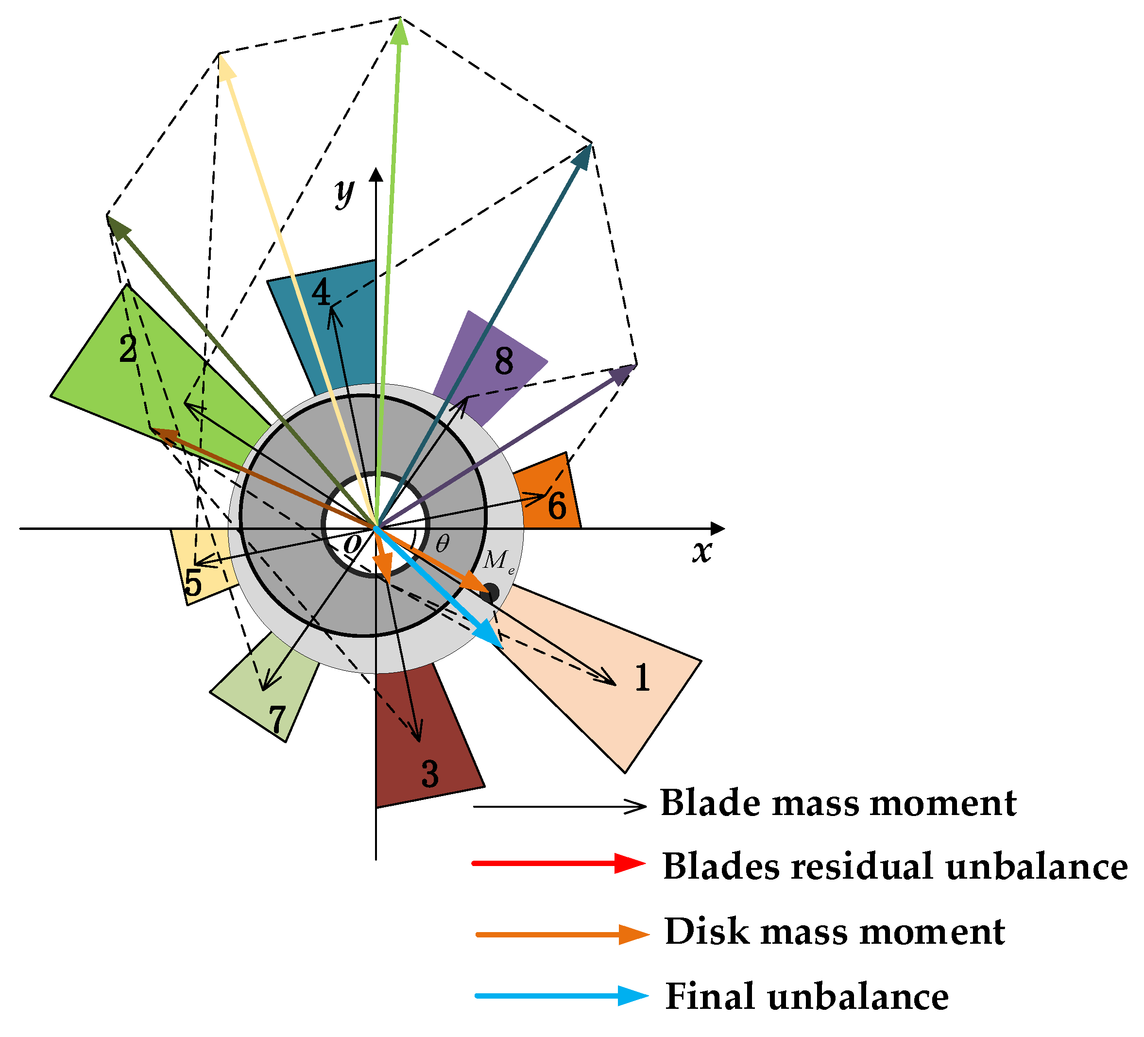
Ideally, the disk is symmetrical. In fact, the disk is asymmetrical due to processing errors. Before the best sorting of the blades, we should consider the unbalance of the mass moment of the blades and the concentricity of the disk at the same time, that is, the asymmetry of the rotor system. Our best classification goal is to obtain the smallest unbalance after the blade is assembled on the disk. The vector sum models of the mass moment of the disk with random and optimum are shown in Figure 5 and Figure 6, respectively.

Comparing Figure 5 and Figure 6, we can see that the disk mass moment destroys the minimum unbalance of optimal blade sorting. How to obtain the minimum unbalance of the whole bladed disk is the subject of the next study.

It can be seen from Figure 5 and Figure 6 that the minimum unbalance under the consideration of the eccentric mass moment of the disk is:

$${\overrightarrow{M}}_1=\overrightarrow{M}+{\overrightarrow{M}}_e$$

(7)

$$Z_1=\min \left|\overrightarrow{M}+{\overrightarrow{M}}_e\right|=\sqrt{{(M_x+M_{ex})}^2+{(M_y+M_{ey})}^2}$$

(8)

$$\{\begin{array}{c}{M}_{ex}=M_e\cos {\theta }_1\\ M_{ey}=M_e\sin {\theta }_1\end{array}$$

(9)

where M_e is the mass moment of the disk, and θ₁ is the angle between M_e and the positive direction of the X-axis.

Regardless of the blade mounting error, the angle between the first blade mounting position and the blade disk mass moment is 30°; then:

$${\theta }_1={\theta }_2-\frac{2\pi }{n}(i-1)$$

(10)

$$M_{ex}=M_e\cos ({\theta }_2-\frac{2\pi }{n}(i-1))$$

(11)

$$M_{ey}=M_e\sin ({\theta }_2-\frac{2\pi }{n}(i-1))$$

(12)

2.3. Optimization Sorting Model

The blade sequencing problem is a kind of linear programming problem in combinatorial optimization. The optimization goal of the problem is how to assign to minimize the total cost of the work. Specifically, it can be described that a blade can only be installed in one position, so there is an unbalance on this position. How to arrange all the blades is to obtain the total minimized unbalance. Resources i(I = 1,2,…,n) can only be uniquely assigned to work k(k = 1,2,…,n) at a certain time, resulting in a corresponding cost c_ik. The relationship between the blade and installation position is expressed by the 0–1 variable x_ik:

$$x_{ik}=\{\begin{array}{c}1\begin{array}{cccc}& & & i=k\end{array}\\ 0\begin{array}{cccc}& & & i\ne k\end{array}\end{array}$$

(13)

The optimizing objective function and constraint function can be expressed as:

$$\begin{gathered} \min {\displaystyle \sum _{i=1}^n{\displaystyle \sum _{k=1}^n{c}_{ik}}}{x}_{ik} \\ sub.to\{\begin{array}{c}{\displaystyle \sum _{i=1}^n{x}_{ik}=1\begin{array}{cccc}& & & i=1,2,\cdots ,n\end{array}}\\ {\displaystyle \sum _{j=1}^n{x}_{jk}=1\begin{array}{cccc}& & & k=1,2,\cdots ,n\end{array}}\\ x_{ik}=0,1\begin{array}{cccc}& & & i,k=1,2,\cdots ,n\end{array}\end{array} \end{gathered}$$

(14)

3. Cloud Adaptive Genetic Algorithm

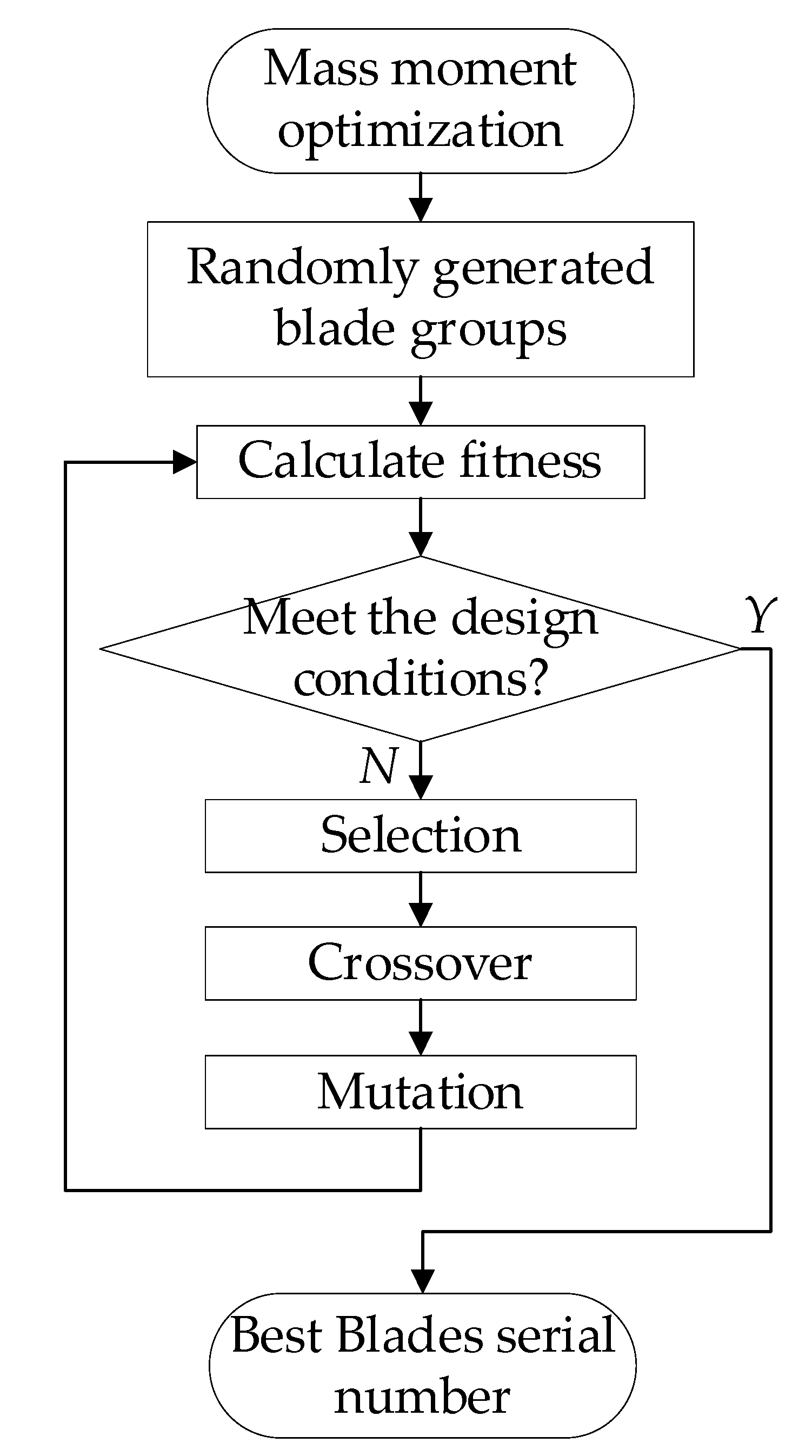
The genetic algorithm (GA) was first proposed by the American professor Holland in 1975 [23]. It is a kind of random search algorithm that draws lessons from natural selection and the natural genetic mechanism in the biological world. The genetic algorithm simulates the selection, crossover, and mutation phenomena of natural selection and the genetic process. Each iteration of blades with a set of candidate solutions, the optimal chromosomes are selected according to the indicators, and these chromosomes are combined with genetic operators to generate a new generation of candidate groups. The process is repeated until the convergence index is satisfied. The specific flow chart is shown in Figure 7.

The initial population is the size of the search area, which determines the search time and search accuracy. Fitness is the only measure of population evolution. The greater the population fitness, the higher the accuracy of the search results. The number of iterations is used as the number of population updates. The selection operation selects individuals with high fitness from the parent population as the offspring. The crossover operation randomly selects the two chromosomes left by the selection operation for gene exchange, thereby forming a new individual and placing it in the offspring. The mutation operation randomly selects the chromosomes in the selection operation for gene mutation, to form a new individual. Both crossover and mutation operations have crossover probability and mutation probability to determine whether to perform the operation.

Genetic algorithm has the characteristics of a low order, short defining moment, and high average fitness. If the probability of crossover and mutation is small and the fitness is low, it is difficult to produce excellent new chromosomes. If a large crossover and mutation probability are adopted, the population will easily fall into local optimization. Therefore, the adaptive genetic algorithm (AGA) appeared, while AGA only considers the trend of the evolutionary process and ignores the randomness of environmental evolution.

The cloud adaptive genetic algorithm improves the above defects. It adopts the cloud model theory [24]. The cloud model is a set of random numbers with stable regularity following the regular distribution law, represented by the expected value (Ex), entropy (En), and hyper entropy (He). The cloud model makes use of the uncertain transformation model between qualitative and quantitative concepts of linguistic values, which is both random and fuzzy, and provides an effective means for the combination of qualitative and quantitative information. It is mainly reflected in the crossover and mutation operators of the genetic algorithm.

3.1. The Coding and Operation of the Genetic Algorithm for Optimal Blade Sorting

In this paper, N sets of blades were randomly generated as the initial population. Each blade is equivalent to a chromosome, which has a certain code. Sequential coding is adopted in blade sorting, that is, there is a one-to-one correspondence between the blade and feasible position. Since the wheel disk is a circle, it is stipulated that the position that coincides with the positive direction of the X-axis is the first position, and the counterclockwise direction is the positive direction of blade installation. The sorting scheme given in Figure 2 is [6, 8, 4, 2, 5, 7, 3, 1].

3.1.1. Selection

The selection reflects the survival principle of the fittest. It retains large fitness and eliminates low fitness chromosomes. Its role is to avoid gene deletion, and improve the global convergence and computational efficiency. In this paper, the operator is selected using roulette, and chromosomes with large fitness are highly likely to be selected. For each chromosome, if its fitness value is f(x_i), then the relative value of its fitness is:

$$p_i=\frac{f(x_i)}{{\displaystyle \sum _{i=1}^{pop}f(x_i)}}$$

(15)

where pop is the size of the population, and we take A as the selection probability of selecting this chromosome. The specific operation of the roulette blade selection is: Accumulate the chromosome’s selection probability(p_i) one by one to get the cumulative probability(p_j), and divide the interval [0–1] into pop intervals. Then, generate a random number belonging to [0–1]. If the number falls in the interval [p_j−1, p_j], select the chromosome corresponding to p_j. For example, if the selection probabilities of chromosomes A, B, C, and D are 0.1, 0.2, 0.3, and 0.4, then their cumulative probabilities set the interval to [0–0.1], [0.1–0.3], [0.3–0.6], and [0.6–1]. If the random number is 0.5, then the chromosome C is selected.

3.1.2. Crossover

Crossover allows the exchange of genetic material between chromosomes to produce better chromosomes. In this paper, a blade is regarded as a gene in a chromosome, so two blades of the same code cannot appear in a chromosome. General single-point crossover operators and multi-point crossover operators are obviously not eligible, so we use the recombination crossover operator. This method first builds an edge list for the blades in the two parent chromosomes, indicating the blades connected to this blade and the number of occurrences. Assume two parental chromosomes are:

P1 = (1,2,3,4,5,6,7,8)

P2 = (3,8,1,6,5,4,7,2)

The two chromosomes are crossed, and the resulting edge list is shown in

Table 1. Blade edge list.

Blade	Adjacent Blades	Blade	Adjacent Blades
1	2, −8, 6	5	−4, −6
2	1, 7, −3	6	1, 7, −5
3	−2, 4, 8	7	4, 6, 2, 8
4	3, −5, 7	8	−1, 3, 7

. If an edge appears twice in the parents, a “−” sign is added to the vertex of the edge in the list. The edge recombination crossover operator starts constructing offspring by selecting an initial point.

We can choose the first position of the parent (P₁) as the starting point of the descendants. Then, the offspring (C₁) is:

C₁ = (1,#,#,#,#,#,#,#)

The principle of selecting a chromosome from the parents is to select the blade with the least number of blades adjacent to it. If the number of blades connected to a certain two are equal, the blade with “−” is preferred. If the above conditions are the same for both blades, then one of them is selected at random. As shown by P₁ and P₂, there are two, six, and eight blades connected to blade 1. They have the same number of blades, but there is a “−” sign before eight, so eight is chosen. There are one, three, and seven blades connected to eight, and one has been selected before, so we chose between three and seven; because there are more adjacent blades to seven, we chose three. Repeatedly, we can get:

C1 = (1,8,3,2,7,6,5,4)

The crossover probability(p_c) is given by the cloud adaptive genetic algorithm:

$$\{\begin{array}{l}{p}_c=\{\begin{array}{c}{k}_{1}e\frac{-{(f^{\prime }-Ex)}^2}{2{(E{n}^{\prime })}^2}\begin{array}{cccc}& & & f^{\prime }\ge \overline{f}\end{array}\\ k_3\begin{array}{cccc}& & \begin{array}{ccc}\begin{array}{ccc}& & \end{array}& & \end{array}& f^{\prime }<\overline{f}\end{array}\end{array}\\ s.t.\{\begin{array}{l}Ex=\overline{f}\\ En=(f_{\max }-\overline{f})/c_1\\ He=En/c_2\\ E{n}^{\prime }=RANDN(En,He)\end{array}\end{array}$$

(16)

3.1.3. Mutation

The mutation can restore the lost or untapped genetic material of the chromosome to prevent the chromosome from converging prematurely during the formation of the optimal solution. For the problem of blade arrangement, this paper uses a two-element optimization mutation operator. That is, the chromosomes selected according to the mutation probability are randomly selected at a certain position of the chromosome to exchange blades, and a new blade order is obtained. All the chromosomes of the parents are mutated according to the mutation probability until the next generation population is generated. The mutation probability(p_m) is given by the cloud adaptive genetic algorithm:

$$\{\begin{array}{l}{p}_m=\{\begin{array}{c}{k}_{2}e\frac{-{(f-Ex)}^2}{2{(E{n}^{\prime })}^2}\begin{array}{cccc}& & & f\ge \overline{f}\end{array}\\ k_4\begin{array}{cccc}& & \begin{array}{ccc}\begin{array}{ccc}& & \end{array}& & \end{array}& f<\overline{f}\end{array}\end{array}\\ s.t.\{\begin{array}{l}Ex=f\\ En=(f_{\max }-\overline{f})/c_3\\ He=En/c_4\\ E{n}^{\prime }=RANDN(En,He)\end{array}\end{array}$$

(17)

where RANDN(En,He) generates a normal random number with an expected value of En and a standard deviation of He. f_max is the maximum fitness of the population, $\overline{f}$ is the average fitness, f′ is the fitness of the mutant chromosomes, and f is the larger value of the fitness of the crossed chromosomes, k₁~k₄ ε[0~1]. In this paper, k₁ = k₃ = 1.0, k₂ = k₄ = 0.5, c₁ = 2.9, c₃ = 3.0, c₂ = c₄ = 10.

3.2. Fitness Function

According to the principle of biological evolution, the larger the fitness requirement, the better, and it is non-negative. Combined with the total unbalance given above, the fitness function given in this paper is as follows:

$$f=\frac{1}{Z_1}=\frac{1}{\left|M_{1x}+i{M}_{1y}\right|}=\frac{1}{\sqrt{{(M_x+M_{ex})}^2+{(M_y+M_{ey})}^2}}$$

(18)

4. Data Validation

In order to view the actual optimization effect and calculation speed of the algorithm, the blades of the first-stage rotor of an aeroengine were selected for cloud adaptive genetic algorithm assembly optimization. Due to special requirements, we cannot disclose the test pieces of blades and disk, so we used the rotor in Figure 8 as the experimental schematic diagram. There are 32 blades in this group. The mass moment of this group of blades was measured on the mass moment scale (MW0). The value is shown in

Table 2. Mass moment values of aeroengine blades.

Serial Number	Mass Moment (g.mm)	Serial Number	Mass Moment (g.mm)	Serial Number	Mass Moment (g.mm)	Serial Number	Mass Moment (g.mm)
1	1,762,040	9	1,762,720	17	1,757,760	25	1,749,600
2	1,761,980	10	1,758,240	18	1,762,280	26	1,779,360
3	1,726,720	11	1,758,040	19	1,769,660	27	1,756,400
4	1,755,640	12	1,740,860	20	1,754,920	28	1,767,280
5	1,755,000	13	1,754,680	21	1,757,900	29	1,756,540
6	1,756,880	14	1,742,080	22	1,761,320	30	1,758,020
7	1,762,720	15	1,754,580	23	1,755,700	31	1,772,240
8	1,762,200	16	1,754,380	24	1,754,700	32	1,772,960

.

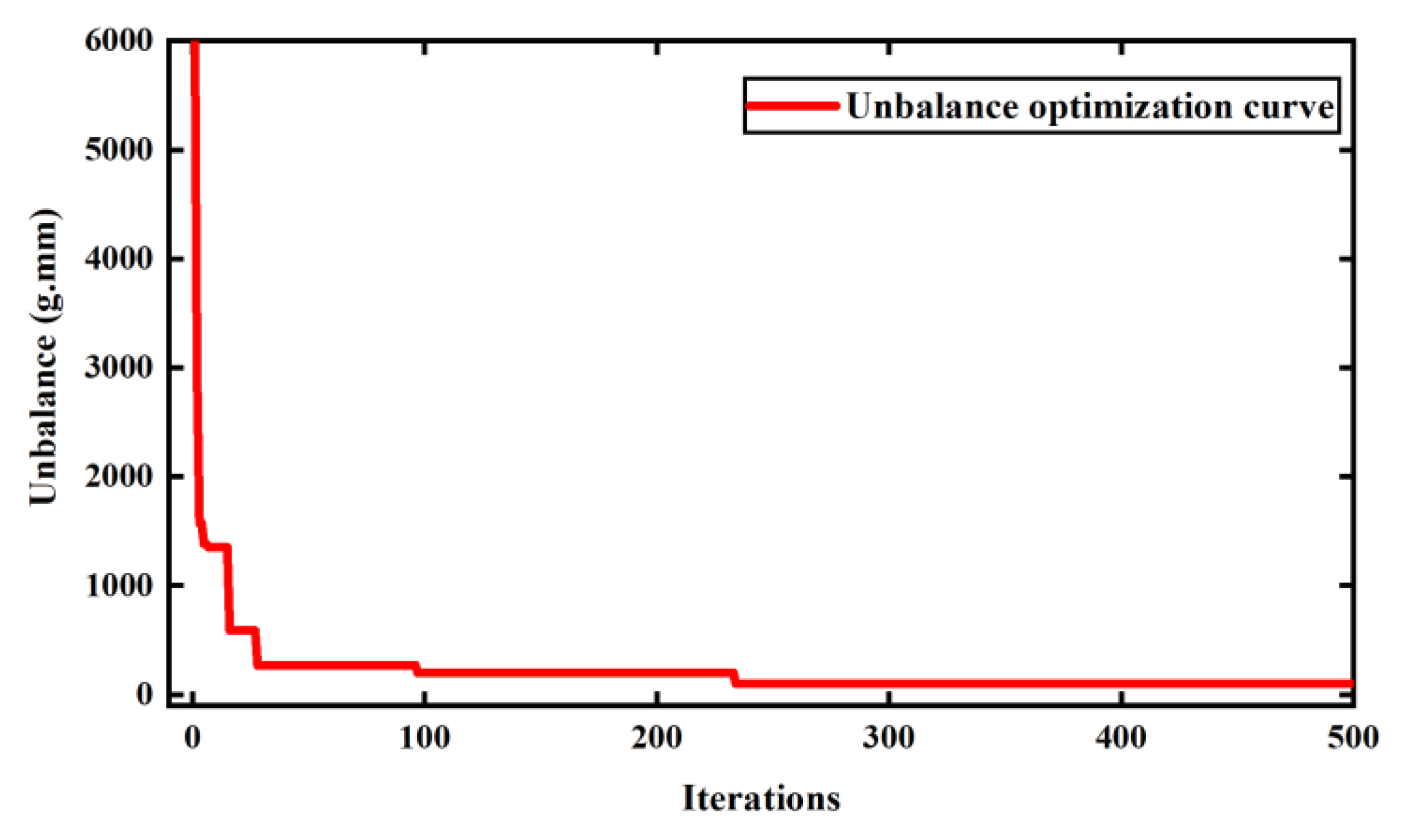
According to the mass moments given in Table 2, it was assumed that the disk unbalance is 0 g.mm. The cloud adaptive genetic algorithm was used to sort the blades. The set algorithm parameters were as follows: the population size N is 30; the maximum number of iterations is 500. The C sharp language was used to program the algorithm, and the algorithm was run on an ordinary PC with I7 2.4 GHz 4 GB running memory. It was found that the minimum unbalance of the population obtained varies with the number of iterations as shown in Figure 9.

According to Figure 9, we can see that when the number of iterations reaches 235, the maximum fitness result was achieved. For general or unreasonable sorting, the rotor unbalance amount can reach 6000 g.mm or more. As the number of iterations of the algorithm increases, the unbalance becomes smaller and smaller, until the minimum unbalance is 99.63 g.mm when the number of iterations reaches 235. The corresponding sorting result is shown in

Table 3. The result of blades sorting optimized by CAGA.

Assembly Location	Serial Number	Mass Moment (g.mm)	Assembly Location	Serial Number	Mass Moment (g.mm)
1	20	1,762,040	9	29	1,762,720
2	27	1,761,980	10	25	1,758,240
3	12	1,726,720	11	21	1,758,040
4	32	1,755,640	12	18	1,740,860
5	15	1,755,000	13	16	1,754,680
6	2	1,756,880	14	10	1,742,080
7	6	1,762,720	15	26	1,754,580
8	9	1,762,200	16	14	1,754,380
17	30	1,757,760	25	24	1,749,600
18	22	1,762,280	26	1	1,779,360
19	28	1,769,660	27	5	1,756,400
20	3	1,754,920	28	13	1,767,280
21	7	1,757,900	29	23	1,756,540
22	8	1,761,320	30	11	1,758,020
23	31	1,755,700	31	19	1,772,240
24	4	1,754,700	32	17	1,772,960

.

In order to compare the optimization effect of the cloud adaptive genetic algorithm, the blades were sorted according to several methods (weight sorted, sorting type 2, sorting-1/4 skip) mentioned in the paper [5], and the obtained unbalance sorting results are shown in Figure 10a–c. According to sorting type 2, this paper designed sorting type 4, that is, sorting type 2 was used to re-distribute the blades in four sectors, and the resulting unbalance sorting result is shown in Figure 10d. The unbalance sorting results obtained by the genetic algorithm (GA) and cloud adaptive genetic algorithm (CAGA) are shown in Figure 10e,f.

Figure 10 describes the assembly position of each blade and the arrangement of the mass moment under the six blade arrangement methods. These methods can obtain the unbalance value under several blade arrangements. Assuming that a mass block needs to be added to the circumference of a disk with a radius of 500 mm for the balancing process, the required balance mass is recorded in

Table 4. Unbalance under different assembly methods.

Assembly Method	Weight Sorted	Sorting Type 2	Sorting-1/4 Skip
Unbalance (g.mm)	10,039.8	7777.93	19,664.58
Balance mass (g)	200.080	15.556	39.329
Assembly method	Sorting Type 4	GA	CAGA
Unbalance (g.mm)	5390.11	2292.83	99.63
Balance mass (g)	10.780	4.586	0.199

.

It can be seen from Table 4 that the weight sorted method causes the largest unbalance in the assembly process. The sorting type 2, sorting type 4, and sorting-1/4 skip method reduce the unbalance after arrangement to a certain extent relative to the weight sorted. GA also optimized the unbalance to a certain extent, but it still cannot meet the requirement that the unbalance cannot be brought into the tolerance range from the process, and the mass of the corresponding mass that needs to be balanced does not meet the requirements. From the perspective of the balance method, the intelligent algorithm optimization effect is better than the empirical method. The unbalance of GA is at least 57.5% optimized relative to the first four methods, and the unbalance of the CAGA algorithm is optimized by 95.7% relative to GA.

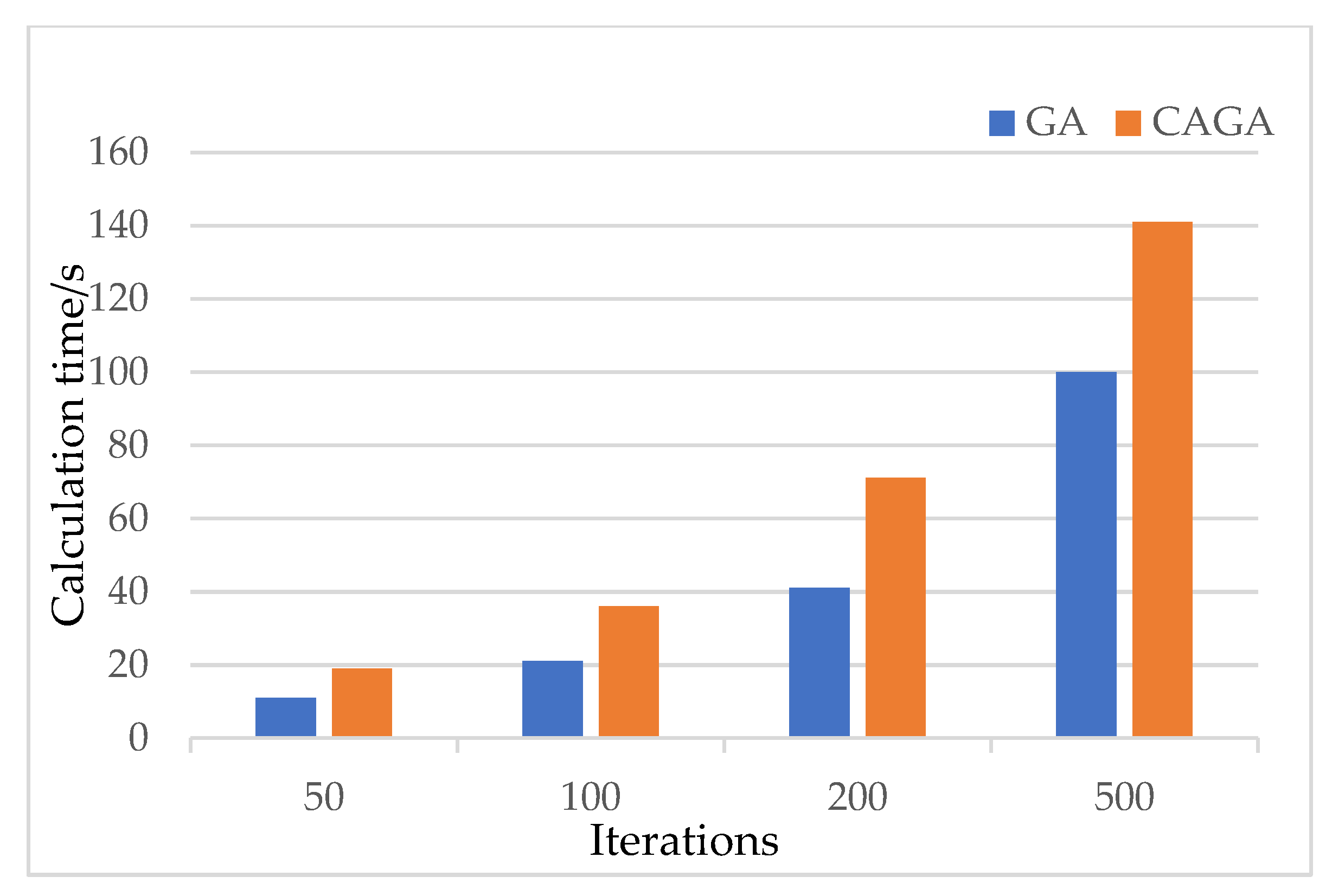
In order to check the accuracy and calculation time of the cloud adaptive genetic algorithm and genetic algorithm, the results of the two methods when the number of iterations are 50, 100, 200, and 500, respectively, are shown in Figure 11 and Figure 12.

Figure 11 shows that CAGA is much better than GA in terms of the algorithm accuracy, and the imbalance of the two methods decreases with the increase of the number of times. Figure 12 illustrates that CAGA is slower than GA in terms of the calculation time.

For the general blade sorting process, the initial unbalance of the disk is not considered. This approach reduces the unbalance of the blade sorting result, but due to the existence of the initial unbalance of the disk, the assembly unbalance after the sorting is not reduced. Therefore, the calculation results obtained by setting the disk unbalance in the X direction as 100, 200, and 500 g.mm in this paper are shown in

Table 5. Blade arrangement under different initial unbalance.

Disk Unbalance (g.mm)	Unbalance (g.mm)	Blades Unbalance/g.mm	Calculation Time (s)
0	99.63	99.63	70
100	101.87	152.7	74
200	5.75	194.6	71
500	51.76	458.04	72

.

It can be seen from Table 5 that at the same time, different initial unbalance can still get better results. When the unbalance amount is 200 g.mm, the unbalance amount after optimization even reaches 5.75 g.mm, which shows that the method is still effective for the optimization of blade sorting with the initial unbalance amount. The second and third columns of the table compare the final imbalance of the same blade sequence when the imbalance of Table 5 is included, and the imbalance of the blade is only considered when the optimal rotor imbalance is reached. It can be seen from the table that the model that considers the imbalance of the leaf disc is much smaller than the imbalance that only considers the residual error of the blade, which proves the effectiveness of the model.

5. Conclusions

The cloud adaptive genetic algorithm was used to sort rotor blades with eccentric disk-mass moment unbalance. The rotor mass moment model, the specific process of blade sorting by the genetic algorithm, and improvement of the crossover and mutation operators by the cloud adaptive genetic algorithm were introduced. The experimental results show that this method greatly reduces the asymmetry of the rotor mass moment, reduces the relative manual operation time and manpower, and optimizes the local optimization of the relative general genetic algorithm. However, the rotor mass moment unbalance cannot be eliminated generally. The minimum unbalance is related to the actual blade and disk mass moment unbalance as well as the blade distribution angle, so the blade sorting can only make the rotor mass moment meet the design requirements after sorting. This method provides a fast rotor moment balance method and can also be used to optimize the order of other unbalance blades.

References

- Kim, C.J. Location of unbalance mass and supporting bearing for different type of balance shaft module. Mech. Sci. 2018, 9, 259–266. [Google Scholar] [CrossRef]
- Prasad, V.; Tiwari, R. Identification of Speed-Dependent Active Magnetic Bearing Parameters and Rotor Balancing in High-Speed Rotor Systems. J. Dyn. Sys. Meas. Control 2019, 141, 041013. [Google Scholar] [CrossRef]
- Bhende, A.R. Dynamic balancing of a two-plane rotor without phase angle measurement using the amplitude subtraction method. Insight 2020, 62, 42–45. [Google Scholar] [CrossRef]
- Choi, W.; Storer, R.H. Heuristic algorithms for a turbine-blade-balancing problem. Comput. Oper. Res. 2004, 31, 1245–1258. [Google Scholar] [CrossRef]
- Piskin, A.; Aktas, H.E.; Topal, A.; Turan, O.; Baklacioglu, T. Rotor Balancing with Turbine Blade Assembly Using Ant Colony Optimization for Aero-Engine Applications. Int. J. Turbo. Jet Engines 2017. [Google Scholar] [CrossRef]
- Von Backström, T.; Du Buisson, J. Blade Arrangement Strategies for Minimal Rotor Unbalance. Int. J. Turbo. Jet Engines 1994, 11, 193–200. [Google Scholar] [CrossRef]
- Lavagnoli, S.; De Maesschalck, C.; Andreoli, V. Design Considerations for Tip Clearance Control and Measurement on a Turbine Rainbow Rotor with Multiple Blade Tip Geometries. J. Eng. Gas Turbines Power 2017, 139, 042603. [Google Scholar] [CrossRef]
- Amiouny, S.V.; Bartholdi, J.J.; Vate, J.H. Heuristics for Balancing Turbine Fans. Operations Research. Oper. Res. 1999, 48, 591–602. [Google Scholar] [CrossRef] [Green Version]
- Pitsoulis, L.S.; Pardalos, P.M.; Hearn, D.W. Approximate solutions to the turbine balancing problem. Eur. J. Oper. Res. 2001, 130, 147–155. [Google Scholar] [CrossRef]
- Li, D.D.; Chen, Y.; Yu, D.R. Research of optimizing arrangement for turbine blade installation based on ant colony algorithm. J. Cent. South Univ. 2011, 42, 187–191. [Google Scholar]
- Zhao, T.; Yuan, H.; Yang, W. Genetic particle swarm parallel algorithm analysis of optimization arrangement on mistuned blades. Eng. Optimiz. 2017, 49, 2095–2116. [Google Scholar] [CrossRef]
- Mason, A.; Rönnqvist, M. Solution methods for the balancing of jet turbines. Comput. Oper. Res. 1997, 24, 153–167. [Google Scholar] [CrossRef]
- Thompson, E.; Becus, G. Optimization of blade arrangement in a randomly mistuned cascade using simulated annealing. Aerospase Eng. Eng. Mech. 1993, 10, 1993–2254. [Google Scholar] [CrossRef]
- Wen, Z.; Wei, G. Optimal blade placement for large turbofan balancing. In Proceedings of the Fourth International Conference on Computer Integrated Manufacturing and Automation Technology, Troy, NY, USA, 10–12 October 1994; pp. 261–266. [Google Scholar] [CrossRef]
- Yuan, H.; Zhao, T.; Yang, W. Annealing evolutionary parallel algorithm analysis of optimization arrangement on mistuned blades with non-linear friction. J. Vibro Eng. 2015, 17, 4078–4095. [Google Scholar]
- Yiping, D.; Cai, J.; Shi, L. Development and Application of Blades Installation Arrangement Order Optimizing System Based on Genetic Algorithm. Turbine Technol. 2003, 5, 270–272. [Google Scholar]
- Mao, L.R.; He, B.; An, Y.; Fu, J.; Fan, Q.S. Research of Small Wind Turbine Blades Matching Optimization Technology. Mach. Des. Manuf. 2012, 10, 99–101. [Google Scholar]
- Er-Ming, H.E.; Geng, Y.; Li, H.E. Application of Genetic Algorithm in Blade Arrangement of Engine. Mech. Sci. Technol. 2003, 4, 553–555. [Google Scholar]
- Pan, W.; Zhang, M.; Tang, G. Blade Arrangement Optimization FOR Mistuned Bladed Disk Based on Gaussian Process Regression and Genetic Algorithm. J. Eng. Gas. Turbines Power Trans. 2020, 142, 021008. [Google Scholar] [CrossRef]
- Zhao, L.; Li, B.; Chen, H.; Yao, Y. An assembly sequence optimization oriented small world networks genetic algorithm and case study. Assem. Autom. 2018, 38, 387–397. [Google Scholar] [CrossRef]
- Li, Y.; Yuan, H.; Yang, S. Optimization on Mistuning Blades Arrangement of Vibration Absorption Based on Genetic Particle Swarm Algorithm in Aero-Engine. Adv. Mater. Res. 2013, 655-657, 481–485. [Google Scholar] [CrossRef]
- Wang, L.; Luo, W.Y. Improved non-dominated sorting genetic algorithm (NSGA)-II in multi-objective optimization studies of wind turbine blades. Appl. Math. Mech. Engl. Ed. 2011, 32, 739–748. [Google Scholar] [CrossRef]
- Holland, J.H. Adaptation in Natural and Artificial Systems: An Introductory Analysis with Applications to Biology, Control, and Artificial Intelligence; MIT Press: Cambridge, UK, 1992. [Google Scholar] [CrossRef]
- Dai, C.H.; Zhu, Y.F.; Chen, W.R. Adaptive genetic algorithm based on cloud theory. Control Theory Appl. 2007, 4, 646–650. [Google Scholar]
Figure 1.
Random blade sorting model.
Figure 2.
Optimum blade sorting of the torque minimization model.
Figure 3.
Sum of the torque vectors of random blade sorting.
Figure 4.
Vector sum of the torque minimization model.
Figure 5.
Vector sum model of the mass moment both the random sorting blades and disk.
Figure 6.
Vector sum model of the mass moment both the optimum sorting blades and disk.
Figure 7.
Basic flow chart of the genetic algorithm.
Figure 8.
Rotor test piece composed of blades and disk.
Figure 9.
CAGA optimization process.
Figure 10.
The mass moment arrangement of the blades under the 6 arrangement methods: (a) Weight sorted; (b) Sorting Type 2; (c) Sorting-1/4 skip; (d) Sorting Type 4; (e) GA; (f) CAGA.
Figure 11.
GA and CAGA optimization accuracy comparison.
Figure 12.
Comparison of the GA and CAGA calculation time.