
Calculation of the Statistical Properties in Intermittency Using the Natural Invariant Density


1
Departamento de Aeronáutica, Instituto de Estudios Avanzados en Ingeniería y Tecnología (IDIT), FCEFyN, Universidad Nacional de Córdoba and CONICET, Córdoba 5000, Argentina
2
Departamento de Física Aplicada, ETSIAE, Universidad Politécnica de Madrid, 28040 Madrid, Spain
3
Instituto de Estudios Avanzados en Ingeniería y Tecnología (IDIT), Universidad Nacional de Córdoba and CONICET, Córdoba 5000, Argentina
*
Author to whom correspondence should be addressed.
Symmetry 2021, 13(6), 935; https://0-doi-org.brum.beds.ac.uk/10.3390/sym13060935
Submission received: 30 March 2021
/
Revised: 14 May 2021
/
Accepted: 20 May 2021
/
Published: 25 May 2021
(This article belongs to the Special Issue Topological Field Theory and Stochastic Dynamics)
Abstract
:We use the natural invariant density of the map and the Perron–Frobenius operator to analytically evaluate the statistical properties for chaotic intermittency. This study can be understood as an improvement of the previous ones because it does not introduce assumptions about the reinjection probability density function in the laminar interval or the map density at pre-reinjection points. To validate the new theoretical equations, we study a symmetric map and a non-symmetric one. The cusp map has symmetry about , but the Manneville map has no symmetry. We carry out several comparisons between the theoretical equations here presented, the M function methodology, the classical theory of intermittency, and numerical data. The new theoretical equations show more accuracy than those calculated with other techniques.
1. Introduction
In chaotic intermittency, the solutions of the dynamical systems exhibit the alternation between chaotic and laminar behaviors. The laminar phases, also called regular phases, are related to pseudo-equilibrium regions or pseudo-periodic solutions. The bursts correspond to chaotic behavior [1,2,3,4]. Intermittency has been observed in engineering, physics, medicine, chemistry, and economy [5,6,7,8,9,10,11,12,13,14]. In addition, intermittency has been associated with the symmetry breaking in chaotic and stochastic systems [15,16]. Therefore, a more complete and accurate description of the intermittency phenomenon would be applied in several subjects. In the classic theory, intermittency was classified into three types, I, II and III, and later, other types were introduced [17,18,19,20,21,22,23].
One-dimensional maps are widely used to study chaotic intermittency [1,2,3,4]. These maps have a mechanism to reinject the trajectories from the chaotic region to the laminar one, which determines the reinjection probability density (RPD) function [1,3]. The RPD function describes the probability of the trajectories to be reinjected at each point of the laminar interval. Usually, once the RPD is calculated, other statistical functions can be obtained as the probability density of the laminar lengths (PDLLs), the characteristic relation, etc. The reinjection process can be very complex as indicated in [24]. Accordingly, an accurate calculation of the RPD function and other statistical properties is essential to explain the intermittency phenomenon.
We note that there was not a general methodology to obtain the RPD, and distinct schemes were utilized. The classical theory of intermittency considers a uniform RPD function. This assumption generates the classic characteristic relations, which establish how the average laminar length tends to infinity as a control parameter tends to zero [1,2,25]. A more general RPD has been introduced in the last few years. Accordingly, the characteristic relations were generalized too. To calculate this general RPD, the M function methodology was developed, which has worked accurately for maps with types I, II, III and V intermittencies without and with noise. The M function methodology uses a less restrictive assumption of a constant density at points that govern the reinjection process, i.e., pre-reinjection points [3,26,27,28,29,30,31,32,33,34,35].
In this paper, we introduce a new methodology to evaluate the RPD function, , and other statistical properties. We call it the density technique. To develop this technique, we use the Perron–Frobenius operator and the invariant density of the map. This study does not introduce assumptions about the RPD in the laminar interval, as does the classical theory, or the map density at pre-reinjection points, as does the M function methodology, because it uses the invariant density of the map. To validate the new theoretical equations, we analyze the cusp map [36,37] and the classical Manneville map [4,38]. The cusp map is symmetric about the axis , and the Manneville map has no geometric symmetry. Therefore, we study the new methodology in symmetric and non-symmetric maps. We carry out several comparisons between the theoretical results here presented, the classical theory of intermittency, the M function methodology, and numerical data.
2. The Perron–Frobenius Operator
The Perron–Frobenius operator is used here to transform random variables. Therefore, we briefly describe this operator. A more complete explanation about the Perron–Frobenius operator can be found in [37,39].
Let us study a family of evolution operators , such as identity and , where is a compact manifold, , and t is the evolution variable. If t takes only discrete values, the operator is a map. There are, at least, two formulations to describe the behavior of . One formulation corresponds to study the evolution of individual trajectories, the other one considers the evolution of the trajectories’ density.
For , the Perron–Frobenius operator evaluates the evolution of the trajectories’ density. We analyze a map , which transforms some interval in another interval . Then, and . In , the density of trajectories is , while in the trajectories’ density is . The Perron–Frobenius operator, , evaluates the density from , and we write . If , where y is variable, the Perron–Frobenius operator calculates the density
Note that Equation (1) supposes that is differentiable and invertible with continuous [39]. On the other hand, the theoretical formulation of the M function methodology requires that exists [3,30].
Let us now introduce a map , which is piecewise differentiable and satisfies , except in a finite number of critical points. Suppose that is an interval containing no critical values, and suppose that is the union of finitely many intervals, , each of which is mapped monotonically onto , then the Perron-Frobenius operator allows us to evaluate the density evolution:
where z is the number of intervals.
3. Evaluation of Statistical Properties
In this section, we calculate several functions and parameters to describe chaotic intermittency. First, we study the RPD function, then we analyze other statistical properties: the PDLL function, the characteristic relation, the intermittency factor, the number of iterations in the laminar and non-laminar phases, and the number of times that a trajectory crosses the boundary between laminar and non-laminar zones.
3.1. Evaluation of the RPD
The probability measure in an interval S can be written as
where is the characteristic function of the interval S
Therefore, the probability measure shows the frequency that the trajectory reaches the interval. We can relate the invariant density, , with the probability measure, , by
Now, we divide the whole data series into three subsets
First, we select and in the preceding iteration it has already been there, that is and . For the next one, we have but in the preceding period it has not been there, that is and . Finally, . Note that there is no intersection between them.
Therefore, the probability measure can be written as
The first term in the RHS is the probability for the trajectory to be in S when in the previous iteration it has been there. If (where is the laminar interval), then, only the second term in the RHS determines the RPD function, , through the relation
The weight w is included because it is current to normalize the RPD function over the laminar interval as . Therefore, to obtain the RPD function, the sum in Equation (2) must exclude the contributions that do not generate reinjection in the laminar zone [3,40]
where l indicates the intervals that do not generate reinjection and is the density in the preceding iteration to reinjection. The weight w can be calculated from the normalization condition:
We can organize the intervals following
Therefore, Equation (2) can be written as
If the map has an invariant density, , it verifies . Then, Equation (13) becomes
Using Equations (10) and (14), the RPD function can be calculated by two alternative equations. The first one is
and the second one results
Equation (15) calculates the RPD from points outside the laminar interval that are reinjected inside it, i.e., points that verify and . In contrast, Equation (16) evaluates the RPD function by subtracting from the invariant density points that were in the laminar interval at the previous iteration and that remain in it, i.e., points that verify and . Finally, the RPD function must satisfy the normalization condition given by Equation (11).
3.2. Evaluation of Other Statistical Properties
For each reinjected point x, there is a laminar length , which determines the number of iterations that the trajectory needs to move from x to the boundary of the laminar interval c. Thus, the PDLL function establishes the probability of finding laminar intervals of length l. Usually, the PDLL function is obtained from the RPD function as follows [1,3]
Here, we evaluate the PDLL function using the invariant density of the map without calculating previously the RPD function. If we introduce Equation (15) in Equation (17), we obtain
where x represents the pre-reinjection points, and . From the last equation, we calculate the probability density of the laminar lengths directly from the invariant density of the map.
In addition, the characteristic relation, , can be calculated from the invariant density
where L is the average laminar length.
Directly from the invariant density, we can determine the “time” that the trajectory spends in laminar and non-laminar behaviors. Let us consider a process with iterations. Where and are the numbers of iterations inside and outside of the laminar interval, respectively,
is the interval where the map is defined, and there is no intersection between and : . The relation between them is
Note that , where is the parameter controlling the route from regular to chaotic behavior.
From the previous relation, we can obtain the average non-laminar length, C
where the average laminar length, L, is given by Equation (19).
The intermittency factor, , determines the probability that a trajectory is outside the laminar interval. It can be calculated from the invariant density as
Finally, the number of times a trajectory crosses the boundary between the laminar and non-laminar interval results
Note that and also depend on .
For a map with intermittency, Equations (18)–(24) allow us to directly calculate the probability density of the laminar lengths, the average laminar and non-laminar lengths, the characteristic relation, the number of iterations in laminar and non-laminar phases, the intermittency factor, and the number of crosses between the laminar and non-laminar zones without the evaluation of the reinjection probability density function.
4. Application to the Cusp Map
Let us introduce the following map:
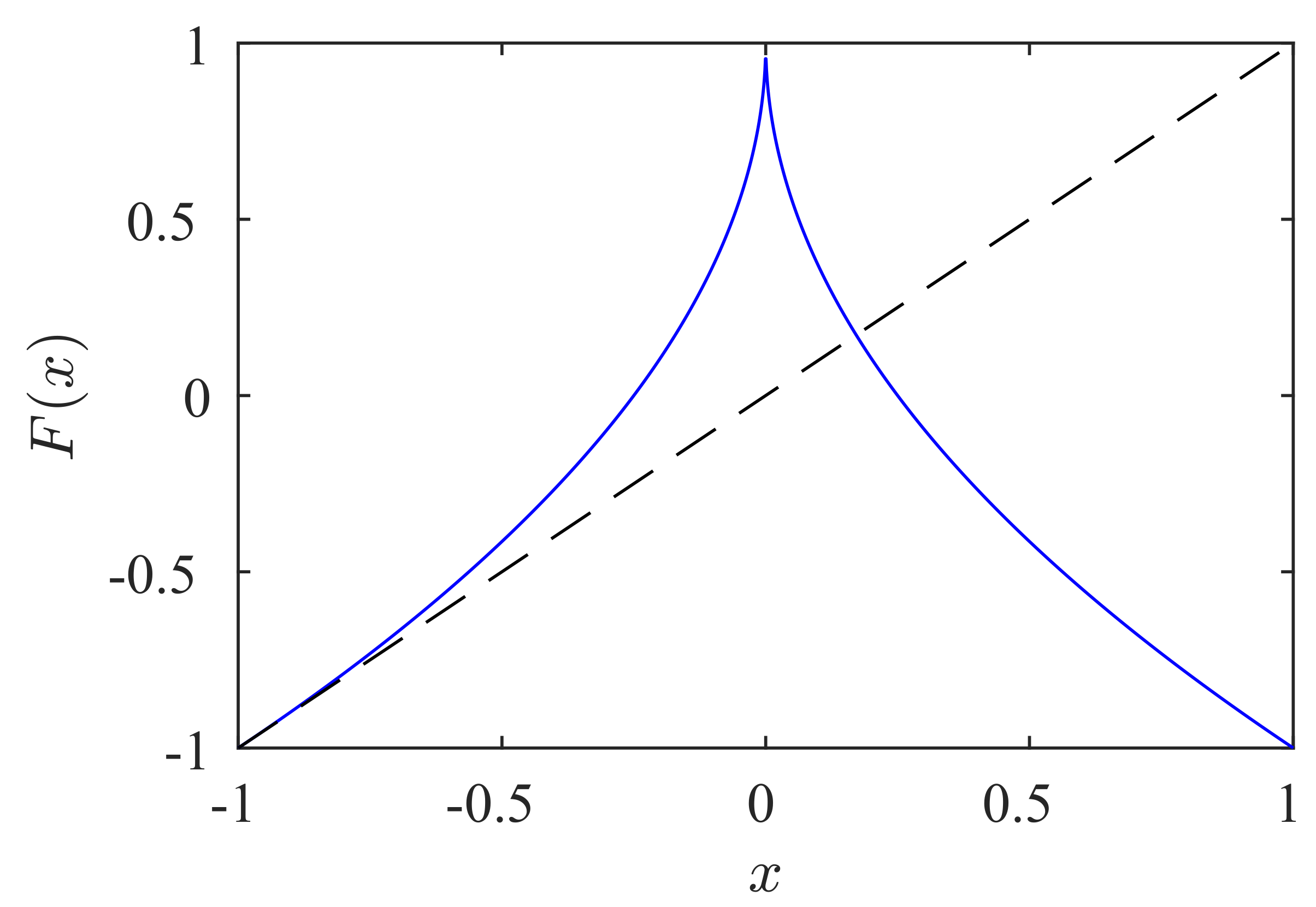
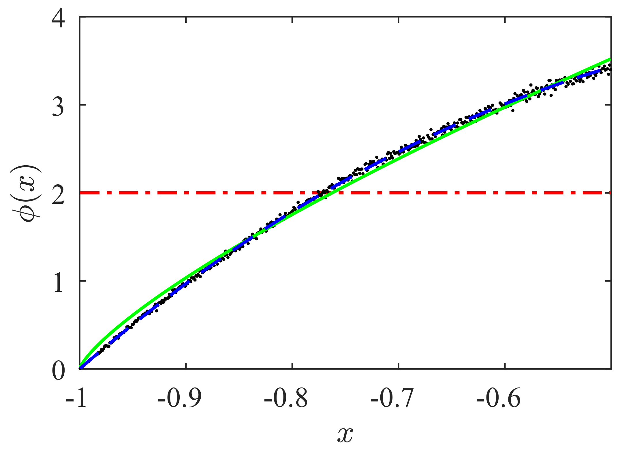
Note that for , the cusp map is recovering [36,37]. For , the map has a fixed point at , which disappears for , and for type-I intermittency occurs. Figure 1 shows the map given by Equation (25) for . Note that the cusp map given by Equation (25) has symmetry about .
The cusp map has an invariant density [37]
For the map (25), the number of intervals is , and , . In accordance with Equation (15), the RPD function results
and using Equation (16), the RPD function can be calculated as
if , is defined as
and
The derivative is
Then, from Equations (26), (27) or (28) and (31), the RPD can be obtained
where w is calculated from the normalization condition, Equation (11)
is the fixed point, and c is the semi-amplitude of the laminar interval, .
Results
To validate the previous theoretical equations, we perform the comparison between the RPD function given by Equation (32) with those calculated by the M function methodology, the classical theory, and with numerical data. A detailed explanation of the M function methodology can be found in Refs. [3,29,30,31,32,33,34,35]. The RPD calculated using the M function methodology results
To evaluate the Equation (34), we use the function defined as
where for all reinjected points x. Note that the function can be calculated as the average of reinjection points in the interval , then, if we arrange the reinjections following the relation , a very simple evaluation of the function can be obtained
We emphasize that Equation (36) does not need to know the function . For the RPD given by Equation (34), is a linear function
where in Equation (34) is obtained from the slope m
On the other hand, the classical theory of intermittency assumes uniform reinjection, . Note that the classical theory is only a particular case of Equation (34) for ().
We emphasize that, to obtain Equation (34), the assumption of constant density at pre-reinjection points was introduced (see [3,30]).
To calculate the numerical data, we generate an iterative process for the map given by Equation (25); also, we divide the laminar interval into sub-intervals, then we calculate the histogram of reinjections and the numerical RPD function. To obtain the histogram, we consider at least reinjections, which implies millions of iterations.
We develop several numerical tests for a different number of reinjected points N, and we split the laminar interval into sub-intervals where the RPD functions are evaluated. To study the convergence process of the theoretical RPD functions given by Equations (32) and (34) and the classical theory of intermittency regarding the numerical data, we evaluate
where and are the theoretical and numerical values of the RPD in the sub-interval j.
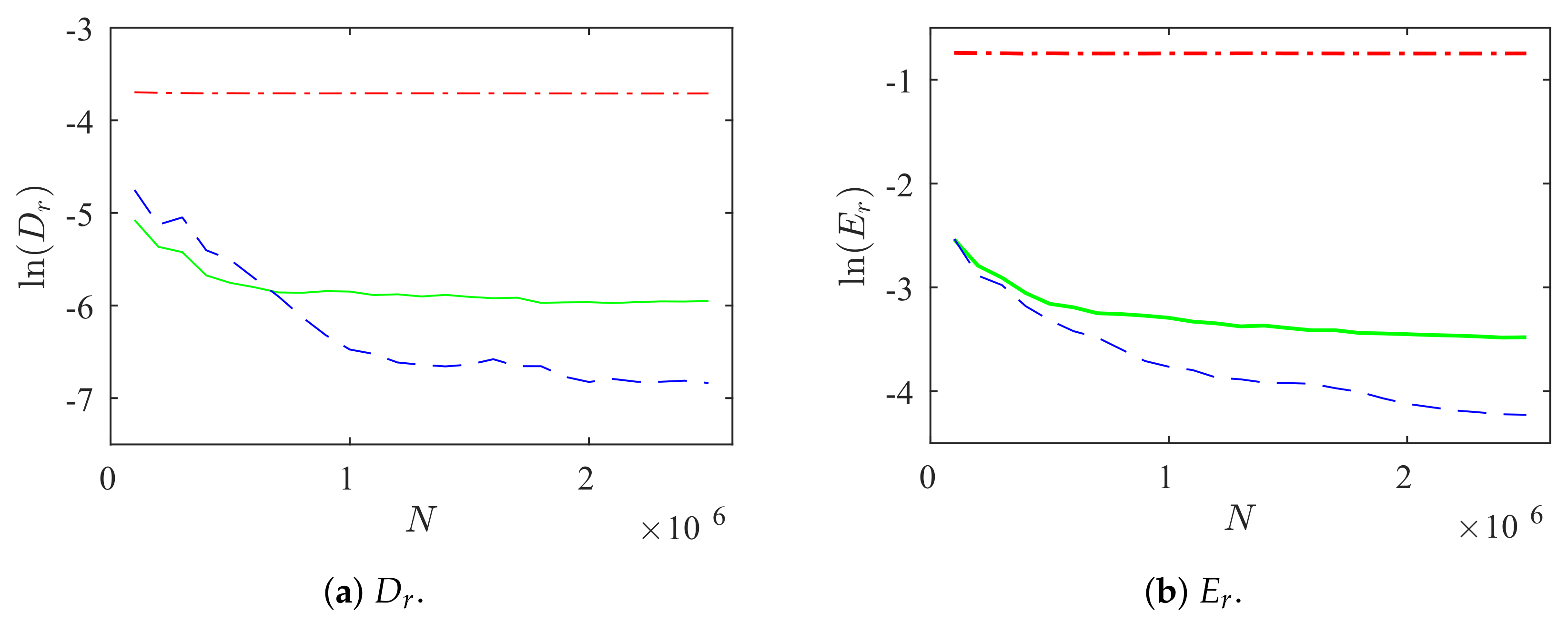
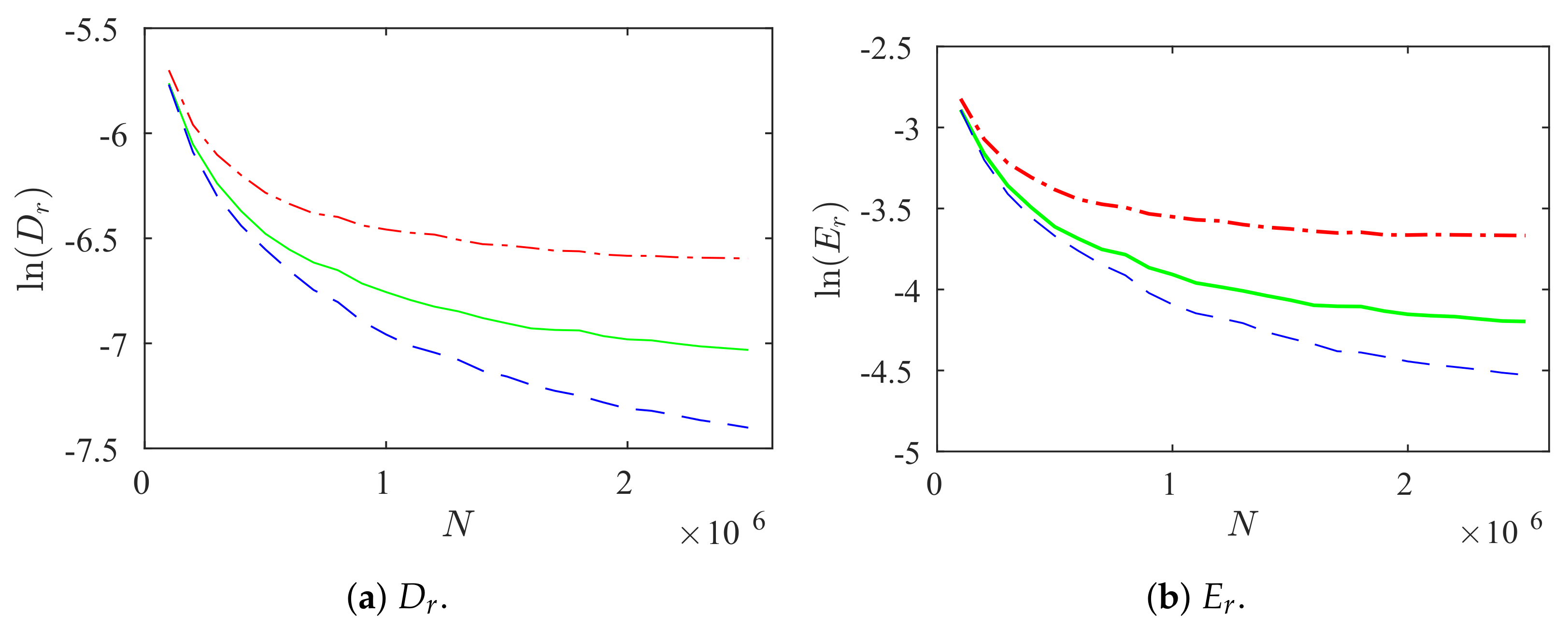
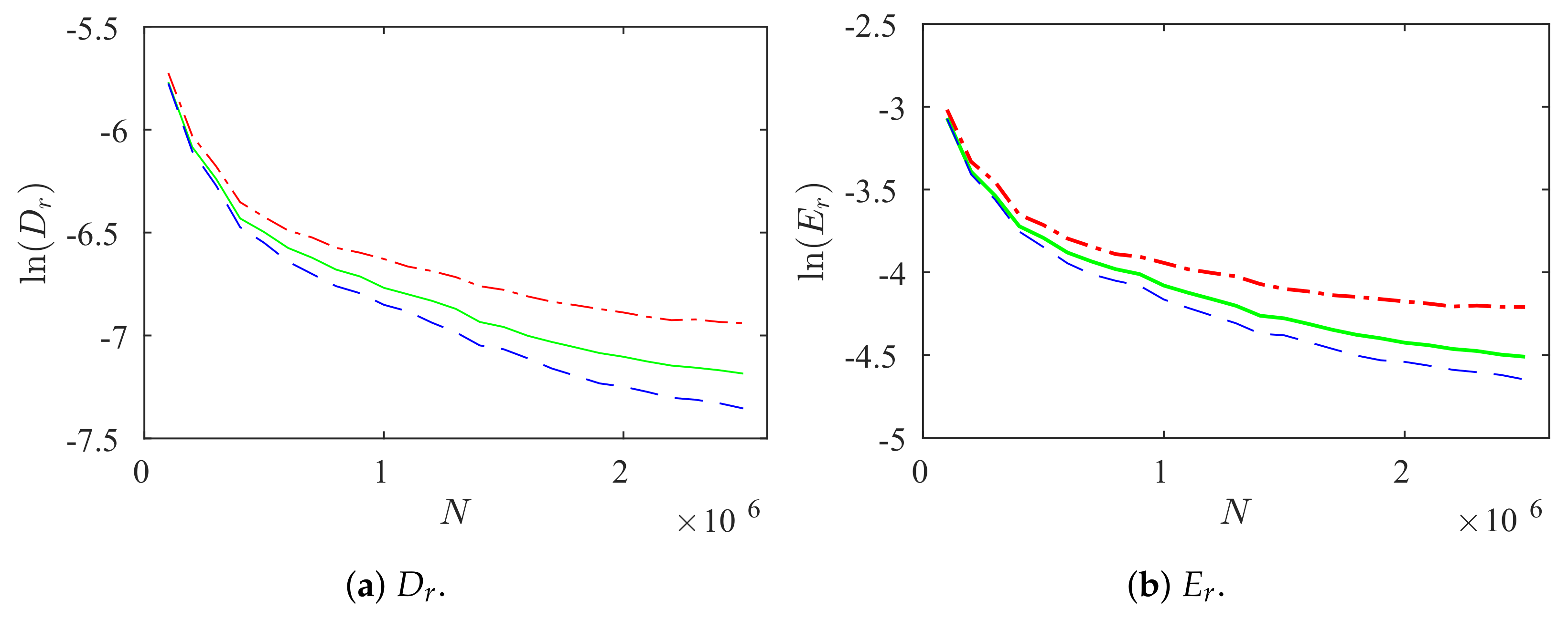
We study two sets of tests. For the first one, we consider the following parameters , , and . Figure 2a,b show and respectively, for different numbers of reinjected points, N from 100,000 to 2,500,000. We emphasize that as the number of reinjected points increases, the accuracy of the density technique and the M function methodology increases too. In addition, we note that the errors generated by Equation (32) are lower than those obtained from Equation (34). On the other hand, the M function methodology obtains . Theoretical and numerical RPDs are shown in Figure 3, the black points are the numerical data, the blue, green, and red lines are the RPD functions given by Equations (32) and (34) and the classical theory, respectively. From Figure 2a,b and Figure 3, we can observe the convergence and accuracy of the theoretical formulation here presented.
To calculate the rate of convergence of the results, we utilize the sequence that tends to zero when N tends to infinite, and we must verify
where , , and are positive real numbers. Then, we can say that and converge to zero with rate, or order, of convergence and , respectively [41]. For this test, we find that and . Therefore, and converge to zero when N tends to infinity.
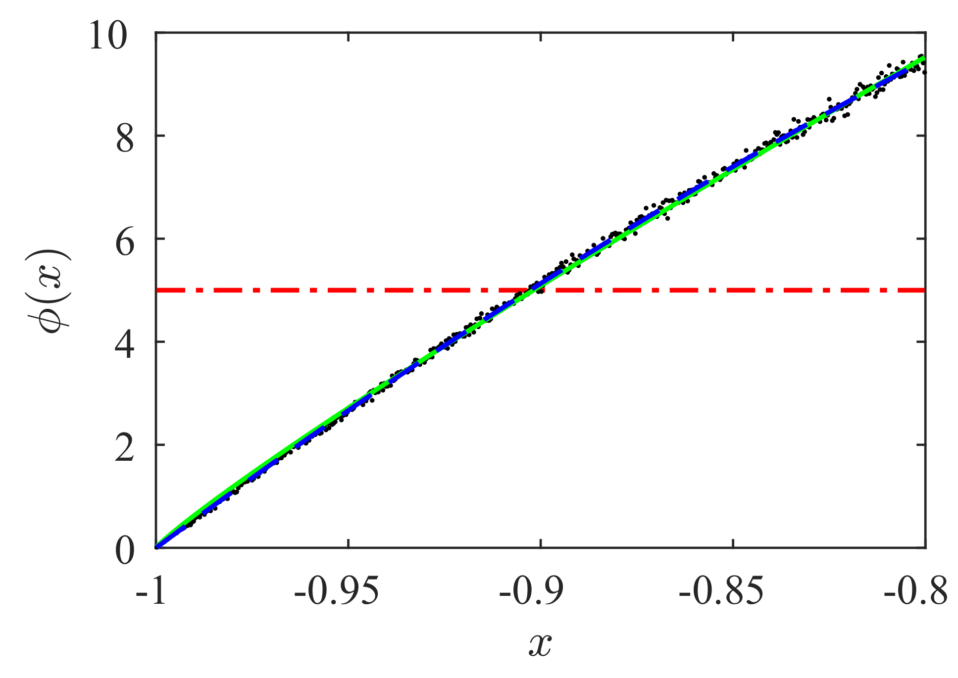
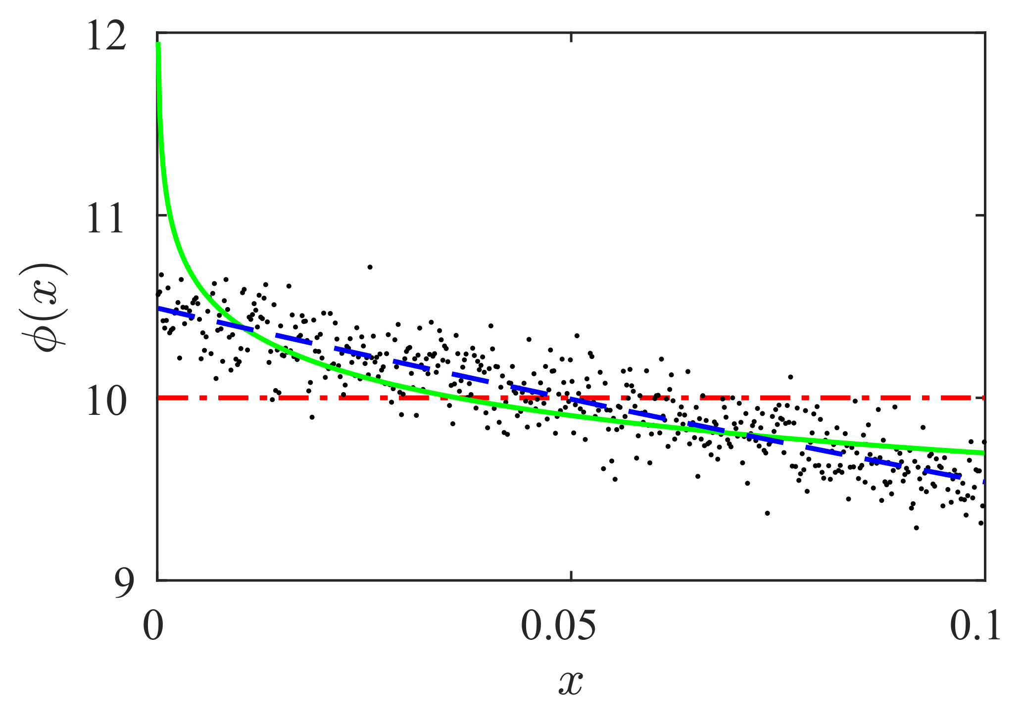
The second set of tests uses the following parameters , , and . Figure 4a,b show and , respectively, for N = 100,000–2,500,000. Similar to the previous tests, as the number of reinjected points increases the accuracy of RPD calculated by the M function and the new theoretical formulation increases too. Again, the classical theory has the worst behavior. Additionally, we note that the errors generated by Equation (32) are lower than those obtained from Equation (34). As in the previous set of tests, the M function methodology obtains . Theoretical and numerical RPDs are shown in Figure 5, the black points are the numerical data, the blue, green, and red lines are the RPD functions given by Equations (32) and (34) and the classical theory, respectively.
If we apply Equation (40) for the density technique, we obtain , then and converge to zero for .
5. Application to the Manneville Map
The following map
is the classical map introduced by Manneville [4]. For this map, is a stable fixed point for , and for , the point loses its stability and type II intermittency occurs. The map is shown in Figure 6 for . We highlight that the Manneville map given by Equation (41) has no geometric symmetry.
The invariant density for this map was deduced in [42]
we have introduced K to normalize the density inside the interval
The number of intervals is , with , and . From Equation (15), the RPD function can be obtained as:
The points inside the interval are
where and .
The density is written in function of y as
and
From these last equations and the normalization condition, we obtain
Results
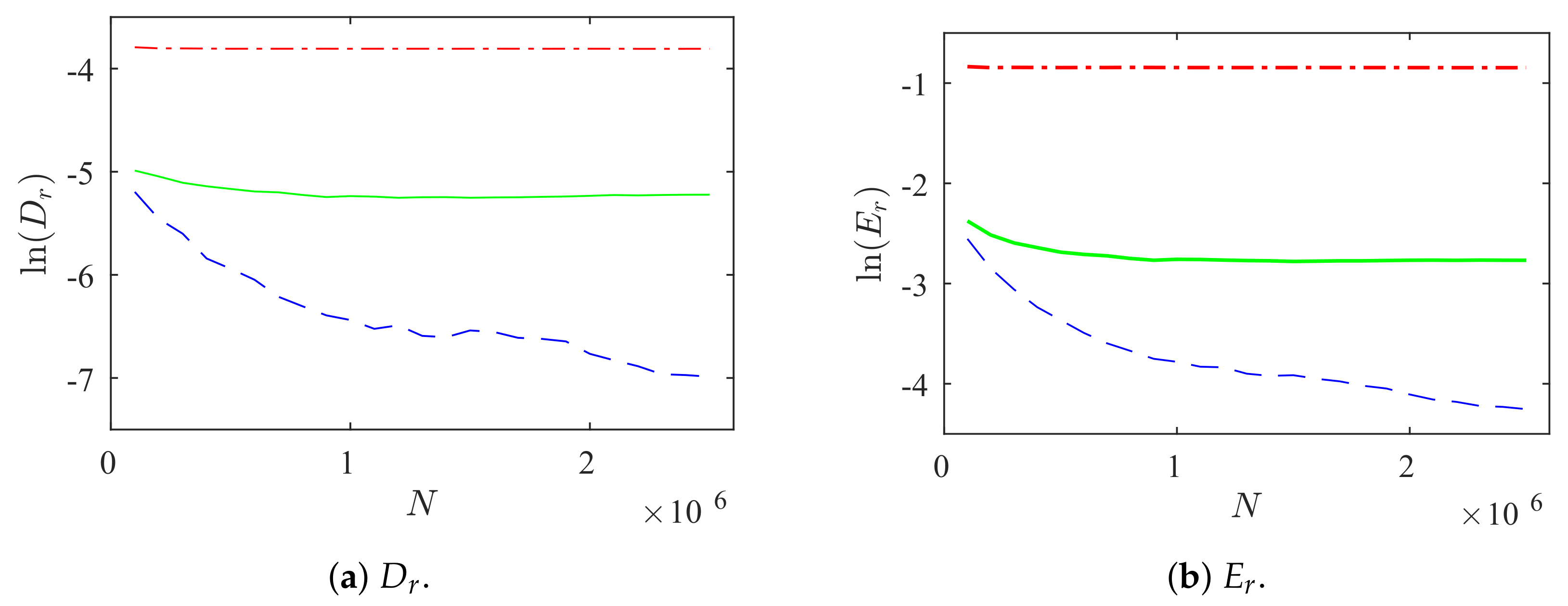
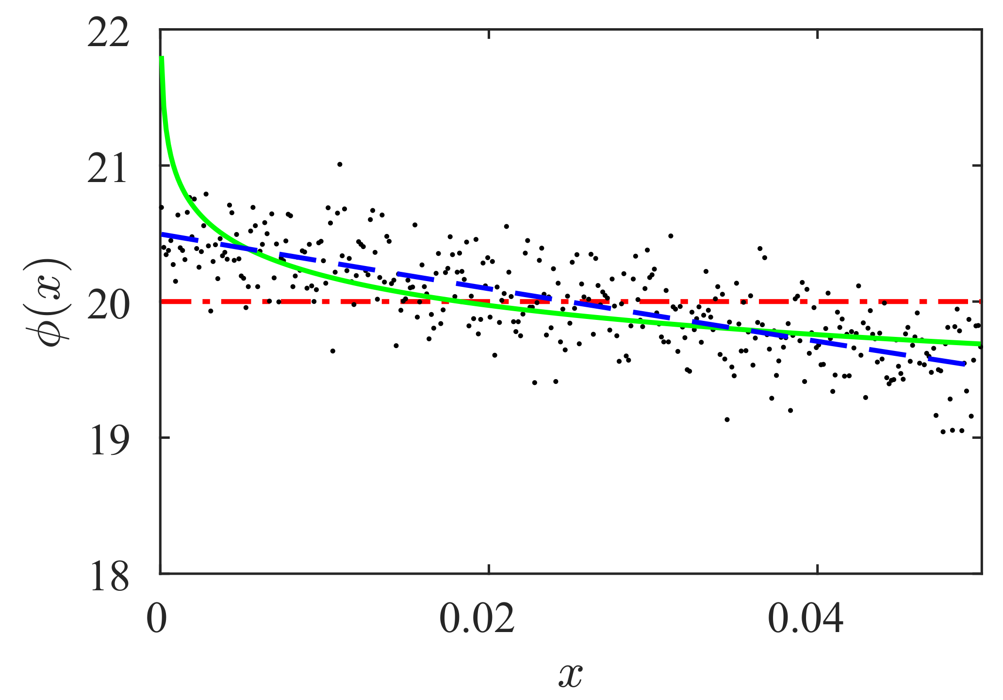
We present some numerical and theoretical results for the Manneville map (Equation (41)). We study two sets of tests with different parameters. The first set uses , , N = 100,000–2,500,000 and . The results are shown in Figure 7a,b and Figure 8. Figure 7a,b show the evolution of and vs. N. The results evaluated by the density technique are the dashed blue line, the green line corresponds to the M function methodology, and the red line to the classical theory. From these figures, we observe that the density technique approximates more accurately the RPD than the M function methodology and the classical theory. Figure 8 shows the RPD functions, the blue line is the RPD calculated by the density technique (Equation (48)), the green line is the RPD obtained by M function methodology (Equation (34)), the red line represents the classical RPD, and the black points are the numerical data. We note that the theoretical RPD calculated by Equation (48) captures accurately the numerical data. In addition, we emphasize that the RPD is approximately constant.
To evaluate the rate of convergence of these results, we use the Equation (40). For this set of tests, we obtain and . Then, and converge to zero when N tends to infinity with a rate of convergence and , respectively.
For this test, with = 500,000,000, we also calculate , , , C, , and . The comparison between numerical and theoretical results is shown in Table 1. The first file has the theoretical values calculated using Equations (18)–(24), the second file shows the numerical data, and the third one contains the percentage error
where and are the theoretical and numerical values, respectively.
From Table 1, good accuracy can be observed between theoretical results and numerical data.
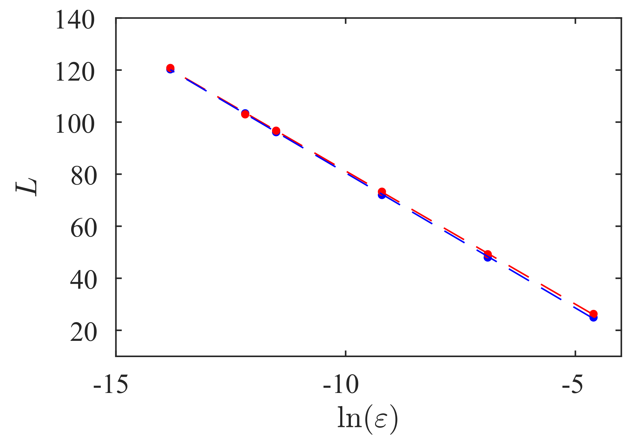
Using Equation (19), we calculate the characteristic relation for . Figure 9 shows the numerical (red points) and theoretical (blue points) results. Note that the characteristic relation can be written as
The dashed red and blue lines are the linear interpolation for the numerical and theoretical data with and , respectively. Note that . Therefore, the characteristic relation verifies .
Note that for , Equation (48) can be approximated in the laminar interval by a constant function
For an RPD that satisfies the last equation, the characteristic relation is given by Equation (50) with (see Ref. [38]).
For the second set, we use the following parameters, , , N = 100,000–2,500,000 and . Figure 10a,b and Figure 11 show the results. The evolution of and for different N is shown in Figure 10a,b. The blue, green, and red lines correspond to the density technique, the M function methodology, and the classical theory, respectively. The best results are obtained for the density technique. Figure 11 shows the RPD functions, the blue, green and, red lines are the RPDs calculated by the density technique (Equation (48)), the M function methodology (Equation (34)), and the classical theory, respectively, the black points are the numerical data. The theoretical RPD calculated by density technique captures accurately the numerical data.
The rate of convergence of these results is evaluated by Equation (40). We obtain . Accordingly, for with a rate of convergence .
We observe that the better results are calculated using the density technique here introduced.
In addition, we calculate with = 500,000,000 the following variables: , , , C, , and . The comparison between numerical and theoretical results is shown in Table 2. The first, second, and third files show the theoretical values calculated using Equations (18)–(24), the numerical data, and the percentage error given by Equation (49), respectively.
From Table 2, high accuracy can be observed between calculated numerical and theoretical results.
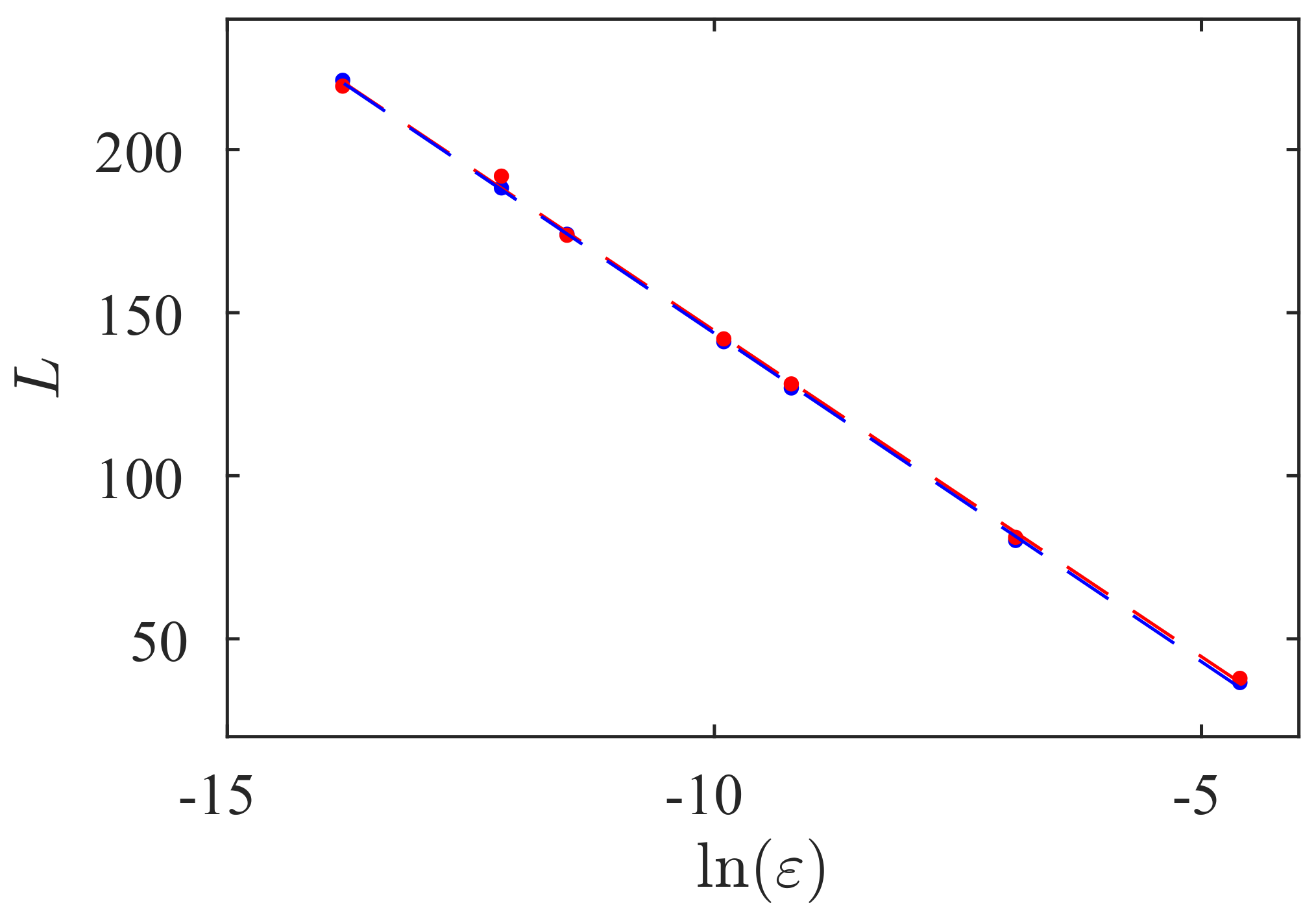
We evaluate, using Equation (19), the characteristic relation for . Figure 12 shows the numerical (red points) and theoretical (blue points) results. The red and blue dashed lines are the linear interpolations of the numerical and theoretical data, respectively. The characteristic relation calculated by the numerical data can be approximated by (red dashed line)
and the characteristic relation evaluated using theoretical results is (blue dashed line)
Note that both equations verify the characteristic relation given by Equation (50) with .
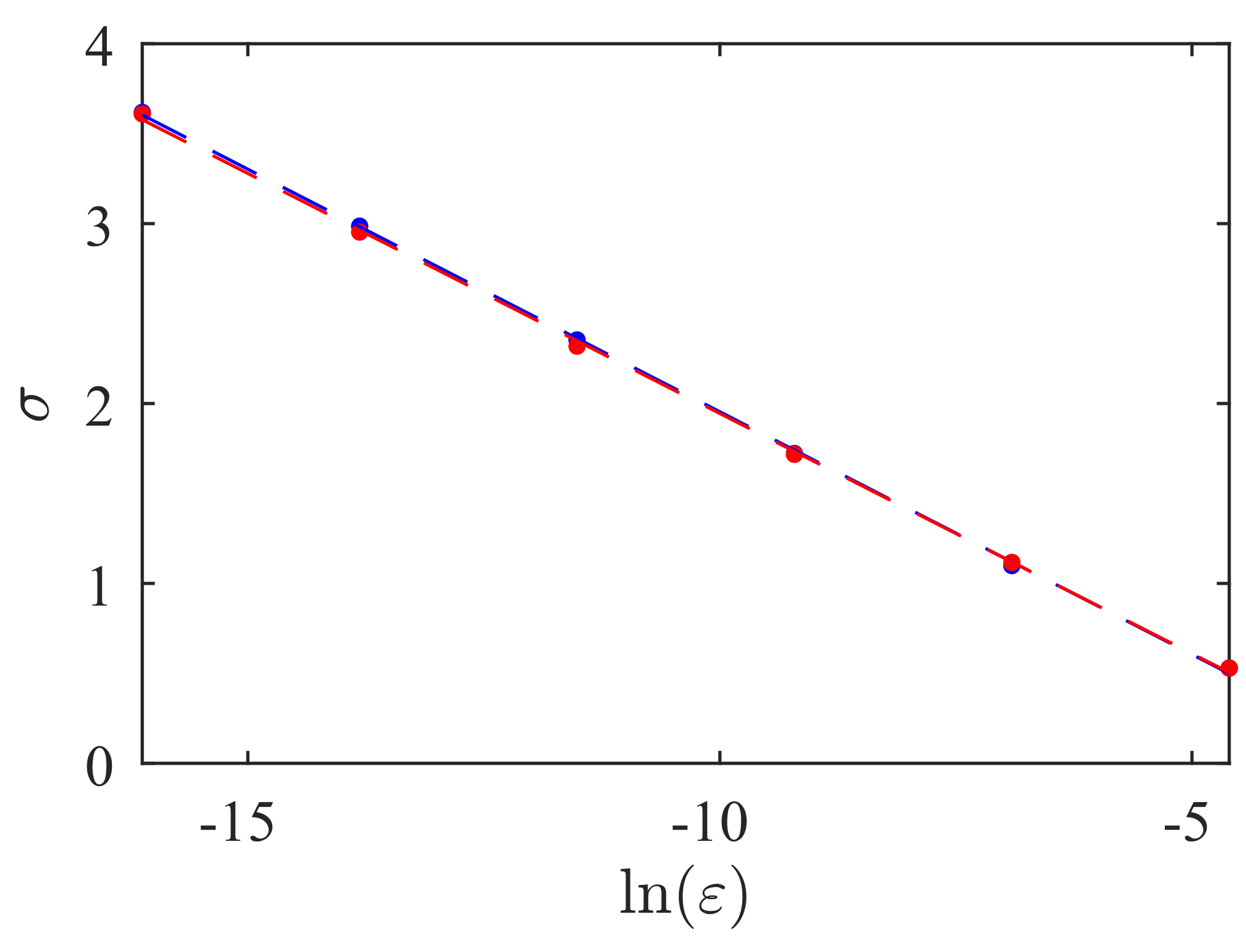
The relation between the number of iterations in laminar and non-laminar phases, , can be calculated. Figure 13 shows this relation. We observe that has a linear variation with . Remember that , where L has a linear dependence on , and ; therefore, C is also a linear function of , which implies that is a linear function with . increases as decreases, that is, the trajectory spends more time in the laminar zone for lower . From the figure, we note high accuracy between the numerical and theoretical results.
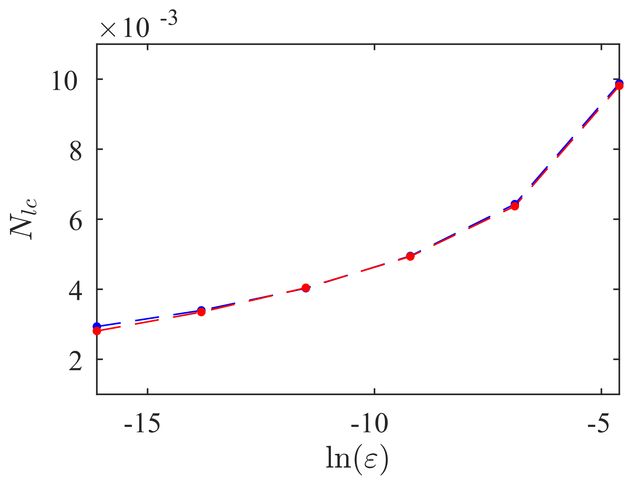
Finally, we calculate the number of crosses between the laminar and non-laminar phases by the total number of iterations for several values of the control parameter
Figure 14 shows the comparison between numerical and theoretical results. The red points and the red dashed line are the numerical data, blue points and the dashed blue line the theoretical ones. We observe good accuracy between them. As grows, so does . This behavior mainly occurs because the average laminar length, L, decreases for increasing .
6. Conclusions
We presented a new methodology to evaluate the reinjection probability density, the probability density of the laminar lengths, the characteristic relation, the number of iterations in laminar and non-laminar phases, the intermittency factor, and the number of crosses between the laminar and non-laminar zones in chaotic intermittency. This methodology is obtained using the Perron–Frobenius operator to transform random variables, and we called it the density technique because it uses the invariant density of the maps. We introduced and applied this technique to calculate the statistical properties in two maps, the cusp map (Equation (25)) and the classical Manneville map (Equation (41)). The cusp map given by Equation (25) has symmetry about the axis ; however, the Manneville map has no symmetry. Accordingly, we applied the new methodology in symmetric and non-symmetric maps.
The classical studies about intermittency assume uniform RPD (see [1,2] and references therein). In the last few years, it has been found that the reinjection process is more complex, where uniform reinjection is only a case. This more complex process generates different characteristic relations that depend on the RPD function (see [3]). Therefore, an accurate evaluation of the RPD function is very important to calculate other statistical variables and to describe correctly the intermittency phenomenon. Recent research considers a less restrictive assumption of a constant density at points that govern the reinjection process, i.e., pre-reinjection points [3,30,40]. This assumption allows for obtaining exponential RPD functions (see Equation (34)).
The new methodology described in this paper does not introduce any assumption about the density at pre-reinjection points; it uses the invariant density of the map to calculate the RPD function and the other statistical properties (see Equations (15), (16), (18)–(24)). Additionally, Equations (15), (16), (18)–(24) determine explicitly the relationship between the statistical properties in chaotic intermittency and the map invariant density. Since the density technique does not introduce any hypothesis about density at pre-reinjection points, the new RPD functions are more accurate than those calculated with M function methodology and the classical theory (constant RPDs).
We carried out several comparisons of the theoretical results obtained by the density technique with those calculated by the M function methodology, by the classical theory of intermittency, and with numerical data. For all tests, the best results were obtained by the density technique. The results of the density technique are more accurate than those of the M function methodology and the classical theory. We emphasize that the RPD functions calculated with the density technique have broader behavior than the one expected by uniform reinjection, as can be seen in Equations (32) and (48) moving away from constant RPD.
To evaluate the convergence rate, we used two different error measures, and , given by Equation (39). For both studied maps, we have performed several tests with different values of the parameter , the length of laminar interval c, and the number of sub-intervals . In all these tests, for the density technique, the error measures, and , decrease as the number of reinjected points increases, showing that the new theoretical evaluation approximates more accurately the random values of the numerical RPD as the number of reinjected points grows. We have calculated the rate of convergence of and , and we have found that the process is convergent with the rate of convergence with . In addition, we emphasize that the density technique works better than classical theory and obtains RPDs with more accuracy than the M function methodology.
We have evaluated the characteristic relation, the number of iterations in laminar and non-laminar phases, the intermittency factor, and the number of crosses between the laminar and non-laminar phases (see Figure 12, Figure 13 and Figure 14, and Table 1 and Table 2). In all cases, we have found high accuracy between the new theoretical results and the numerical data. Additionally, the new methodology has shown accuracy for maps with and without symmetry. Therefore, the reinjection process is independent of the map symmetry.
To predict theoretical RPD functions, the density technique has the advantage that does not need to use numerical or experimental data. However, it has the drawback that we have to know the invariant density of the map. We can conclude that the density technique is a useful tool to calculate the statistical properties of the intermittency phenomenon.
Author Contributions
Conceptualization, S.E. and E.d.R.; methodology, S.E.; software, S.E.; validation, S.E., D.L.; formal analysis, S.E. and E.d.R.; investigation, S.E. and E.d.R.; resources, S.E., E.d.R. and D.L.; writing—original draft preparation, S.E.; writing—review and editing, S.E. and E.d.R.; visualization, S.E. and D.L.; supervision, E.d.R.; project administration, S.E.; funding acquisition, S.E. and E.d.R. All authors have read and agreed to the published version of the manuscript.
Funding
This research was funded by SECyT of Universidad Nacional de Córdoba, and the Spanish Ministry of Science and Innovation under grant no. RTI2018-094409-B-I00.
Institutional Review Board Statement
Not applicable.
Informed Consent Statement
Not applicable.
Data Availability Statement
Not applicable.
Acknowledgments
The authors are grateful to SECyT and FCEFyN of Universidad Nacional de Córdoba, to ETSIAE of Universidad Politécnica de Madrid, and to the Spanish Ministry of Science and Innovation (Project RTI2018-094409-B-I00).
Conflicts of Interest
The authors declare no conflict of interest.
Abbreviations
The following abbreviations are used in this manuscript:
| PDLL | Probability density of the laminar lengths |
| RHS | Right-hand side |
| RPD | Reinjection probability density function |
References
- Schuster, H.; Just, W. Deterministic Chaos; Wiley VCH: Mörlenbach, Germany, 2005. [Google Scholar]
- Nayfeh, A.; Balachandran, B. Applied Nonlinear Dynamics; Wiley: New York, NY, USA, 1995. [Google Scholar]
- Elaskar, S.; del Rio, E. New Advances on Chaotic Intermittency and Its Applications; Springer: Cham, Switzerland, 2017. [Google Scholar]
- Manneville, P. Intermittency, self-similarity and 1/f spectrum in dissipative dynamical systems. J. Phys. 1980, 41, 1235–1243. [Google Scholar] [CrossRef]
- Dubois, M.; Rubio, M.; Berge, P. Experimental evidence of intermittencies associated with a subharmonic bifurcation. Phys. Rev. Lett. 1983, 16, 1446–1449. [Google Scholar] [CrossRef]
- Stavrinides, S.; Miliou, A.; Laopoulos, T.; Anagnostopoulos, A. The intermittency route to chaos of an electronic digital oscillator. Int. J. Bifurc. Chaos 2008, 18, 1561–1566. [Google Scholar] [CrossRef]
- Krause, G.; Elaskar, S.; del Rio, E. Type I intermittency with discontinuous reinjection probability density in a truncation model of the derivative nonlinear Schrödinger equation. Nonlinear Dynam. 2014, 77, 455–466. [Google Scholar] [CrossRef] [Green Version]
- Sanchez-Arriaga, G.; Sanmartin, J.; Elaskar, S. Damping models in the truncated derivative nonlinear Schrödinger equation. Phys. Plasmas 2007, 14, 082108. [Google Scholar] [CrossRef] [Green Version]
- Nishiura, Y.; Ueyama, D.; Yanagita, T. Chaotic pulses for discrete reaction diffusion systems. SIAM J. App. Dyn. Syst. 2005, 4, 723–754. [Google Scholar] [CrossRef] [Green Version]
- De Anna, P.; Le Borgne, T.; Dentz, M.; Tartakovsky, A.; Bolster, D.; Davy, P. Flow intermittency, dispersion and correlated continuous time random walks in porous media. Phys. Rev. Lett. 2013, 110, 184502. [Google Scholar] [CrossRef] [PubMed] [Green Version]
- Stan, C.; Cristescu, C.; Dimitriu, D. Analysis of the intermittency behavior in a low-temperature discharge plasma by recurrence plot quantification. Phys. Plasmas 2010, 17, 042115. [Google Scholar] [CrossRef]
- Chian, A. Complex System Approach to Economic Dynamics. Lecture Notes in Economics and Mathematical Systems; Springer: Berlin, Germany, 2007. [Google Scholar]
- Zebrowski, J.; Baranowski, R. Type I intermittency in nonstationary systems: Models and human heart-rate variability. Physica A 2004, 336, 74–86. [Google Scholar] [CrossRef]
- Paradisi, P.; Allegrini, P.; Gemignani, A.; Laurino, M.; Menicucci, D.; Piarulli, A. Scaling and intermittency of brains events as a manifestation of consciousness. AIP Conf. Proc. 2012, 1510, 151–161. [Google Scholar]
- Fujisaka, H.; Kamifukumito, H.; Inoue, M. Intermittency associated with the breakdown of the chaos symmetry. Prog. Theor. Phys. 1983, 69, 333–337. [Google Scholar] [CrossRef] [Green Version]
- Hnatič, M.; Honkonen, J.; Lučivjanský, T. Symmetry breaking in stochastic dynamics and turbulence. Symmetry 2019, 11, 1193. [Google Scholar] [CrossRef] [Green Version]
- Manneville, P.; Pomeau, Y. Intermittency and the Lorenz model. Phys. Lett. 1979, 75A, 1–2. [Google Scholar] [CrossRef]
- Pomeau, Y.; Manneville, P. Intermittent transition to turbulence in dissipative dynamical systems. Commun. Math. Phys. 1980, 74, 189–197. [Google Scholar] [CrossRef]
- Price, T.; Mullin, P. An experimental observation of a new type of intermittency. Physica D 1991, 48, 29–52. [Google Scholar] [CrossRef]
- Platt, N.; Spiegel, E.; Tresser, C. On-off intermittency: A mechanism for bursting. Phys. Rev. Lett. 1993, 70, 279–282. [Google Scholar] [CrossRef]
- Pikovsky, A.; Osipov, G.; Rosenblum, M.; Zaks, M.; Kurths, J. Attractor–repeller collision and eyelet intermittency at the transition to phase synchronization. Phys. Rev. Lett. 1997, 79, 47–50. [Google Scholar] [CrossRef] [Green Version]
- Lee, K.; Kwak, Y.; Lim, T. Phase jumps near a phase synchronization transition in systems of two coupled chaotic oscillators. Phys. Rev. Lett. 1998, 81, 321–324. [Google Scholar] [CrossRef]
- Hramov, A.; Koronovskii, A.; Kurovskaya, M.; Boccaletti, S. Ring intermittency in coupled chaotic oscillators at the boundary of phase synchronization. Phys. Rev. Lett. 2006, 97, 114101. [Google Scholar] [CrossRef] [Green Version]
- Del Rio, E.; Elaskar, S. Type III intermittency without characteristic relation. Chaos 2021, 31, 043127. [Google Scholar] [CrossRef]
- Hirsch, J.; Huberman, B.; Scalapino, D. Theory of intermittency. Phys. Rev. A 1982, 25, 519–532. [Google Scholar] [CrossRef]
- Elaskar, S.; del Rio, E.; Donoso, J. Reinjection probability density in type III intermittency. Phys. A 2011, 390, 2759–2768. [Google Scholar] [CrossRef]
- Del Rio, E.; Sanjuan, M.; Elaskar, S. Effect of noise on the reinjection probability density in intermittency. Commun. Nonlinear Sci. Numer. Simulat. 2012, 17, 3587–3596. [Google Scholar] [CrossRef]
- Del Rio, E.; Elaskar, S.; Makarov, S. Theory of intermittency applied to classical pathological cases. Chaos 2013, 23, 033112. [Google Scholar] [CrossRef] [PubMed] [Green Version]
- del Rio, E.; Elaskar, S.; Donoso, J. Laminar length and characteristic relation in type I intermittency. Commun. Nonlinear Sci. Numer. Simulat. 2014, 19, 967–976. [Google Scholar] [CrossRef]
- del Río, E.; Elaskar, S. On the intermittency theory. Int. J. Bifurc. Chaos 2016, 26, 1650228. [Google Scholar] [CrossRef]
- Elaskar, S.; del Río, E.; Costa, A. Reinjection probability density for type III intermittency with noise and lower boundary of reinjection. J. Comp. Nonlinear Dynam. 2017, 12, 031020-11. [Google Scholar] [CrossRef]
- Elaskar, S.; del Río, E.; Gutierrez Marcantoni, L. Non-uniform reinjection probability density function in type V intermittency. Nonlinear Dynam. 2018, 92, 683–697. [Google Scholar] [CrossRef]
- del Rio, E.; Elaskar, S. Experimental evidence of power law reinjection in chaotic intermittency. Commun. Nonlinear Sci. Numer. Simulat. 2018, 64, 122–134. [Google Scholar]
- Elaskar, S.; del Rio, E. Discontinuous reinjection probability density function in type v intermittency. J. Comp. Nonlinear Dynam. 2018, 13, 121001. [Google Scholar] [CrossRef]
- del Rio, E.; Elaskar, S. Experimental results versus computer simulations of noisy Poincare maps in an intermittency scenario. Regul. Chaotic Dyn. 2020, 25, 281–294. [Google Scholar] [CrossRef]
- Hemmer, P. The exact invariant density for a cusp-shaped return map. J. Phys. A Math. Gen. 1984, 17, L247–L249. [Google Scholar] [CrossRef]
- Beck, C.; Schogl, F. Thermodynamics of Chaotic Systems; Cambridge University Press: Cambridge, UK, 1993. [Google Scholar]
- Del Rio, E.; Elaskar, S. New characteristic relation in type II intermittency. Int. J. Bifurc. Chaos 2010, 20, 1185–1191. [Google Scholar] [CrossRef]
- Lasota, A.; Mackey, M. Probabilistic Properties of Deterministic Systems; Cambridge University Press: Cambridge, UK, 1985. [Google Scholar]
- Elaskar, S.; del Rio, E.; Zapico, E. Evaluation of the statistical properties for type-II intermittency using the Perron-Frobenius operator. Nonlinear Dynam. 2016, 86, 1107–1116. [Google Scholar] [CrossRef]
- Burden, R.; Faires, J.; Burden, A. Numerical Analysis, 10th ed.; Cengage Learning: Boston, MA, USA, 2014. [Google Scholar]
- Thaler, M. The invariant densities for maps modeling intermittency. J. Stat. Phys. 1994, 79, 739–741. [Google Scholar] [CrossRef]
Figure 1.
Cusp map for .

Figure 2.
ln() and ln(Er) vs. N for , , . Blue line: density technique. Green line: M function methodology. Red line: classical theory.
Figure 2.
ln() and ln(Er) vs. N for , , . Blue line: density technique. Green line: M function methodology. Red line: classical theory.

Figure 3.
RPD function for , , , and N = 2,500,000. Blue line: density technique. Green line: M function methodology. Red line: classical theory. Black points: numerical data.
Figure 3.
RPD function for , , , and N = 2,500,000. Blue line: density technique. Green line: M function methodology. Red line: classical theory. Black points: numerical data.

Figure 4.
ln() and ln(Er) vs. N for , , . Blue line: density technique. Green line: M function methodology. Red line: classical theory.
Figure 4.
ln() and ln(Er) vs. N for , , . Blue line: density technique. Green line: M function methodology. Red line: classical theory.

Figure 5.
RPD function for , , , and N = 2,500,000. Blue line: density technique. Green line: M function methodology. Red line: classical theory. Black points: numerical data.
Figure 5.
RPD function for , , , and N = 2,500,000. Blue line: density technique. Green line: M function methodology. Red line: classical theory. Black points: numerical data.

Figure 6.
Manneville map for .

Figure 7.
ln() and ln(Er) vs. N for , , . Blue line: density technique. Green line: M function methodology. Red line: classical theory.
Figure 7.
ln() and ln(Er) vs. N for , , . Blue line: density technique. Green line: M function methodology. Red line: classical theory.

Figure 8.
Manneville map. RPD functions for , , , and N = 2,500,000. Blue line: density technique. Green line: M function methodology. Red line: classical theory. Black points: numerical data.
Figure 8.
Manneville map. RPD functions for , , , and N = 2,500,000. Blue line: density technique. Green line: M function methodology. Red line: classical theory. Black points: numerical data.

Figure 9.
Manneville map. Characteristic relation for . Blue points: density technique. Red points: numerical data. Blue dashed line: linear interpolation for theoretical data, . Red dashed line: linear interpolation for numerical data, .
Figure 9.
Manneville map. Characteristic relation for . Blue points: density technique. Red points: numerical data. Blue dashed line: linear interpolation for theoretical data, . Red dashed line: linear interpolation for numerical data, .

Figure 10.
ln() and ln(Er) vs. N for , , . Blue line: density technique. Green line: M function methodology. Red line: classical theory.
Figure 10.
ln() and ln(Er) vs. N for , , . Blue line: density technique. Green line: M function methodology. Red line: classical theory.

Figure 11.
Manneville map. RPD functions for , , , and N = 2,500,000. Blue line: density technique. Green line: M function methodology. Red line: classical theory. Black points: numerical data.
Figure 11.
Manneville map. RPD functions for , , , and N = 2,500,000. Blue line: density technique. Green line: M function methodology. Red line: classical theory. Black points: numerical data.

Figure 12.
Manneville map. Characteristic relation for . Blue points: density technique. Red points: numerical data. Blue dashed line: linear approximation for theoretical data, . Red dashed line: linear approximation for numerical data, .
Figure 12.
Manneville map. Characteristic relation for . Blue points: density technique. Red points: numerical data. Blue dashed line: linear approximation for theoretical data, . Red dashed line: linear approximation for numerical data, .

Figure 13.
Manneville map. for . Blue points: density technique. Red points: numerical data. Blue dashed line: linear interpolation of the theoretical results. Red dashed line: linear interpolation of the numerical data.
Figure 13.
Manneville map. for . Blue points: density technique. Red points: numerical data. Blue dashed line: linear interpolation of the theoretical results. Red dashed line: linear interpolation of the numerical data.

Figure 14.
Manneville map. Number of crosses between the laminar and non-laminar phases for . Blue points and line: density technique. Red points and line: numerical data.
Figure 14.
Manneville map. Number of crosses between the laminar and non-laminar phases for . Blue points and line: density technique. Red points and line: numerical data.


Table 1.
Test 1: and . Comparison between numerical and theoretical values for , , , L, C, , and .
| L | C | ||||||
|---|---|---|---|---|---|---|---|
| Theoretical | 0.620 | 0.380 | 1.629 | 47.97 | 29.448 | 0.380 | 6,458,394 |
| Numerical | 0.622 | 0.378 | 1.645 | 49.23 | 29.076 | 0.378 | 6,218,278 |
| Error (E) | −0.32% | 0.529% | −0.97% | −2.55% | 1.278% | 0.529% | 3.86% |
Table 2.
Test 2: and . Comparison between numerical and theoretical values for , , , L, C, , and .
| L | C | ||||||
|---|---|---|---|---|---|---|---|
| Theoretical | 0.6326 | 0.3674 | 1.722 | 126.89 | 73.68 | 0.3674 | 2,492,860 |
| Numerical | 0.632 | 0.368 | 1.717 | 128.16 | 74.64 | 0.368 | 2,468,143 |
| Error (E) | 0.095% | −0.16% | 0.29% | −0.99% | −1.28% | −0.16% | 1% |
Publisher’s Note: MDPI stays neutral with regard to jurisdictional claims in published maps and institutional affiliations. |
© 2021 by the authors. Licensee MDPI, Basel, Switzerland. This article is an open access article distributed under the terms and conditions of the Creative Commons Attribution (CC BY) license (https://creativecommons.org/licenses/by/4.0/).
Share and Cite
MDPI and ACS Style
Elaskar, S.; del Río, E.; Lorenzón, D. Calculation of the Statistical Properties in Intermittency Using the Natural Invariant Density. Symmetry 2021, 13, 935. https://0-doi-org.brum.beds.ac.uk/10.3390/sym13060935
AMA Style
Elaskar S, del Río E, Lorenzón D. Calculation of the Statistical Properties in Intermittency Using the Natural Invariant Density. Symmetry. 2021; 13(6):935. https://0-doi-org.brum.beds.ac.uk/10.3390/sym13060935
Chicago/Turabian StyleElaskar, Sergio, Ezequiel del Río, and Denis Lorenzón. 2021. "Calculation of the Statistical Properties in Intermittency Using the Natural Invariant Density" Symmetry 13, no. 6: 935. https://0-doi-org.brum.beds.ac.uk/10.3390/sym13060935
Note that from the first issue of 2016, this journal uses article numbers instead of page numbers. See further details here.