Neuromodulated Dopamine Plastic Networks for Heterogeneous Transfer Learning with Hebbian Principle

Abstract

The plastic modifications in synaptic connectivity is primarily from changes triggered by neuromodulated dopamine signals. These activities are controlled by neuromodulation, which is itself under the control of the brain. The subjective brain’s self-modifying abilities play an essential role in learning and adaptation. The artificial neural networks with neuromodulated plasticity are used to implement transfer learning in the image classification domain. In particular, this has application in image detection, image segmentation, and transfer of learning parameters with significant results. This paper proposes a novel approach to enhance transfer learning accuracy in a heterogeneous source and target, using the neuromodulation of the Hebbian learning principle, called NDHTL (Neuromodulated Dopamine Hebbian Transfer Learning). Neuromodulation of plasticity offers a powerful new technique with applications in training neural networks implementing asymmetric backpropagation using Hebbian principles in transfer learning motivated CNNs (Convolutional neural networks). Biologically motivated concomitant learning, where connected brain cells activate positively, enhances the synaptic connection strength between the network neurons. Using the NDHTL algorithm, the percentage of change of the plasticity between the neurons of the CNN layer is directly managed by the dopamine signal’s value. The discriminative nature of transfer learning fits well with the technique. The learned model’s connection weights must adapt to unseen target datasets with the least cost and effort in transfer learning. Using distinctive learning principles such as dopamine Hebbian learning in transfer learning for asymmetric gradient weights update is a novel approach. The paper emphasizes the NDHTL algorithmic technique as synaptic plasticity controlled by dopamine signals in transfer learning to classify images using source-target datasets. The standard transfer learning using gradient backpropagation is a symmetric framework. Experimental results using CIFAR-10 and CIFAR-100 datasets show that the proposed NDHTL algorithm can enhance transfer learning efficiency compared to existing methods.

1. Introduction

Real brain neurons motivated and inspired the development of neural networks. Deep neural networks such as CNN (Convolutional Neural Networks) using SGD (Stochastic Gradient Descent) to support backpropagation and optimization of such algorithms are popular techniques of contemporary times [1,2,3]. However, neuroscience strongly suggests that biological learning is more relevant to methods such as the Hebbian learning rules and STDP (Spike timing-dependent Plasticity) [4,5].

The propensity to continually adapt and learn in unseen environments is a crucial aspect of human intelligence. Imbibing such characteristics into artificial intelligence is a challenging task. Most machine learning models assume the real-world data to be stationary. However, the real world is non-stationary, and the distribution of acquired data changes over time. These models are fine-tuned with new data, and, as a result, the performance degrades compared to the original data [6,7]. These are the few challenges for deep neural networks, such as long-term learning scenarios [8,9].

The goal in this scenario is to learn consecutive tasks and new data representations with varied tasks. At the same time, it is sustaining how to perform and preserve learned tasks. Many real-world applications typically require learning, including transfer learning, model adoption, and domain adaptation. Neural networks architecture in most recognized learning methods requires independent and similarly distributed data samples from a stationary training distribution. However, in a real-world application, there are class imbalances in the training data distribution, and the test data representation in which the model is expected to perform are not initially available. In such situations, deep neural networks face challenges integrating newly learned knowledge and maintaining stability by presenting the existing knowledge [10,11].

Plasticity using neuromodulated dopamine improves the performance of neural networks on the supervised transfer learning task. Seeking more plausible models that mimic biological brains, researchers introduced alternative learning rules for artificial intelligence. In this work, we explore Hebbian learning rules in the context of modern deep neural networks for image classification. Hebbian learning refers to a family of learning rules inspired by biology, which states, “the weight associated with a synaptic connection increases proportionally to the values of the pre-synaptic and postsynaptic stimuli at a given instant of time” [12,13].

Contemporary deep learning models have achieved high accuracy in image segmenting [14,15]. The latest optimization techniques like gradient descent are very effective [16,17,18], and various neural network models such as AlexNet and VGGNet have been successfully applied for object recognition and image classification tasks [19,20,21,22,23]. In these models, overfitting is an issue that troubles the researchers during in-depth learning algorithms training with insufficiently labeled images [24]. Without proper care, CNN’s performance decreases with datasets that are small in size. Methods like parameter fine-tuning and image augmentation have shown significant success in overcoming overfitting and produce robust results [25]. However, these pre-trained networks lead to poor performance in scenarios with a lack of labeled data in the target domain. Such a primary problem is a learning technique focused on consolidating learned knowledge and reducing development costs in the target domain.

Biology says that the SGD optimization process works differently than the human brain’s fundamental processes [26]. Researchers have studied the plastic nature of neuronal responses [27]—Hebb’s law named after the individual who posited it, Canadian psychologist Donald Hebb (1949). Hebb’s rule forms substantial connection weights and a better connection path from input to output of the neural network that if a synapse between two neurons is repeatedly activated simultaneously, the postsynaptic neuron fires, the structure or chemistry of neurons changes, and the synapse will be strengthened—this is known as Hebbian learning [28]. Implementing plastic networks using a mathematical form of Hebb’s law is demonstrated successfully [29]. Plenty of research work with surveys on learning to transfer weights, focusing on parameter fine-tuning based on error backpropagation, have been studied [30,31,32,33]. The ability to acquire new information and retain it over time using Hebb’s plasticity rule has significant effects [34].

This paper presents an algorithm called Neuromodulated Dopamine Hebbian Transfer Learning (NDHTL), which introduces advanced parameter connection weights transfer techniques using Hebbian plasticity. The algorithm alters the parameter weights and administers plastic coefficients responsible for each connection weight’s flexible nature [35,36,37]. The neuromodulated dopamine signal controls the plasticity coefficient and decides how much plasticity is required by each neuron to connect during runtime. Using the network’s flexible nature, the paper defines the network architecture and CNN connection weights parameters separately. Enhancing speed and ease of relay of learned parameters while improving the algorithms’ efficiency is the purpose of the proposed method. Training becomes faster by using transfer learning and requires fewer computations. Plenty of labeled data and suitable computer hardware is needed to run algorithms using trillions of computer CPU cycles. Transfer learning in the biomedical domain is essential for applications such as classifying cancer using DCNN, a mammographic tumor, pediatric pneumonia diagnosis, and visual categorization [38,39,40,41,42,43]. In a non-medical domain, CNN on the FPGA chipset is a futuristic approach.

This work’s critical contribution is to provide an algorithm utilizing CNN-based hybrid architecture combining standard CNN and a neuromodulated plastic layer in a one-hybrid structure. The NDHTL method is most essential in the proposed technique. We aim to enhance the standard CNN algorithm with newly engineered asymmetric synaptic consolidation keeping the symmetric connection updates. Using the linear system yields a symmetric weights update. In the traditional setting, the backpropagation requires a symmetric framework system; the feedforward and feedback connection require the same weights for a neural network forward and backward pass. The proposed algorithm is easy to extend to other deep learning techniques and domains.

For experiments, we use the CIFAR-10 and CIFAR-100 image datasets to check the proposed algorithm’s effectiveness. The experimental results show that NDHTL outperforms the standard transfer learning approach. Also, the NDHTL algorithm is a novel attempt using advanced techniques in the transfer learning domain for image classification and recognition in computer vision.

2. Related Works

Hebbian learning explains many of the human learning traits in long-term learning [44]. The difference in electric signals, pre and post spike, in brain cells enables learning in neural networks. The alteration of the connection weight’s strength of existing synapses is learned, and memory is attributed to weight plasticity according to Hebb’s rule [45,46,47]. As per Hebbian learning theory, the related synaptic strength increases and the degree of plasticity decreases to preserve the previously learned knowledge [48]. In [49], Hebb presented various biologically-inspired research. The Hebbian softmax layer [50] can improve learning using SGD and by interpolating between Hebbian learning. The non-trainable Hebbian learning-based associative memory was implemented with fast weights. Differentiable plasticity [51] uses symmetric SGD to optimize plasticity and standard weights. A symmetric update rule assumes feedforward and feedback connection; connecting the two units is the same.

Several notable works have been inspired by task-specific synaptic consolidation for mitigating catastrophic forgetting [52,53,54]. Catastrophic forgetting is a challenge that can be tackled with task-specific synaptic consolidation to protect historically learned knowledge by dynamically adjusting the synaptic strengths to consolidate memories. Some regularization strategies are also helpful in long-term learning [55], e.g., Elastic Weight Consolidation (EWC) [56].

Other approaches like Synaptic Intelligence (SI) [57], empowers the cumulative change in individual synapses over the entire training task. Another approach is Memory Aware Synapses (MAS) [58]. Each plastic CNN connection value consists of a fixed weight where traditional slow learning stores long-term knowledge and a plastic fast-changing weight for temporary associative memory [59,60]. Few approaches such as the Hebbian softmax layer [61], augmenting slow weights in the fully connected layer with a fast weights matrix [62], differentiable plasticity [63,64], and neuromodulated differentiable plasticity [65] are extensions of the latest techniques. However, most of these methods were focused on rapid learning over the distribution of tasks or datasets [66,67].

They are primarily enabled by plastic changes in synaptic connectivity of the brain’s neurons. Most importantly, these changes are actively controlled by neuromodulation, which is itself under the brain’s control. The brain’s resulting self-modifying abilities play an important role in learning and adaptation and are significant for biological memorization and learning sustainability. Genetic coding carries evolutionary information from one generation to another.

Neuromodulated plasticity can be applied to train artificial neural networks with gradient descent. Differentiable neuromodulation of plasticity offers a robust new framework for training neural networks. This neuromodulation of plasticity and dopamine plays an essential role in learning and adaptation. The latest plastic neuromodulation can control previously learned knowledge by avoiding irrelevant weight consolidation, specifically integrating the relevant information and maintaining the current weight strength [68,69,70,71,72,73,74].

Evolution controls neuromodulation, enabling the human/animal brain with self-modifying abilities and enabling efficient lifelong learning. Surveying the related literature, we discovered that networks with neuromodulation outperform non-neuromodulated and non-plastic networks in various tasks [75,76,77]. Neuromodulation mitigates catastrophic forgetting, allowing neural networks to learn new skills without overwriting previously learned skills. By allowing positive values of plasticity only in the subset of neural weights relevant for the task currently being performed, knowledge stored in other weights about different tasks is left unaltered, alleviating forgetting [78,79]. The plasticity of individual synaptic connections can be optimized by gradient descent similar to standard synaptic weights [80,81].

The plasticity of connections can be modified moment-to-moment based on a signal computed by the network. This allows the network to decide where and when to be plastic, enabling the network with true self-modifying abilities. They were directly optimizing the neuromodulation of plasticity within a single network through gradient descent [79]. However, evolved networks operated on low-dimensional problem spaces and were relatively small. The Hebbian rule application remains limited to relatively shallow networks [82,83,84,85]. With large amounts of data, machine learning algorithms do well [86]. Integrating neuromodulated plastic connections applying Hebbian learning with a modern algorithm can be a solution. Neuromodulated plasticity in transfer learning can accelerate neural network training while increasing efficiency using Hebbian synaptic consolidation. Such techniques will enhance the speed of the application of technology to real-world problems. That will further empower adoption of the modern technology in the more significant part of the world to improve human life.

3. Neuromodulated Dopamine Hebbian Transfer Learning

3.1. Problem Definition

The heterogeneous transfer learning problem statement is described in this section [87]. A $\mathcal{T}$ task is represented by a label space $\mathcal{Y}$ and a prediction function $\mathrm{f}\left(·\right)$. The function is dynamically learned during runtime from a dataset $\mathrm{D}=\{{\mathrm{x}}_{\mathrm{i}},{\mathrm{y}}_{\mathrm{i}}$}.

Goal: The algorithm aims to calculate the approximation function ${\mathrm{f}}_{\mathrm{T}}\left(·\right)$ by utilising the source and target classification dataset on task ${\mathcal{T}}_{\mathrm{T}} ,$ by utilizing learning from the previously learned task ${\mathcal{T}}_{\mathrm{S}}$. Both types of tasks are different, i.e., $\mathsf{{\rm T}}\mathrm{au}\_\mathrm{S}\ne \mathsf{{\rm T}}\mathrm{au}\_\mathrm{T}$, since they have different label spaces, ${\mathcal{Y}}_{\mathrm{S}}\ne {\mathcal{Y}}_{\mathrm{T}}$. The source and target domains are also different, i.e., ${\mathcal{D}}_{\mathrm{S}}\ne {\mathcal{D}}_{\mathrm{T}}$, and there is a source domain dataset ${\mathrm{D}}_{\mathrm{S}}$ = {(${\mathrm{x}}_{{\mathrm{S}}_1},{ \mathrm{y}}_{{\mathrm{S}}_1}$), …, (${\mathrm{x}}_{{\mathrm{S}}_{\mathrm{n}}}$, ${\mathrm{y}}_{{\mathrm{S}}_{\mathrm{n}}}$)} and target domain dataset ${\mathrm{D}}_{\mathrm{T}}$ = {(${\mathrm{x}}_{{\mathrm{T}}_1}$, ${\mathrm{y}}_{{\mathrm{T}}_1}$), …, (${\mathrm{x}}_{{\mathrm{T}}_{\mathrm{n}}}$, ${\mathrm{y}}_{{\mathrm{T}}_{\mathrm{n}}}$)}. The predictive function ${\mathrm{f}}_{\mathrm{T}}\left(·\right)$, that makes predictions on the label ${\mathrm{y}}_{\mathrm{T}}$ of a classification RGB data ${\mathrm{x}}_{\mathrm{T}}$, is stored as model connection weights ${\mathrm{W}}^{\mathrm{T}}$.

Table 1. Notation table for NDHTL.

${\mathcal{T}}_{\mathrm{S}}$, ${\mathcal{T}}_{\mathrm{T}}$	The source task and target task
${\mathrm{D}}_{\mathrm{S}}$, ${\mathrm{D}}_{\mathrm{T}}$	The source domain dataset and target domain dataset
${\mathrm{W}}^{\mathrm{S}}$, ${\mathrm{W}}^{\mathrm{T}}$	The connection weights
${\mathrm{x}}_{\mathrm{j}}\left(\mathrm{t}\right)$	The neural network output calculating the pre and post synaptic average between connection i,j.
${\mathrm{w}}_{\mathrm{i},\mathrm{j}}$	The model weight parameter for connection i and j
${\mathrm{Hebb}}_{\mathrm{i},\mathrm{j}}\left(\mathrm{t}\right)$	The Hebb matrix accumulates mean hidden activations of the NDHTL layer for each target task
$\mathsf{\eta }$	The plastic learning rate

contains all the notations and respective descriptions.

Input: We provide a source dataset ${\mathrm{D}}_{\mathrm{S}}$, learned connection weights ${\mathrm{W}}^{\mathrm{S}}$ calculated from training with source ${\mathcal{T}}_{\mathrm{S}}$, and image data for target task classification ${\mathrm{D}}_{\mathrm{T} }$ as input to the algorithm.

Output: The final learned parameters ${\mathrm{W}}^{\mathrm{T}}$obtained with NDHTL. The connection weights for the target task dataset.

3.2. The Algorithm

Even though the SGD traditional transfer learning implements a symmetric and synchronous backpropagation, the STL algorithm and NDHTL algorithm are asymmetric. In the NDHTL algorithm, the hyper parameter K controls when the algorithm’s backpropagation step. In NDHTL, N is the number of feedforward steps; however, N/K is the number of backpropagation steps, with a similar number of cost function calculations. In the NDHTL Hebbian transfer learning, we update the Hebbian matrix for all the N feedforward cycles. Furthermore, we backpropagate only after K episode cycles are completed. Hence we introduce asymmetric weights updates in the backpropagation process.

Moreover, the same is accurate with cross-entropy cost function calculation. Unless K parameter episodes are reached, we only update the Hebbian matrix for every feedforward performed. So we can say we have asymmetric feedforward and backpropagation in the NDHTL Hebbian transfer learning algorithm as the particular feedforward and backpropagation steps are asynchronous. It implies that the particular backpropagation step performed is independent of any specific feedforward step in the last K episodes of the training cycles. So, the connection weights update and synaptic weight consolidation are asymmetric. The weight value of the Hebbian matrix and connection weight of ith feedforward is different from the jth backpropagation and synaptic gradient consolidation. So our framework for NDHTL implements asymmetric backpropagation and significantly improves the performance of our asymmetric version of backpropagation.

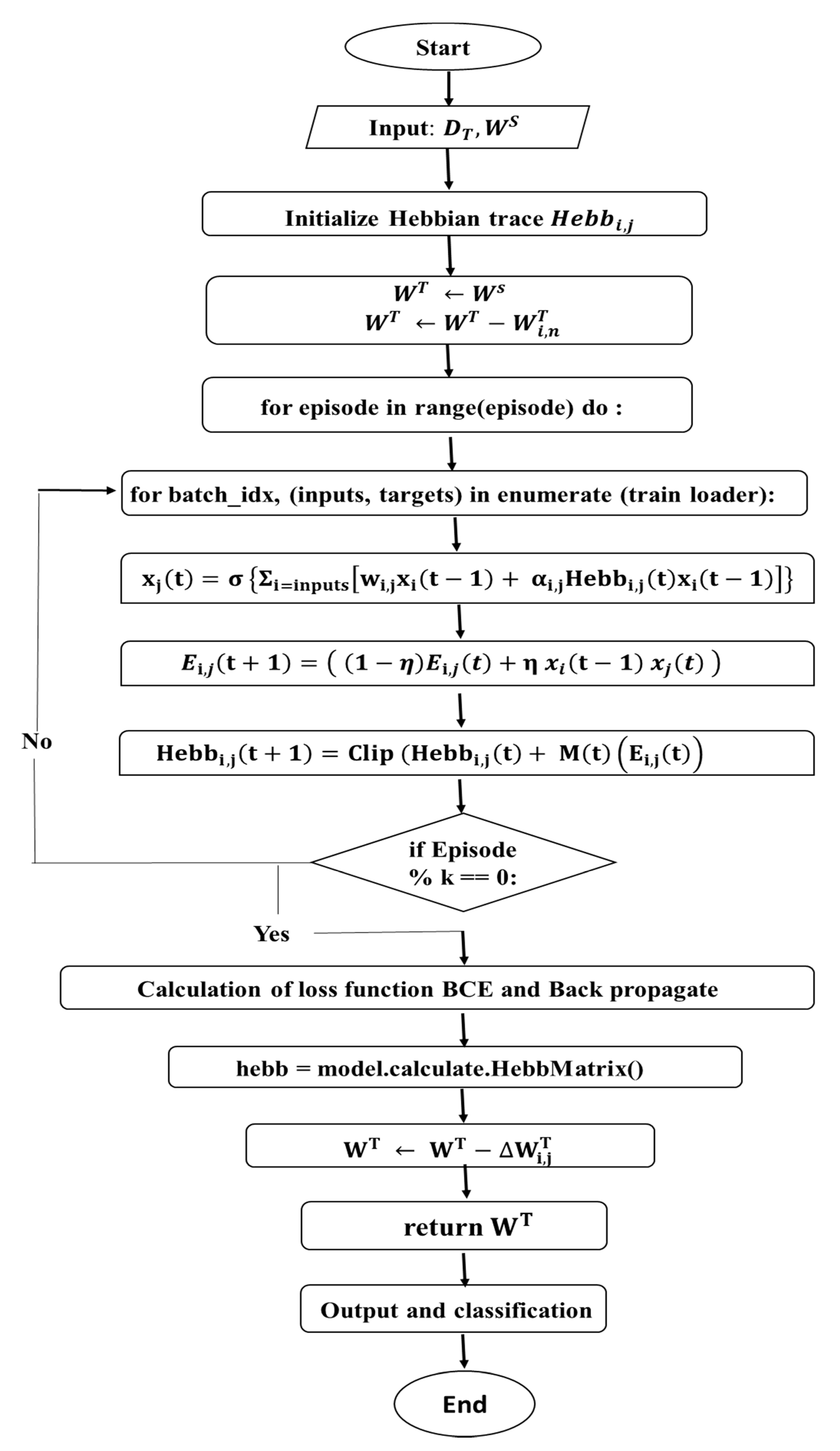
Figure 1 shows the flow chart describing the various steps and flow of control in the NDHTL algorithm. CNN architecture is kept the same for all the tasks to make experiments comparable for transfer learning. In the initial step, SGD training is applied to the source task. In the following step, the target task model is initialized with parameters learned from the previous step. In the last step, the Neuromodulated Dopamine Hebbian Transfer Learning algorithm has been applied to fine-tune the weights.

The Hebbian principles are used with a heterogeneous source and target datasets. Hebbian plasticity for connections can be modelled as a time-dependent quantity called Hebbian trace (${\mathrm{Hebb}}_{\mathrm{i},\mathrm{j}}$) [65]. The η parameter is a scalar value that automatically learns how quickly to consolidate new experiences into the plastic component. The value of the Hebb trace is calculated and stores as ${\mathrm{w}}_{\mathrm{i},\mathrm{j}}$and ${\mathrm{Hebb}}_{\mathrm{i},\mathrm{j}}$. We are using Equations (1) and (2). The symbol σ in Equation (2) defines non-linearity. It represents an activation function in the neural network. For example, tanh,

$${\mathrm{Hebb}}_{\mathrm{i},\mathrm{j}}\left(\mathrm{t}+1\right)={ \mathsf{\eta } \mathrm{x}}_{\mathrm{i}}\left(\mathrm{t}-1\right){\mathrm{x}}_{\mathrm{j}}\left(\mathrm{t}\right)+\left(1-\mathsf{\eta }\right){\mathrm{Hebb}}_{\mathrm{i},\mathrm{j}}\left(\mathrm{t}\right)$$

(1)

$${\mathrm{x}}_{\mathrm{j}}\left(\mathrm{t}\right)=\mathsf{\sigma } \left\{{{\displaystyle \sum }}_{i=inputs}\left[{\mathrm{w}}_{\mathrm{i},\mathrm{j}}{\mathrm{x}}_{\mathrm{i}}\left( \mathrm{t}-1\right)+{ \mathsf{\alpha }}_{\mathrm{i},\mathrm{j}}{\mathrm{Hebb}}_{\mathrm{i},\mathrm{j}}\left(\mathrm{t}\right){\mathrm{x}}_{\mathrm{i}}\left(\mathrm{t}-1\right)\right] \right\}$$

(2)

The ${\mathsf{\alpha }}_{\mathrm{i},\mathrm{j}}$ is a parameter for adjusting the magnitude of ${\mathrm{Hebb}}_{\mathrm{i},\mathrm{j}}$. The Hebb matrix accumulates mean hidden activations of the NDHTL layer for each target task. The pre-synaptic activations of neurons i in hidden compute the postsynaptic activations of neurons j.

Our approach implements transfer learning in the CNN network model with dopamine effects on plasticity. This technique is proposed to introduce neuromodulated plasticity within the transfer learning framework. Plasticity is modulated by a network controlled neuromodulatory signal, M(t), as shown in Equation (3).

M(t) is merely a single scalar output of the network, either used directly as a single value for all connections or passed through a vector of weights (one for each connection). Because η determines the rate of plastic change, placing it under network control allows the network to control how plastic connections should be at any given time. To balance the effects of both rises and dips in the baseline dopamine levels, M(t) can be positive or negative [88].

Hebbian plasticity uses eligibility trace to modify the synaptic weights indirectly; however, it creates a fast-decaying “potential” weight change, which is only applied to the actual weights if the synapse receives dopamine within a short time window. Each synapse is composed of a standard weight and a plastic (fast) weight that automatically increases or decreases due to continuous ongoing activity over time.

As a result, biological Hebbian traces practically implement a so-called eligibility trace [89], keeping the memory of what synapses contributed to recent activity, while the dopamine signal modulates the transformation of these eligibility traces into actual plastic changes.

$${\mathrm{Hebb}}_{\mathrm{i},\mathrm{j}}\left(\mathrm{t}+1\right)= \mathrm{Clip} ({\mathrm{Hebb}}_{\mathrm{i},\mathrm{j}}\left(\mathrm{t}\right)+ \mathrm{M}\left(\mathrm{t}\right)\left({\mathrm{E}}_{\mathrm{i},\mathrm{j}}\left(\mathrm{t}\right)\right))$$

(3)

$${\mathrm{E}}_{\mathrm{i},\mathrm{j}}\left(\mathrm{t}+1\right)=\left( \left(1-\mathsf{\eta }\right){\mathrm{E}}_{\mathrm{i},\mathrm{j}}\left(\mathrm{t}\right)+{\mathsf{\eta } \mathrm{x}}_{\mathrm{i}}\left(\mathrm{t}-1\right){ \mathrm{x}}_{\mathrm{j}}\left(\mathrm{t}\right) \right)$$

(4)

In Equations (3) and (4), the ${\mathrm{E}}_{\mathrm{i},\mathrm{j}}\left(\mathrm{t}\right)$ (the eligibility trace at connection i, j) is calculated as a simple exponential average of the Hebbian product of the pre- and post-synaptic activity, with trainable decay factor η ${\mathrm{Hebb}}_{\mathrm{i},\mathrm{j}}\left(\mathrm{t}\right)$. The dopamine signal M(t) is the tanh of the eligibility trace., the actual plastic component of the connection accumulates this trace but is gated by the current value of the dopamine signal M(t). M(t) is a symmetric value as calculated by a symmetric function.

The clip function restricts the value of the Hebbian matrix—the clip function, which is more biologically plausible, as it is not unbounded. In the algorithm below, on line number 7, the clamp function is used by setting the clip variable clipval to a minimum value such as 0.5. The clamp function from the PyTorch library uses clipval as the min and max value to clamp the float tensor within the min-max value. By doing so, the value of ${\mathrm{Hebb}}_{\mathrm{i},\mathrm{j}}\left(\mathrm{t}\right)$ is constrained within the clamp range and helps the Hebbian matrix values to grow disproportionately.

The one epoch of training is represented as one lifetime. In NDHTL algorithmic learning, we experimented with CNN architecture from [90] with SGD. The Hebb matrix is initialized to zero only at the start of learning the first task. This Hebbian update reflected in line 7 in the algorithm is repeated for each unique class in the target task. Quick learning, enabled by a highly plastic weight component, improves efficiency accuracy for a given task.

To prevent interference, the plastic component decays between the tasks and selective consolidation results in a stable component to preserve old memories, effectively enabling the model to learn to remember by modeling plasticity to form a learned neural memory. This allows it to scale efficiently with the increasing number of input tasks. The hidden activations are saved as compressed episodic memory in the Hebbian traces matrix to reflect individual episodic memory traces (similar to the work in the hippocampus in biological neural networks [91,92]).

Our model’s plastic component can be exploited and used for specific benefits by allowing gradient descent to optimize plastic connections. The model can alleviate the forgetting of consolidated classes by making connections less plastic to preserve the old information.

Furthermore, by making connections more plastic, the network can integrate and quickly learn new information. Our method encourages task-specific consolidation that alters the standard weights and plastic connection weights only where the change is required and keeps the irrelevant connection weight unchanged using the Hebbian matrix during the process.

The NDHTL Algorithm 1 can be defined as a biologically-motivated approach in computer vision, where simultaneous activation positively affects the increase in synaptic connection strength between the individual cells. The discriminative nature of learning for searching features in image classification fits well with the techniques, such as the Hebbian learning rule—neurons that fire together wire together.

In heterogeneous transfer learning, for such models, the connection weights of the learned model should adapt to the new target dataset with minimum effort. The discriminative learning rule, such as Hebbian learning, can improve learning performance by quickly adapting to discriminate between different classes defined by the target task. We apply the Hebbian principle as synaptic plasticity in heterogeneous transfer learning for the classification of heterogeneous.

A better algorithm will accommodate negative transfer, overfitting, and better synaptic weight consolidation processes. It solves challenges faced in heterogeneous scenarios of the transfer learning technique. It also uses biologically-proven Hebbian rules that form substantial connection weights and better connection paths from input to output of the neural network. Further, it has a better hybrid architecture. Similarly, the existing methods enhanced with plasticity will accommodate minor changes to the parameters of the CNN layers. That makes weights adaptation a quick and faster process.

This discriminating property of Hebbian learning employed with our proposed algorithm makes it a practical approach to techniques such as transfer learning. Relative minor weight fine-tuning using the pre and post spikes of a neural network-like structure enhances fine-tuning of the targeting of an unfamiliar dataset domain.

Algorithm 1: Neuromodulated Dopamine Hebbian Transfer Learning.

Input: $D_T, W^S$               // datasets Output: ${\mathrm{W}}^{\mathrm{T}}$                 //target connection weight 1: Initialize Hebbian trace $Heb{b}_{i,j}$         //Hebb plastic trace 2: $W^T \leftarrow W^S$                  //assign source weights to target 3: $W^T \leftarrow W^T-W_{i,n}^T$              //classification layer correction 4:   for episode in range(episode) do: for batch_idx, (inputs, targets) in enumerate (train loader): 5:      $x_j\left(t\right)=\sigma \left\{{\Sigma }_{i=inputs}\left[w_{i,j}{x}_i\left(t-1\right)+{\alpha }_{i,j}Heb{b}_{i,j}\left(t\right)x_i\left(t-1\right)\right]\right\}$ 6:      $E_{i,j}\left(t+1\right)=(\left(1-\eta \right)E_{i,j}\left(t\right)+\eta x_i\left(t-1\right) x_j\left(t\right)$) 7:     $Heb{b}_{i,j}\left(t+1\right)=Clip (Heb{b}_{i,j}\left(t\right)+M\left(t\right)\left(E_{i,j}\left(t\right)\right)$) 8:    if episode % k == 0: //k is a parameter 9:      Calculation of loss function BCE and Back propagate 10:     hebb = model.calculate.HebbMatrix() 11:     $W^T \leftarrow W^T-\Delta W_{i,j}^T$ 12:   return $W^T$

3.3. CNN Hybrid Architecture

The hybrid NDHTL architecture is from [90] with modifications. Furthermore, $Heb{b}_{i,j}$ plastic connections, and the NDHTL plastic layer, has been added at the end of the CNN. The NDHTL plastic layer following the five convolutional layers has ${\mathrm{Hebb}}_{\mathrm{i},\mathrm{j}}$. The Hebbian trace defines every value of connection weight plasticity. The filter configuration of different layers is 64, 192, 384, 256, and 256, as shown in Figure 2.

4. Experiments

4.1. Datasets

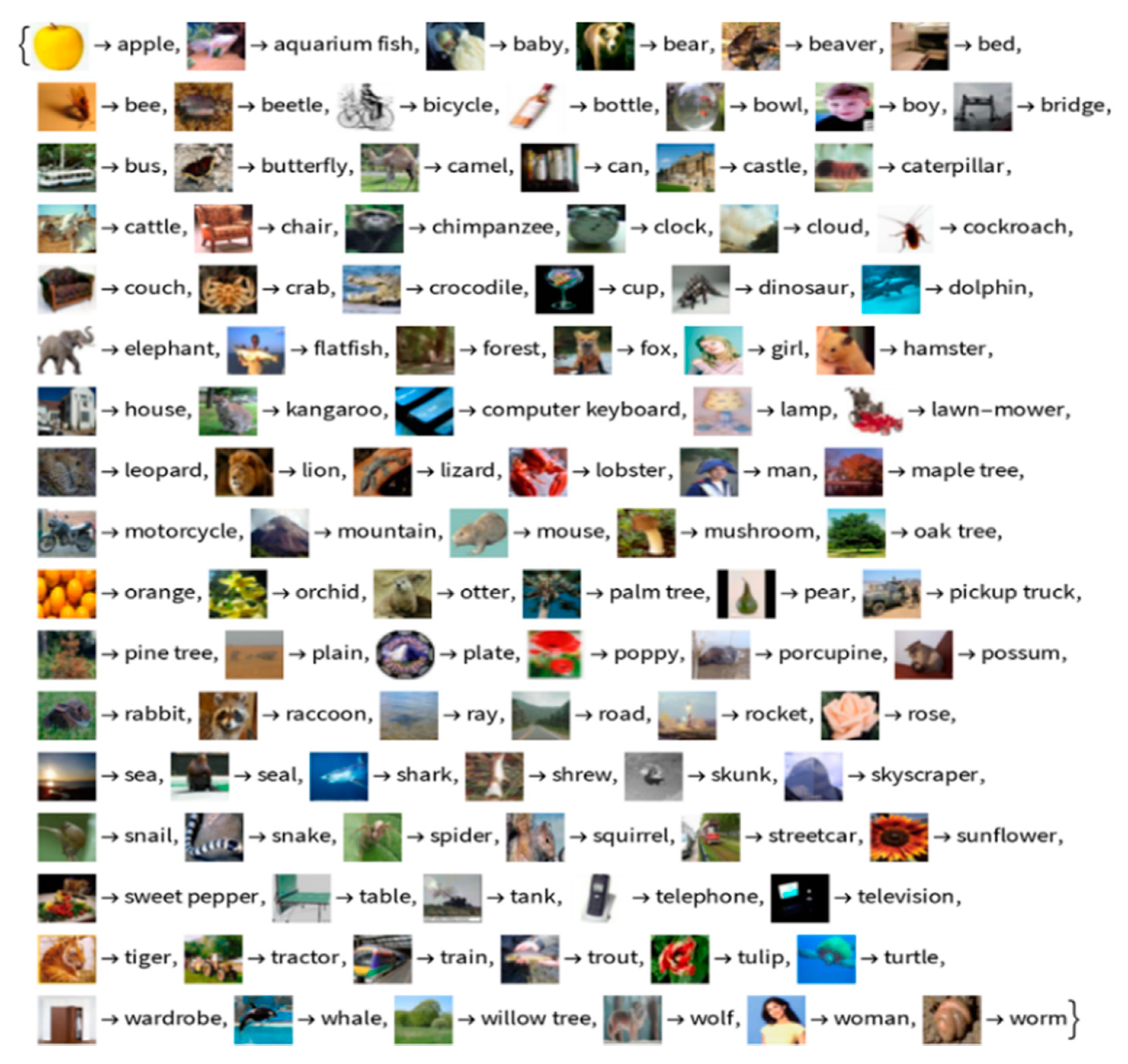
In experiments, we use the source dataset CIFAR-10 and target domain CIFAR-100. Figure 3 and Figure 4 show example images.

We use all class categories of the CIFAR-10 dataset to calculate the source model weights ${\mathrm{W}}^{\mathrm{S}}$. The CIFAR-10 source dataset includes truck, ship, horse, frog, dog, deer, cat, bird, automobile, and airplane. We made ten different subsets of CIFAR-100 categories for the target domain by grouping similar superclasses together, as shown in

Table 2. The CIFAR-100 target data categories.

Dataset	Classes (Union of Similar 2 Super Classes)
${\mathrm{T}}_1$	aquatic mammals + fish: trout, shark, ray, flatfish, aquarium fish, whale, seal, otter, dolphin, beaver
${\mathrm{T}}_2$	flowers + fruit and vegetables: sweet peppers, pears, oranges, mushrooms, apples, tulips, sunflowers, roses, poppies, orchids
${\mathrm{T}}_3$	food containers + household electrical devices: television, telephone, lamp, computer keyboard, clock, plates, cups, cans, bowls, bottles
${\mathrm{T}}_4$	household furniture + large man-made outdoor things: skyscraper, road, house, castle, bridge, wardrobe, table, couch, chair, bed
${\mathrm{T}}_5$	insects + non-insect invertebrates: worm, spider, lobster, crab, cockroach, caterpillar, butterfly, beetle, snail, bee
${\mathrm{T}}_6$	medium-sized mammals+small mammals: kangaroo, elephant, chimpanzee, cattle, camel, wolf, tiger, lion, leopard, bear
${\mathrm{T}}_7$	medium-sized mammals+small mammals: squirrel, rabbit, shrew, mouse, hamster, skunk, raccoon, possum, porcupine, fox,
${\mathrm{T}}_8$	people + reptiles: turtle, snake, lizard, dinosaur, crocodile, woman, man, girl, boy, baby
${\mathrm{T}}_9$	trees + large natural outdoor scenes: sea, plain, mountain, forest, cloud, willow, palm, oak, pine, maple,
${\mathrm{T}}_{10}$	vehicles 1 + vehicles2: tractor, tank, rocket, streetcar, lawn-mower, train, pickup truck, motorcycle, bicycle, bus

.

4.2. Experimental Setup

Training begins with the source CIFAR-10 classification task with learning rates 0.0001 and 0.1. Under our experimental setup, we use cross-entropy loss. This works in phases, where a lifetime is mapped to one epoch or one cycle of the fine-tuning process [81].

The meta-parameter—$\mathsf{\eta }$, defines the plasticity rate of the algorithm. The n is the number of episodes in one lifetime of the algorithm. The NDHTL technique uses an input image batch size of 1 for every algorithm step. The same is used for the iteration of the forward propagation for the NDHTL hybrid neural network architecture.

Followed by value consolidation with the Hebb trace matrix, the last step for every episode is to calculate the loss and perform connection weight consolidation and synaptic consolidation following the backpropagation of the network that updates ${\mathrm{w}}_{\mathrm{i},\mathrm{j}}$ and ${\mathsf{\alpha }}_{\mathrm{i},\mathrm{j}}$. Then, the re-initialization of the Hebbian matrix is performed at each episode’s end.

We also need to compute eta-$\mathsf{\eta }$—(the plasticity rate), determined by neuromodulation. The network independently decides the “eta” of the connection weights and plasticity percentage of the neural connections such as the dopamine system. Inside the brain, dopamine controls dopaminergic cell systems and pathways, neuromodulation, and functions in reinforcement and reward. In NDHTL, the neural network layers output controls eta—the plastic nature of the connection weights, which controls the transfer learning efficacy and accuracy on the model altogether.

In NDHTL, unlike traditional backpropagation, which is a symmetric system for gradient backpropagation. The NDHTL gradient is backpropagated asymmetrically at the end of the episodes following the classification loss function calculation mentioned in the paragraph below.

To calculate the gradient, the loss is calculated using Equation (5), and the gradient is backpropagated. For keeping the configuration comparable, i.e., the validation loss function used in NDHTL is kept the same as the one used in standard transfer learning setup, cross-entropy.

$$\mathrm{BCE}=-\frac{1}{\mathrm{N}}{{\displaystyle \sum }}_{\mathrm{i}=0}^{\mathrm{N}}{\mathrm{y}}_{\mathrm{i}}.\log \left({\mathrm{y}}_{\mathrm{i}}^{^}\right)+\left(1-{\mathrm{y}}_{\mathrm{i}}\right).\log \left(1-{\mathrm{y}}_{\mathrm{i}}^{^}\right)$$

(5)

We collect the percentage of average validation loss, validation accuracy top-1, and validation accuracy top-5 accuracy values for each lifetime during training, followed by validation dataset testing. In standard transfer learning, the SGD is implemented in the STL algorithm for all the iterations in the dataset. Contrary to the STL and NDHTL transfer learning, the algorithm only back propagates at the end of each episode controlled by hyper parameter K.

In the NDHTL algorithm, the hyper parameter K controls when the algorithm performs backpropagation. In STL, N is the number of feedforward steps, and N is the number of backpropagation steps. In NDHTL, N is the total number of feedforward steps; however, N/ K is the number of backpropagation steps. A similar number of cost function calculations and reductions are performed. So, we can say NDHTL is theoretically computing quicker than STL. However, we also have a Hebb matrix in NDHTL computed for the same number of feedforward steps. We may say that the time saved by performing fewer backpropagation steps by the algorithm is helping in the time consumed in Hebbian matrix plastic weight calculations.

4.3. Experimental Results

In the NDHTL learning method, we use the feature–extraction layer and reweigh the output layer, followed by fine-tuning using an NDHTL algorithm to determine if the parameter distribution difference between the source and task dataset is reduced. Our algorithm is generic and can be extended to any neural network architecture with feature extraction and plastic NDHTL classification layer integration. The experimental results showed that the NDHTL achieves better accuracy than the STL method. The average top-1 accuracy improvements are 1.3%. Based on experimental results, we may say that the NDHTL algorithm achieves much better performance when the heterogeneous source and target domain are used.

Table 3. Top-5 and Top-1 result table for validation accuracy of NDHTL & STL.

Metric	Target	STL	NDHTL	Improvement
Top-1 accuracy	${\mathrm{T}}_1$	59.6%	60.7%	+1.10%
	${\mathrm{T}}_2$	69.9%	73.1%	+3.20%
	${\mathrm{T}}_3$	65.0%	65.9%	+0.90%
	${\mathrm{T}}_4$	75.0%	75.6%	+0.60%
	${\mathrm{T}}_5$	67.9%	68.8%	+0.90%
	${\mathrm{T}}_6$	63.0%	63.9%	+0.90%
	${\mathrm{T}}_7$	57.0%	57.6%	+0.60%
	${\mathrm{T}}_8$	51.6%	55.2%	+3.60%
	${\mathrm{T}}_9$	73.7%	74.0%	+0.30%
	${\mathrm{T}}_{10}$	74.4%	75.3%	+0.90%
Average		65.71%	67.01%	+1.3%
Top-5 accuracy	${\mathrm{T}}_1$	94.7%	96.5%	+1.80%
	${\mathrm{T}}_2$	97.3%	97.9%	+0.60%
	${\mathrm{T}}_3$	94.9%	96.0%	+1.10%
	${\mathrm{T}}_4$	97.8%	98.4%	+0.60%
	${\mathrm{T}}_5$	95.0%	95.7%	+0.70%
	${\mathrm{T}}_6$	94.0%	94.4%	+0.40%
	${\mathrm{T}}_7$	91.0%	91.9%	+0.90%
	${\mathrm{T}}_8$	95.5%	96.3%	+0.30%
	${\mathrm{T}}_9$	99.0%	99.4%	+0.40%
	${\mathrm{T}}_{10}$	97.9%	98.2%	+0.30%
Average		95.71	96.37	+0.71%

displays the standard transfer learning (STL) and NDHTL in top-1 and top-5 validation accuracy for the setup described in Section 4.2.

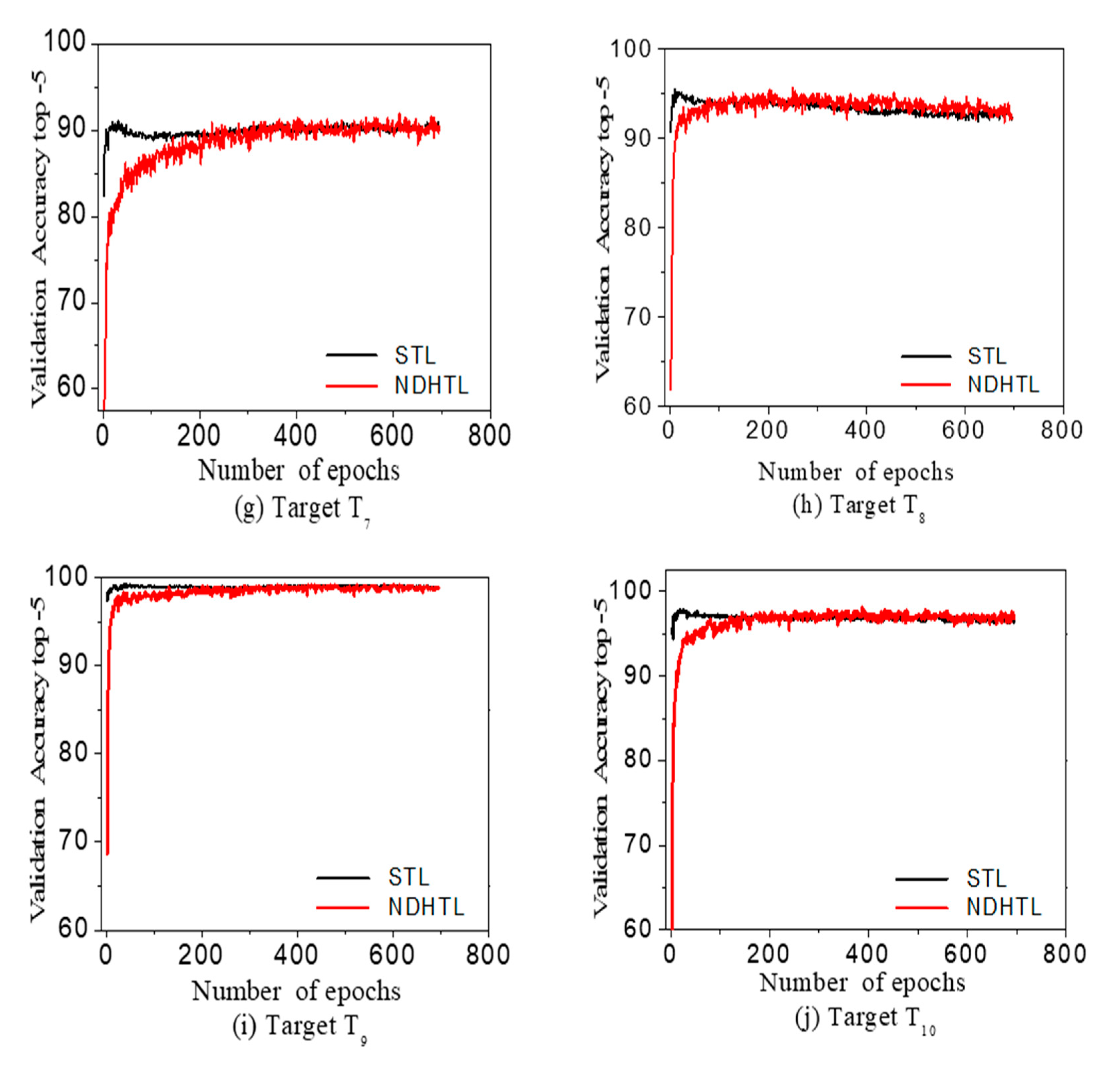
The STL and NDHTL study data plots are shown for ten different datasets in terms of the top-5 accuracy in Figure 5. The data curves for STL and NDHTL for the CIFAR100 target dataset (${\mathrm{T}}_{1–10}$), shows a significant improvement in the top-5 accuracy for the NDHTL algorithm. The experimental results are shown in Table 3 and Figure 5.

The source is kept the same as the CIFAR-10, and the target datasets are different from the dataset ${\mathrm{t}}_1$ to dataset ${\mathrm{t}}_{10}$. The target task performance is different with different target datasets, as in Figure 5 and Table 3 for top-1 and top-5. To understand the overall effect, the algorithm’s average performance over all the datasets is calculated as shown in Table 3. Average values of performance over the ten datasets shows significant improvement as compared to the standard method.

In particular, a significant improvement of +3.60% with NDHTL implies that the NDHTL is more effective for transfer learning between heterogeneous source and target. The average improvement in the top-1 accuracy with NDHTL is +1.30%, and improvement with the top-5 accuracy is +0.71%.

Keeping the goal of transfer learning in mind, wherein the scenario where what has been learned in one setting is exploited to improve generalization in another setting. Furthermore, speaking from practical experience, the source model training must be performed by randomly initializing the network. While partially training the network, the weight values are generic and can quickly adapt or fine-tune to any random target task datasets.

Overtraining the source model may result in poor transfer learning accuracy on the target task dataset. We are keeping the image classification task in the context of the explanation.

Based on the experimental results, we may conclude that heterogeneous datasets serve as the best source task for Hebbian transfer learning classification. Indeed, extensive data were collected by experimenting with more than ten different datasets and a similar number of experiments. We may conclude that the Hebbian transfer learning algorithm is much better with validation accuracy improvement than standard transfer learning algorithms.

5. Discussion on Applications

The introduction of biologically inspired neuromodulated dopamine effects on plastic transfer learning has been studied in detail by performing multiple experiments. This paper presents a novel NDHTL algorithm that is extendable to multiple domains from an application point of view. NDHTL, combined with traditional CNN approaches, is an efficient approach. The algorithm can be easily extended to related deep learning neural network domains.

We do not claim that such an asymmetric backpropagation algorithm is implemented in the brain. However, evolutionary learning contributes to learning in an animal’s brain. The brain’s resulting self-modifying abilities play an important role in learning and adaptation and constitute a significant basis for biological memorization and learning sustainability. In the literature survey, dopamine is shown to repeatedly manage the plasticity induced by a recent past event within a short time window of about 1 s [93,94,95,96,97]. Such procedures have been modeled in computational neuroscience studies. The paper also introduces the neuromodulation scheme that takes inspiration from the short-term retroactive effects of neuromodulatory dopamine on Hebbian plasticity in animal brains. The backpropagation of the plastic layer for Hebbian learning has been previously studied as well. However, this new study of plasticity and dopamine neuromodulation plays an essential role in learning and adaptation.

Aiming at the image classification model of learning on big datasets, some researchers propose a technique to solve the problem of scene–object recognition in T.V. programs, such as movies, T.V. plays, variety shows, and short videos, by transferring a pre-trained depth image classification model to a specific task. Many personalized advertisement recommendation studies suffer from the problem that only certain tagged items can be recommended in video playback. In such attempts to adopt transfer knowledge to solve data volume problems, providing users with various options is applicable. We often encounter situations where an insufficient amount of high-quality data in a target domain may have plenty of auxiliary data in related domains. Transfer learning aims to exploit additional data to improve the learning performance in the target domain. Innovative transfer learning applications include learning in heterogeneous cross-media domains, online recommendation, social media, and social network mining.

Transfer learning has been applied to alleviate the data scarcity problem in many urban computing applications. For example, chain store site recommendation leverages the knowledge from semantically relevant domains to the target city. A possible solution is a flexible multi-modal transfer learning to the target city to alleviate the data scarcity problem.

Another widely encountered task in the bioinformatics domain is gene expression analysis, e.g., predicting associations between genes and phenotypes. There is usually very little data of the known associations. In such an application, one of the main challenges is the data sparsity problem. As a potential solution, transfer learning can be used to leverage additional information and knowledge. For example, they use a transfer learning approach to analyze and predict the gene–phenotype associations based on the Label Propagation Algorithm (LPA). In addition to Wi-Fi localization tasks, transfer learning has also been employed in wireless network applications. Transfer learning applications, such as those that can be applied to the recognition of tasks for hand gesture recognition, face recognition, activity recognition, and speech emotion recognition can also be applied to learn driver pose recognition. Similarly, NDHTL can be utilized for anomalous activity detection, and traffic sign recognition.

In addition to imaging analysis, transfer learning has other applications in the medical area. Deep learning has been applied to identify, detect, and diagnose breast cancer risk analysis. Transfer learning for pediatric pneumonia diagnosis and lung pattern analysis is beneficial. Applying transfer learning in biomedical image analysis is a promising domain and supports a general-purpose cause.

NDHTL transfer learning may be applied in NLP natural language processing. NDHTL transfer-learning expertise may also be incorporated into sentiment analysis, fraud detection, social networks, and hyperspectral image analysis. With a large amount of data related to our cities, for example, computing in traffic monitoring directions, health care, social security, the world needs algorithms such as NDHTL for better problem-solving approaches.

6. Conclusions

In transfer learning with deep learning, the training data is usually from a similar domain or shares the feature space, and the data distribution is symmetrical and does not change much over many iterations. The discriminative learning rule, such as Hebbian learning, can improve learning performance by quickly adapting to discriminate between different classes defined by target task. We apply the Hebbian principle as synaptic plasticity in heterogeneous transfer learning to classify images using a heterogeneous source–target dataset and compare results with the standard transfer learning case. Hebbian learning is a form of discriminative learning to search for the specific feature for object recognition or image classification activity-dependent synaptic plasticity where correlated activation of pre- and post-synaptic neurons leads to strengthening the connection between the two neurons. Hebbian plasticity is a form of synaptic plasticity induced by and further amplifies correlations in neuronal activity.

However, in real-world situations, the data is of variable distribution with ever-changing nature. A dynamic technique that uses hyperparameters and adjusts to target tasks by manipulating during the time may significantly improve the learning efficiency of an algorithm. In this paper, implementing such a solution for the heterogeneous transfer learning domain, a neuromodulated dopamine transfer learning algorithm based on the Hebbian learning principle is presented.

We investigated the use of neuromodulated dopamine-controlled synaptic plasticity implementing the Hebbian theory using plasticity and asymmetric backpropagation, and applied it to heterogeneous transfer learning.

The NDHTL algorithm is a generic cross-domain CNN training algorithm. Using plastic NDHTL layer integration, the fine-tuning of the CNN weights is easily accomplished. In implementing NDHTL, minimum alteration of the weights is required to fine-tune the target dataset by synaptic weight consolidation. In the NDHTL transfer learning algorithm, a hybrid architecture is initialized with a pretrained model from the source task, and the last layer is re-weighted. Following which the model is fine-tuned to a target task.

By using the NDHTL algorithm, the connection–weight–parameter distribution difference between source and target task is quickly reduced. It may be applied to scenarios with negative transfer where the goal for transfer learning is to enhance the performance of a target task using an auxiliary/source domain. The issue becomes that sometimes transferring knowledge from a source domain may have a negative impact on the target model. This is also known as a negative transfer. This occurs primarily when the source domain has very little in common with the target. The NDHTL algorithm is a possible solution to such issues in transfer learning.

The algorithm is easily extendible to similar problems, given that the corresponding solution aims to implement neural network architecture with a weight–extraction and cost–function reduction design.

Experiments were conducted to compare the efficiency of the proposed algorithm with standard transfer learning. The experiment used CIFAR-10 as the source domain and CIFAR-100 as the target domain.

A CIFAR-10 source and CIFAR-100 target dataset were studied implementing NDHTL, and we concluded that asymmetric NHDTL achieves better accuracy than the symmetric STL method based on the data generated as the output.

The recorded average top-1 accuracy improvements are 1.3%. Based on experimental results, we may conclude that the NDHTL algorithm performs much better with cross-domain image classification and heterogeneous source and target transfer learning tasks.

The experimental results showed that the NDHTL achieves better accuracy than the STL method, precisely when the heterogeneous source and target domain are used. Experiments with fully plastic and neuromodulated plastic CNN architectures for quick training and better performance are possible in the future. Researchers may investigate the application of NDHTL techniques other than for image datasets.

References

- Albawi, S.; Mohammed, T.A.; Al-Zawi, S. Understanding of a convolutional neural network. In Proceedings of the 2017 International Conference on Engineering and Technology (I.C.E.T.), Antalya, Turkey, 21–23 August 2017; pp. 1–6. [Google Scholar]
- Rajpurkar, P.; Irvin, J.; Ball, R.L.; Zhu, K.; Yang, B.; Mehta, H.; Duan, T.; Ding, D.; Bagul, A.; Langlotz, C.P.; et al. Deep learning for chest radiograph diagnosis: A retrospective comparison of the CheXNeXt Algorithm to practicing radiologists. PLoS Med. 2018, 15, e1002686. [Google Scholar] [CrossRef] [PubMed]
- Bottou, L. Stochastic gradient tricks. In Neural Networks, Tricks of the Trade, Reloaded, Lecture Notes in Computer Science (LNCS 7700); Montavon, G., Orr, G.B., Muller, K.-R., Eds.; Springer: Berlin/Heidelberg, Germany, 2012; pp. 430–445. [Google Scholar]
- Lagani, G. Hebbian Learning Algorithms for Training Convolutional Neural Networks–Project Code. 2019. Available online: https://github.com/GabrieleLagani/HebbianLearningThesis (accessed on 13 June 2021).
- Izhikevich, E.M. Solving the distal reward problems through linkage of S.T.D.P. and dopamine signaling. Cereb. Cortex 2007, 17, 2443–2452. [Google Scholar] [CrossRef] [PubMed] [Green Version]
- McCloskey, M.; Cohen, N.J. Catastrophic Interference in Connectionists Networks: The Sequential Learning Problem. Psychol. Learn. Motiv. 1989, 24, 109–165. [Google Scholar]
- French, R. Catastrophic Forgetting in Connectionist Networks. Trends Cogn. Sci. 1999, 3, 128–135. [Google Scholar] [CrossRef]
- Ring, M.B. Continual Learning in Reinforcement Environments. Ph.D. Thesis, University of Texas at Austin, Austin, TX, USA, 1994. [Google Scholar]
- Thrun, S.; Mitchell, T. Lifelong robot learning. Robot. Auton. Syst. 1995, 15, 25–46. [Google Scholar] [CrossRef]
- Carpenter, G.A.; Grossberg, S. A massively parallel architectures for a self-organising neural pattern recognition machine. Comput. Vis. Graph. Image Process. 1987, 37, 54–115. [Google Scholar] [CrossRef]
- Abraham, W.C.; Robins, A. Memory Retention–The Synaptic Stability Versus Plasticity Dilemma. Trends Neurosci. 2005, 28, 73–78. [Google Scholar] [CrossRef]
- Gerstner, W.; Kistler, W.M. Spiking Neuron Models: Single Neurons, Populations, Plasticity; Cambridge University Press: Cambridge, UK, 2002. [Google Scholar]
- Haykin, S. Neural Networks and Learning Machines/Simon Haykin, 3rd ed.; Prentice Hall: New York, NY, USA, 2009. [Google Scholar]
- Liu, N.; Wan, L.; Zhang, Y.; Zhou, T.; Huo, H.; Fang, T. Exploiting convolutional neural networks with deeply local description for remote sensing image classification. IEEE Access 2018, 6, 11215–11228. [Google Scholar] [CrossRef]
- Milletari, F.; Navab, N.; Ahmadi, S.-A. V-Net: A Fully Convolutional Neural Networks for Volumetric Medical Image Segmentation. In Proceedings of the 2016 Fourth International Conference on 3D Vision (3DV), Stanford, CA, USA, 25–28 October 2016. [Google Scholar]
- Robbins, H.; Monro, S. A stochastic approximation method. Ann. Math. Stat. 1951, 22, 400–407. [Google Scholar] [CrossRef]
- Wang, S.; Ma, S.; Yuan, Y.-X. Penalty methods with a stochastic approximation for stochastic nonlinear programming. Math. Comp. 2017, 86, 1793–1820. [Google Scholar] [CrossRef]
- Nemirovski, A.; Juditsky, A.; Lan, G.; Shapiro, A. Robust stochastic approximation approach to stochastic programming. SIAM J. Optim. 2019, 19, 1574–1609. [Google Scholar] [CrossRef] [Green Version]
- Krizhevsky, A.; Sutskever, I.; Hinton, G.E. Imagenets classification with deep convolutional neural networks. Adv. Neural Inform. Process. Syst. 2012, 25, 1097–1105. [Google Scholar] [CrossRef]
- Simonyan, K.; Zisserman, A. Very deep convolutional networks for large-scale images recognition. In Proceedings of the 3rd International Conferences on Learning Representations 2015, San Diego, CA, USA, 7–9 May 2015. [Google Scholar]
- Tan, C.; Sun, F.; Kong, T.; Zhang, W.; Yang, C.; Liu, C. A survey on deep transfer learning. In Proceedings of the International Conferences on artificial Neural Networks 2018, Rhodes, Greece, 4–7 October 2018. [Google Scholar]
- Wang, M.; Deng, W. Deep visual domain adaptation: A survey. Neurocomputing 2018, 312, 135–153. [Google Scholar] [CrossRef] [Green Version]
- Saito, K.; Watanabe, K.; Ushiku, Y.; Harada, T. Maximum classifier discrepancy for unsupervised domain adaptation. In Proceedings of the IEEE /CVF Conference on Computer Vision and Pattern Recognition 2018, Salt Lake City, UT, USA, 19–21 June 2018. [Google Scholar]
- Greenspan, H.; Van Ginneken, B.V.; Summers, R.M. Guest editorial deep learning in medical imaging: Overview and future promises of an exciting new technique. IEEE Trans. Med. Imaging 2016, 35, 1153–1159. [Google Scholar] [CrossRef]
- Ching, T.; Himmelstein, D.S.; Beaulieu-Jones, B.K.; Kalinin, A.A.; Do, B.T.; Way, G.P.; Ferrero, E.; Agapow, P.M.; Zietz, M.; Hoffman, M.M.; et al. Opportunities and obstacles for deep learning in biology and medicine. J. R. Soc. Interface 2018, 15, 20170387. [Google Scholar] [CrossRef] [PubMed] [Green Version]
- Dan, Y.; Poo, M.-M. Spike timing-dependent plasticity of neural circuits. Neuron 2004, 44, 23–30. [Google Scholar] [CrossRef] [PubMed] [Green Version]
- Amato, G.; Carrara, F.; Falchi, F.; Gennaro, C.; Lagan, G. Hebbian learning meets deep convolutional neural networks. In Proceedings of the I.C.I.A.P. 2019: Image Analysis and Processing 2019, Trento, Italy, 9–13 September 2019. [Google Scholar]
- Hubel, D.H.; Wiesel, T.N. Receptive fields, binocular interaction, and functional architecture in the cat’s visual cortex. J. Physiol. 1962, 160, 106–154. [Google Scholar] [CrossRef]
- Miconi, T. Backpropagation of Hebbian plasticity for continual learning. In Proceedings of the Conference on Neural Information Processing Systems (NIPS) Workshop on Continual Learning 2016, Barcelona, Spain, 5–10 December 2016. [Google Scholar]
- Bang, S.H.; Ak, R.; Narayanan, A.; Lee, Y.T.; Cho, H.B. A survey on knowledge transfer for manufacturing data analytics. Comput. Ind. 2019, 104, 116–130. [Google Scholar] [CrossRef]
- Zhuang, F.; Qi, Z.; Duan, K.; Xi, D.; Zhu, Y.; Zhu, H.; Xiong, H.; He, Q. A Comprehensive Survey on Transfer Learning. arXiv 2019, arXiv:1911.02685. [Google Scholar] [CrossRef]
- Weiss, K.; Khoshgoftaar, T.M.; Wang, D.D. A survey of transfer learning. J. Big Data 2016, 3, 1345–1359. [Google Scholar] [CrossRef] [Green Version]
- Agarwal, N.; Sondhi, A.; Chopra, K.; Singh, G. Transfer learning: Survey and classification. In Part of the Advance in Intelligent Systems and Computing; Springer: Berlin/Heidelberg, Germany, 2021; Volume 1168. [Google Scholar]
- Krizhevsky, A.; Sulskever, I.; Hinton, G.E. ImageNet classification with deep convolutional neural networks. ACM Digit. Libr. 2017, 60, 84–90. [Google Scholar] [CrossRef]
- Bengio, Y.; Bengio, S.; Cloutier, J. Learning a synaptic learning rule. In Proceedings of the International Joint Conferences on Neurel Networks, Seattle, WA, USA, 8–12 July 1991. [Google Scholar]
- Schmidhuber, J. Learning to control fast-weight memories: An alternative to dynamic recurrent networks. Neural Comput. 1992, 4, 131–139. [Google Scholar] [CrossRef]
- Ojala, T.; Pietikainen, M.; Maenpaa, T. Multiresolutions gray-scale and rotations invariant texture classification with local binary patterns. IEEE Trans. Pattern Anal. Mach. Intell. 2002, 24, 971–987. [Google Scholar] [CrossRef]
- Liang, G.; Zheng, L. A transfer learning method with the deep residual network for pediatric pneumonia diagnosis. Comput. Methods Programs Biomed. 2020, 187, 104964–104972. [Google Scholar] [CrossRef]
- Raghu, M.; Zhang, C.; Kleinberg, J.; Bengio, S. Transfusion: Understanding transfer learning for medical imaging. In Proceedings of the Conference on Neurel Information Processing Systems (NIPS), Vancouver, BC, Canada, 8–14 December 2019. [Google Scholar]
- Sevakula, R.K.; Singh, V.; Verma, N.K.; Kumar, C.; Cui, Y. Transfer learning for molecular cancer classification using deep neural networks. IEEE/ACM Trans. Comput. Biol. Bioinform. 2019, 16, 2089–2100. [Google Scholar] [CrossRef] [PubMed]
- Huynh, B.Q.; Li, H.; Giger, M.L. Digital mammographic tumor classification using transfer learning from deep convolutional neural networks. J. Med. Imaging 2016, 3, 034501. [Google Scholar] [CrossRef]
- Akçay, S.; Kundegorski, M.E.; Devereux, M.; Breckon, T.P. Transfer learning using convolutional neural networks for object classification within X-ray baggage security imagery. In Proceedings of the IEEE International Conferences on Image Processing 2016, Phoenix, AZ, USA, 25–28 September 2016. [Google Scholar]
- Shao, L.; Zhu, F.; Li, X. Transfer Learning for Visual Categorization: A Survey. IEEE Trans. Neural Netw. Learn. Syst. 2015, 26, 1019–1034. [Google Scholar] [CrossRef] [PubMed]
- Hebb, D.O. The Organization of Behavior; A Neuropsychological Theory; Wiley: Oxford, UK, 1949. [Google Scholar]
- Paulsen, O.; Sejnowski, T.J. Natural patterns of activity and long-term synaptic plasticity. Curr. Opin. Neurobiol. 2000, 10, 172–179. [Google Scholar] [CrossRef] [Green Version]
- Song, S.; Miller, K.D.; Abbott, L.F. Competitive Hebbian learning through spike-timing-dependent synaptic plasticity. Nat. Neurosci. 2000, 3, 919–926. [Google Scholar] [CrossRef]
- Oja, E. Oja learning rule. Scholarpedia 2008, 3, 3612. [Google Scholar] [CrossRef]
- Zenke, F.; Gerstner, W.; Ganguli, S. The temporal paradox of Hebbian learnings and homeostatic plasticity. Curr. Opin. Neurobiol. 2017, 43, 166–176. [Google Scholar] [CrossRef] [Green Version]
- Hebb, D.O. Physiological learning theory. J. Abnorm. Child Psychol. 1976, 4, 309–314. [Google Scholar] [CrossRef]
- Rae, J.W.; Dyer, C.; Dayan, P.; Lillicrap, T.P. Fast parametric learning with activation memorization. In Proceedings of the 35th International Conference on Machine Learning, Stockholm, Sweden, 10–15 July 2018. [Google Scholar]
- Thangarasa, V.; Miconi, T.; Taylor, G.W. Enabling Continual Learning with Differentiable Hebbian Plasticity. In Proceedings of the 2020 International Joint Conference on Neural Networks (IJCNN), Glasgow, UK, 19–24 July 2020; pp. 1–8. [Google Scholar] [CrossRef]
- Kirkpatrick, J.; Pascanu, R.; Rabinowitz, N.C.; Veness, J.; Desjardins, G.; Rusu, A.A.; Milan, K.; Quan, J.; Ramalho, T.; Barwinska, A.G.; et al. Overcomng catastrophic forgetting in neurel networks. Proc. Natl. Acad. Sci. USA 2017, 114, 3521–3526. [Google Scholar] [CrossRef] [Green Version]
- Zenke, F.; Poole, B.; Ganguli, S. Continual learning through synaptic intelligence. In Proceedings of the 34th International Conference on Machine Learning (I.C.M.L.), Sydney, Australia, 6–11 August 2017. [Google Scholar]
- Kandel, E.R. The molecular biology of memory storage: A dialogue between genes and synapses. Science 2001, 294, 1030–1038. [Google Scholar] [CrossRef] [Green Version]
- Parisi, G.I.; Kemker, R.; Part, J.L.; Kanan, C.; Wermter, S. Continual lifelong learning with neural network: A review. Neural Netw. 2019, 113, 54–71. [Google Scholar] [CrossRef] [PubMed]
- Thorne, J.; Vlachos, A. Elastic weight consolidation for better bias innoculation. In Proceedings of the 16th conferences of the European Chapter of the Association for Computational Linguistic (EACL), Online, 19–23 April 2021. [Google Scholar]
- Zenke, F.; Poole, B.; Ganguli, S. Improved Multitask Learning through Synaptic Intelligence. arXiv 2017, arXiv:1703.04200. [Google Scholar]
- Aljundi, R.; Babiloni, F.; Elhoseiny, M.; Rohrbach, M.; Tuytelaars, T. Memory aware synapse: Learning what (not) to forget. In Proceedings of the European Conference on Computer Vision (E.C.C.V.), Munich, Germany, 8–14 September 2018. [Google Scholar]
- Hinton, G.E.; Plaut, D.C. Using fast weights to deblur old memories. In Proceedings of the 9th Annual Conferences of the Cognitive Science Society, Seattle, WA, USA, 16–18 July 1987. [Google Scholar]
- Medwin, A.R.G. Doubly modifiable synapse: A model of short and long term auto-associative memories. Proc. R. Soc. B Biol. Sci. 1989, 238, 137–154. [Google Scholar]
- Kermiche, N. Contrastive Hebbian Feedforward Learning for Neural Networks. IEEE Trans. Neural Netw. Learn. Syst. 2020, 31, 2118–2128. [Google Scholar] [CrossRef] [PubMed]
- Munkhdalai, T.; Trischler, A. Metalearning with Hebbian Fast Weights. arXiv 2018, arXiv:1807.05076. [Google Scholar]
- Miconi, T.; Thangarasa, V. Learning to Learn with Backpropagation of Hebbian Plasticity. arXiv 2016, arXiv:1609.02228. [Google Scholar]
- Miconi, T.; Stanley, K.O.; Clune, J. Differentiable plasticty: Training plastic neural networks with backpropagation. In Proceedings of the 35th International Conferences on Machine Learning (I.C.M.L.), Stockholm, Sweden, 10–15 July 2018. [Google Scholar]
- Miconi, T.; Rawal, A.; Clune, J.; Stanley, K.O. Backpropamine: Training Self-modifying Neural Networks with Differentiable Neuromodulated Plasticity. In Proceedings of the 7th International Conference on Learning Representations, ICLR 2019, New Orleans, LA, USA, 6–9 May 2019. [Google Scholar]
- Fukushima, K. Neocognitron: A hierarchical neural network capable of visual pattern recognition. Neural Netw. 1988, 1, 119–130. [Google Scholar] [CrossRef]
- Krishna, S.T.; Kalluri, H.K. Deep learning and transfer learning approaches for image classification. Int. J. Recent Tech. Eng. 2019, 7, 427–432. [Google Scholar]
- Paolo, C.; Barbara, P.; Alessandro, T.; Massimiliano, D.F. Dopaminemediated regulation of corticostriatal synaptic plasticity. Trends Neurosci. 2007, 30, 211–219. [Google Scholar]
- He, K.; Huertas, M.; Hong, S.Z.; Tie, X.; Hell, J.W.; Shouval, H.; Kirkwood, A. Distinct eligibility traces for L.T.P. and L.T.D. in cortical synapses. Neuron 2015, 88, 528–538. [Google Scholar] [CrossRef] [PubMed] [Green Version]
- Li, S.; Cullen, W.K.; Anwyl, R.; Rowan, M.J. Dopamine-dependent facilitation of L.T.P. induction in hippocampal CA1 by exposure to spatial novelty. Nature Neurosci. 2003, 6, 526–531. [Google Scholar] [CrossRef]
- Reza-Zaldivar, E.E.; Hernández-Sápiens, M.A.; Minjarez, B.; Gómez-Pinedo, U.; Sánchez-González, V.J.; Márquez-Aguirre, A.L.; Canales-Aguirre, A.A. Dendritic Spine and Synaptic Plasticity in Alzheimer’s 542 Disease: A Focus on MicroRNA. Front. Cell Dev. Biol. 2020, 8, 255. [Google Scholar] [CrossRef]
- Luna, K.M.; Pekanovic, A.; Röhrich, S.; Hertler, B.; Giese, M.S.; Seraina, M.; Pedotti, R.; Luft, A.R. Dopamine in motor cortex is necessary for skill learning and synaptic plasticity. PLoS ONE 2009, 4, e7082. [Google Scholar]
- Smith-Roe, S.L.; Kelley, A.E. Coincident activation of NMDA and dopamine D1 receptors within the nucleus accumbens core is required for appetitive instrumental learning. J. Neurosci. 2000, 20, 7737–7742. [Google Scholar] [CrossRef] [Green Version]
- Kreitzer, A.C.; Malenka, R.C. Striatal plasticity and basal ganglia circuit function. Neuron 2008, 60, 543–554. [Google Scholar] [CrossRef] [Green Version]
- Soltoggio, A.; Bullinaria, J.A.; Mattiussi, C.; Dürr, P.; Floreano, D. Evolutionary advantages of neuromodulated plasticity in dynamic, reward-based scenarios. In Proceedings of the 11th International Conferences on Artificial Life (Alife XI), Number LIS-CONF-2008-012; M.I.T. Press: Cambridge, MA, USA, 2008; pp. 569–576. [Google Scholar]
- Risi, S.; Stanley, K.O. A unified approach to evolving plasticity and neural geometry. In Proceedings of the 2012 International Joint Conference on Neural Networks (I.J.C.N.N.), Brisbane, QLD, Australia, 10–15 June 2012; pp. 1–8. [Google Scholar]
- Soltoggio, A.; Kenneth; Stanley, O.; Risi, S. Born to learn: The inspirations, progres, and future of evolved plastic artificial neural networks. arXiv 2017, arXiv:1703.10371. [Google Scholar] [CrossRef] [Green Version]
- Ellefsen, K.O.; Mouret, J.B.; Clune, J. Neural modularity helps organisms evolve to learn new skills without forgetting old skills. PLoS Comput. Biol. 2015, 11, e1004128. [Google Scholar] [CrossRef] [Green Version]
- Velez, R.; Clune, J. Diffusion-based neuromodulation can eliminate catastrophics forgetting in simple neural networks. PLoS ONE 2017, 12, e0187736. [Google Scholar] [CrossRef]
- Miconi, T. Biologically possible learning in recurrent neural networks reproduces neural dynamics observed during cognitive tasks. eLife 2017, 6, e20899. [Google Scholar] [CrossRef]
- Miconi, T.; Clune, J.; Stanley, K.O. Differentiable plasticity: Training plastic networks with gradient descent. In Proceedings of the 35th International Conference on Machine Learning, Stockholm, Sweden, 10–15 July 2018. [Google Scholar]
- Schmidhuber, J. A ‘self-referential’weight matrix. In ICANN’93; Springer: Berlin/Heidelberg, Germany, 1993; pp. 446–450. [Google Scholar]
- Schlag, I.; Schmidhuber, J. Gated Fast Weights for On-the-Fly Neural Program Generation. NIPS Metalearning Workshop. Workshop on Meta-Learning. 2017. Available online: http://metalearning.ml/2017/papers/metalearn17_schlag.pdf (accessed on 13 June 2021).
- Munkhdalai, T.; Yu, H. Meta network. In Proceedings of the Conference on Machine Learning, Sydney, Australia, 6–11 August 2017; pp. 2554–2563. [Google Scholar]
- Wu, T.; Peurifoy, J.; Chuang, I.L.; Tegmark, M. Meta-Learning Autoencoders for Few-Shot Prediction. arXiv 2018, arXiv:1807.09912. [Google Scholar]
- Alzubaidi, L.; Fadhel, M.A.; Al-Shamma, O.; Zhang, J.; Santamaría, J.; Duan, Y.; Oleiwi, S.R. Towards a Better Understanding of Transfer Learning for Medical Imaging: A Case Study. Appl. Sci. 2020, 10, 4523. [Google Scholar] [CrossRef]
- Pan, S.J.; Yang, Q. A survey on transfer learning. IEEE Trans. Knowl. Data Eng. 2010, 22, 1345–1359. [Google Scholar] [CrossRef]
- Schultz, W.; Dayan, P.; Montague, P.R. A neural substrate of prediction and reward. Science 1997, 275, 1593–1599. [Google Scholar] [CrossRef] [Green Version]
- Sutton, R.S.; Barto, A.G. Reinforcement Learning: An Introduction; M.I.T. Press: Cambridge, MA, USA, 1998. [Google Scholar]
- Krizhevsky, A. One Weird trick for parallelizning convolutional neural networks. arXiv 2014, arXiv:1404.5997. [Google Scholar]
- Chadwick, M.J.; Hassabis, D.; Weiskopf, N.; Maguire, E.A. Decoding individual episodic memory traces in the human hippocampus. Curr. Biol. 2010, 20, 544–547. [Google Scholar] [CrossRef] [Green Version]
- Schapiro, A.C.; Turk-Browne, N.B.; Botvinick, M.M.; Norman, K.A. Complementary learning systems within the hippocampus: A neural network modelling approach to reconciling episodic memory with statistical learning. Philos. Trans. R. Socity Lond. Ser. B Biol. Sci. 2017, 372, 20160049. [Google Scholar] [CrossRef] [Green Version]
- Magotra, A.; Kim, J. Improvement of heterogenous transfer learning efficiencies by using Hebbian learning principle. Appl. Sci. 2020, 10, 5631. [Google Scholar] [CrossRef]
- Yagishita, S.; Hayashi-Takagi, A.; Ellis-Davies, G.C.R.; Urakubo, H.; Ishii, S.; Kasai, H. The critical time windows for dopamine actions on the structural plasticty of dendritic spines. Science 2014, 345, 1616–1620. [Google Scholar] [CrossRef] [PubMed] [Green Version]
- Gerstner, W.; Lehmann, M.; Liakoni, V.; Corneil, D.; Brea, J. Eligibility traces and plasticity on behavioral time scales: Experimental support of neoHebbian three-factor learning rules. Front. Neural Circuits 2018, 12, 53. [Google Scholar] [CrossRef] [PubMed] [Green Version]
- Fisher, S.D.; Robertson, P.B.; Black, M.J.; Redgrave, P.; Sagar, M.A.; Abraham, W.C.; Reynolds, J.N.J. Reinforcement determines the timing dependence of corticostriatal synaptic plasticity in vivo—nature. Communications 2017, 8, 334. [Google Scholar]
- Cassenaer, S.; Laurent, G.A. Conditional modulation of spike-timing-dependent plasticity for olfactory learning. Nature 2012, 482, 47–52. [Google Scholar] [CrossRef]
Figure 1.
Flow chart of the NDHTL algorithm prediction of image classification based on deep learning.
Figure 2.
The CNN structure was used in the CIFAR-10 to CIFAR-100 transfer learning experiment.
Figure 3.
Example images from the CIFAR-10 dataset.
Figure 4.
Example images from the CIFAR-100 target domain.
Figure 5.
The data plot curves of DHTL and STL for ten CIFAR100 target datasets. Data graphs (a–j) are results from Table 3 experimenting with Table 2 datasets.