
Bipolar Picture Fuzzy Graphs with Application


1
Department of Mathematics, Attock Campus, University of Education, Attock 43600, Pakistan
2
ETS-Maths and NS Engineering Division, HCT, University City, Sharjah P.O. Box 7947, United Arab Emirates
*
Author to whom correspondence should be addressed.
Symmetry 2021, 13(8), 1427; https://0-doi-org.brum.beds.ac.uk/10.3390/sym13081427
Submission received: 20 July 2021
/
Revised: 26 July 2021
/
Accepted: 29 July 2021
/
Published: 4 August 2021
(This article belongs to the Special Issue Research on Fuzzy Logic and Mathematics with Applications)
Abstract
:In this manuscript, we introduce and discuss the term bipolar picture fuzzy graphs along with some of its fundamental characteristics and applications. We also initiate the concepts of complete bipolar picture fuzzy graphs and strong bipolar picture fuzzy graphs. Firstly, we apply different types of operations to bipolar picture fuzzy graphs and then we introduce various products of bipolar picture fuzzy graphs. Several other terms such as order and size, path, neighbourhood degrees, busy values of vertices and edges of bipolar picture fuzzy graphs are also discussed. These terminologies also lay the foundations for the discussion about the regular bipolar picture fuzzy graphs. Moreover, we also discuss isomorphisms, weak and co-weak isomorphisms and automorphisms of bipolar picture fuzzy graphs. Finally, at the base of bipolar picture fuzzy graph we present the construction of a bipolar picture fuzzy acquaintanceship graph, which would be an important tool to measure the symmetry or asymmetry of acquaintanceship levels of social networks, computer networks etc.
1. Introduction
In 1965, Zadeh [1] introduced the term fuzzy sets (FSs), which is extensively used in different fields such as life sciences, social sciences, engineering, theory of decision making, computer sciences etc. Subsequently, many generalizations of the fuzzy sets have been explored in the literature like interval-valued fuzzy sets (IVFSs), bipolar fuzzy sets (BPFs), intuitionistic fuzzy sets (IFSs), picture fuzzy sets (PFSs) and so on (see e.g., [2,3]). The term interval-valued fuzzy set (IVFS) was also introduced by Zadeh [4]. Another generalization of fuzzy sets termed bipolar fuzzy sets (BPFSs) was introduced in [5]. In bipolar fuzzy sets (BPFSs) the membership value was considered in the interval [-1, 1]. In continuation, recently, the term bipolar Pythagorean fuzzy sets along with its applications towards decision making theory is explored in [6]. Various types of relations on BFSs were introduced in [7]. Basically, the term bipolar fuzzy relations (BPFRs) is the direct extension of fuzzy relations. BPFRs were also given a name “bifuzzy relations”. Some new types of bipolar fuzzy relations and bipolar fuzzy equivalence relation were discussed in [7]. Atanassov [8] introduced the notion of intuitionistic fuzzy sets which was another generalized form of the fuzzy sets. Similarly, the generalization of both the fuzzy sets and intuitionistics fuzzy sets termed picture fuzzy sets (PFSs) was initiated by Cuong [9]. He also studied several operations and characteristics of PFSs. PFS is described by assigning three memberships values to the object which are neutral, positive and negative. After this, Bo et al. [10] introduced few new operations and relations on PFSs. Cuong et al. [11] introduced various types of fuzzy logical operators in the setting of PFSs.
On the other hand, Rosenfeld [12] extended the scope of fuzzy sets towards graph theory by initiating the notion of fuzzy graphs(FGs). Later on, Bhattacharya [13] added several terms in the theory of fuzzy graphs. Different types of operations were introduced and applied on fuzzy graphs (FGs) in [14]. The term complement of fuzzy graphs (FGs) was introduced by Mordeson and Nair [15]. Generalization of fuzzy graphs named interval-valued fuzzy graphs (IVFGs) were initited in [16]. The concepts of intuitionistic fuzzy graphs (IFGs) were explored in [17]. Several operations were defined and applied to IFGs in [18]. The term complex Intuitionistic fuzzy graphs and its applications toward cellular networking were explored in [19].
The term bipolar fuzzy graphs (BPFGs) was introduced by Akram [20], he also studied several interesting properties of these graphs. Similarly, Yang et al. [21] presented different types of BPFGs. Talebi and Rashmanlou [22] introduced the terms complement and isomorphism on bipolar fuzzy graphs, Ghorai and Pal [23] defined generalized regular bipolar fuzzy graphs. Further to this, Poulik and Ghorai [24] explored different indices on bipolar fuzzy graphs. Several characterizations of bipolar fuzzy graphs were extensively explored in [25]. They also presented the adjacency sequence of a vertex and first and second fundamental sequences were described in a bipolar fuzzy graph illustrative example. They also demonstrated through examples that if G is a regular bipolar fuzzy graph (RBFG), then its underlying crisp graph need not be regular and they showed that all the vertices need not have the same adjacency sequence. Moreover, they verified that if G and its underlying crisp graph are regular, then all of the vertices need not have the same adjacency sequence. At the base of adjacency sequences, they also provided necessary and sufficient condition for a BFG to be a regular with at most four vertices.
Further to the above, Zuo et al. [26] initiated the notion of picture fuzzy graphs (PFGs). They applied several operations on PFGs and presented some applications of PFGs towards social networking. Afterwards, picture fuzzy multi-graph (PFMG) was introduced in [27]. Regular picture fuzzy graphs (RPFGs) along with its applications towards networking communications have been explored in [28]. Recently, Koczy et al. [29] more investigated the term PFGs and they added several significant graphical terms for PFGs and demonstrated them with examples. They also verified the superiority of PFGs over FGs and IFGs by providing suitable examples. Specifically, they described two real-life problems including a social network and a Wi-Fi-network through picture fuzzy graphs and showed that the picture fuzzy graphs are more feasible than any other existing fuzzy structures. Recently, Amanathulla et al. [30] initiated the concept of balanced picture fuzzy graphs (balanced PFGs). This is a special type of PFG through which one can (balanced PFGs) define the density of a PFG based on weight and size of the graph. They also provided an application of balanced PFG in business alliance.
In this paper, we initiate the concepts of bipolar picture fuzzy graphs, complete bipolar picture fuzzy graphs and strong bipolar picture fuzzy graphs. We introduce the terms size of bipolar picture fuzzy graphs, path of bipolar picture fuzzy graphs, busy value of vertices and edges of a bipolar picture fuzzy graphs. We also study isomorphisms, weak and co-weak isomorphisms and automorphism of bipolar picture fuzzy graphs. We deduce in Proposition 1 that isomorphism between two bipolar picture fuzzy graphs is an equivalence relation and hence we can study the symmetry between two social networks through it. Finally, we construct a bipolar picture fuzzy acquaintanceship graph, which is asymmetric.
2. Preliminaries
In this section, we present some basic concepts related to fuzzy graphs. One may consult [31] for the basics of classical graph theory.
Definition 1.
[1] A fuzzy set (FS) S defined on X is represented by the collection
Definition 2.
[32] The Cartesian product of the FSs on is the FS on the product having a membership function
Definition 3.
[32] The power of a fuzzy S on X has the membership function
Definition 4.
[33] A bipolar fuzzy set (BPFS) is the pair , where and represent mappings.
Definition 5.
[33] A set (resp., is termed bipolar fuzzy empty set (resp., the bipolar fuzzy whole set) on X and is described as
for each
Definition 6.
Definition 7.
[33] A mapping is a bipolar fuzzy relation (BPFR) on X, where and .
Definition 8.
Definition 9.
[8] An intuitionistic fuzzy set (IFS) S on X is the collection , where is a membership degree while represents a non-membership degree of , also for each ,
Definition 10.
[35] A bipolar intuitionistic fuzzy set (BPIFS) can be described as , where , , and are the mappings satisfying
Definition 11.
[9] A picture fuzzy set (PFS) S on X is the collection , where is the positive membership degree of x in S, represents the neutral membership degree of x in S and the negative membership degree of x in S, with and satisfying , for all
Definition 12.
[20] A BPFG , where , , and is said to be a bipolar fuzzy graph on underlying set U if, ≤ min(, ) and ≥ min(, ), for all ∈.
Definition 13.
[35] A bipolar intuitionistic fuzzy graph (BPIFG) on V is the pair G = , where A = is a BPIFS on V and B = is a BPIFS on satisfying
for all ∈E.
Definition 14.
[35] A mapping is a bipolar intuitionistic fuzzy relation (BPIFR) on X, where , , and .
Definition 15.
[9] A pair G = is said to be a picture fuzzy graph (PFG) on = , where A = , ) is a PFS on V and B = , ) is a PFS on with
3. Bipolar Picture Fuzzy Graphs (BPPFGs)
We begin this section with the definition of a bipolar picture fuzzy set (BPPFS) which is introduced by the first author (with Faiz and Taouti) in [36].
Definition 16.
[36] Let X be a nonempty set. A bipolar picture fuzzy set (BPPFS) on X is the collection , where , , , , and are the mappings with , .
Following [36], for each x in X, stands for the positive membership degree, for the positive non-membership degree and for the positive neutral degree. Alternatively, represents the negative membership degree, is the negative non-membership degree and is a negative neutral degree. On the other hand, if while all other mappings are mapped to zero then it means that x has only a positive membership property of the bipolar picture fuzzy set. Similarly, if while all other mappings matched to zero (or equal to zero) then it reflects that x has only the negative membership property of a BPPFS. Additionally, if and remaining mappings are mapped to zero then it reflects that x has only the positive neutral property of a BPPFS. By and the other mapping goes to zero then we mean that x has only the negative neutral property of a BPPFS. However, if while all other mapping matched to zero then it implies that x has only the positive nonmembership property of a BPPFS. Finally, if while remaining are zero then it implies that x has only the negative nonmembership property in a BPPFS.
Definition 17.
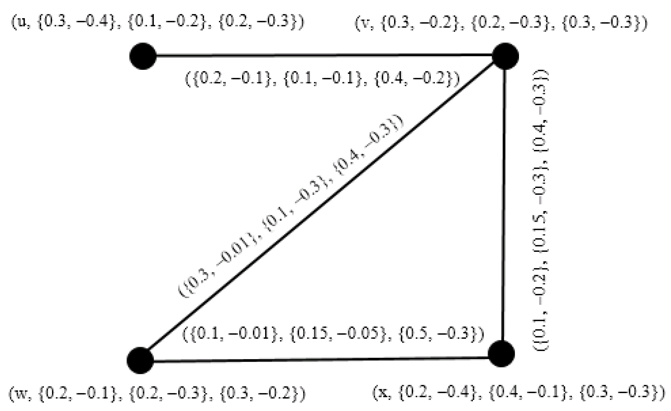
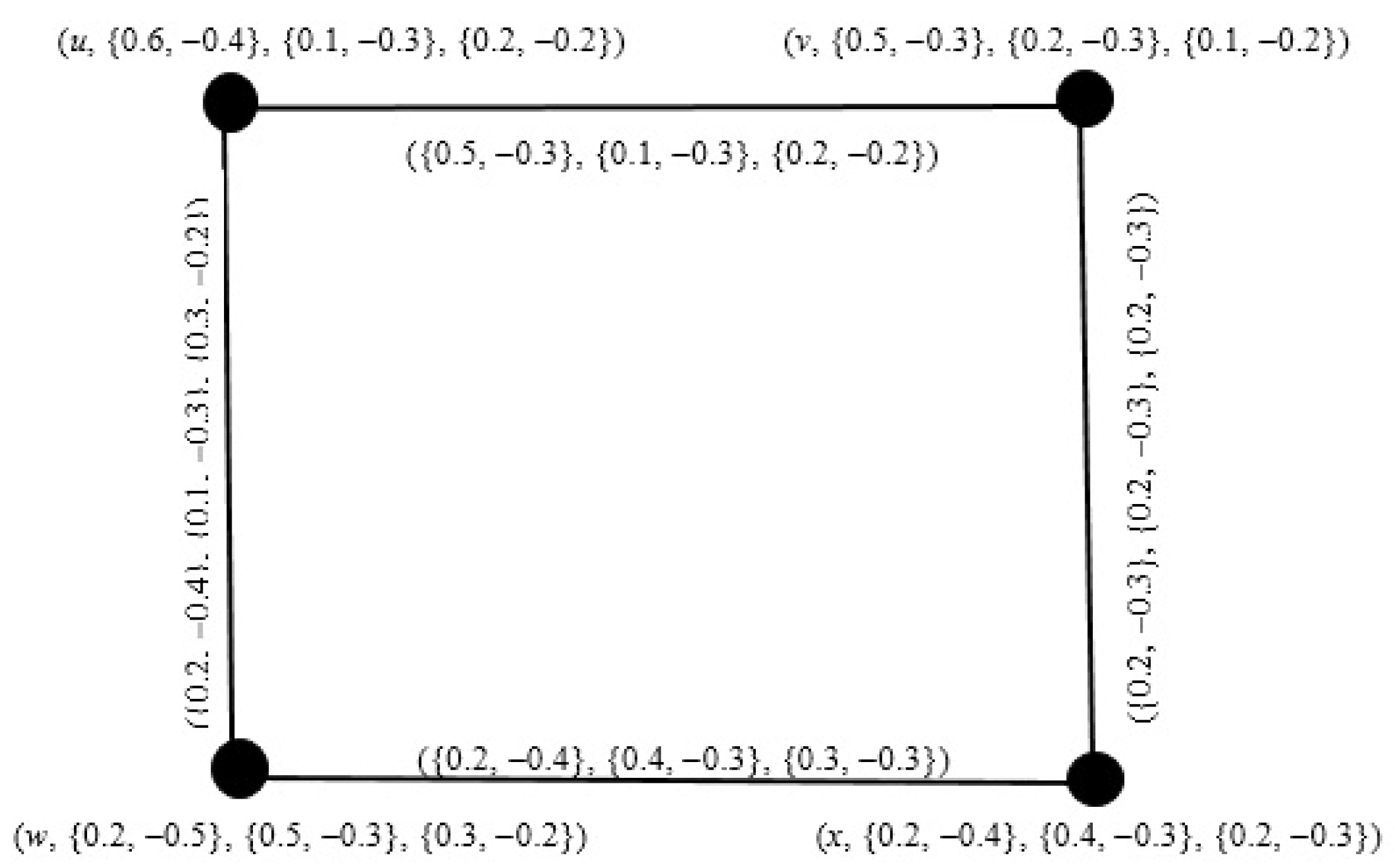
Let be a graph. A pair is said to be a bipolar picture fuzzy graph (BPPFG) on where , , , , , is a bipolar picture fuzzy set on V and , , , , , is a bipolar picture fuzzy set on such that for every edge ,
satisfying
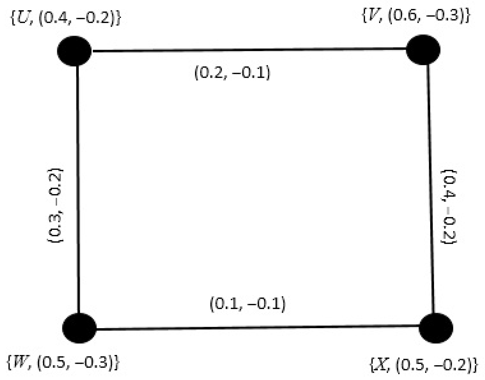
Example 1.
One can easily verify that the graphs shown in Figure 1a,b are BPPFGs.
Definition 18.
The order of a BPPFG is defined by , where
Definition 19.
The size of a BPPFG is denoted and defined by , where
Definition 20.
Let and be two graphs. Let be a BPPFG on , where , , , , , is a BPPFS on and , , , , , is a BPPFS on , respectively. Let be a BPPFG on , where , , , , , is a BPPFS on and , , , , , is a BPPFS on be the two BPPFGs. Then the operations union and intersection between J and K can be defined as
For any vertex u:
Case :
= max max min max min max:
Case :
= max max min max min max:
Case :
= max max min max min max:
Similarly, for any edge :
Case :
= max max min max min max:
Case :
= max max min max min max:
Case :
= max max min max min max:
For any vertex u:
Case :
= min max min max min :
Case :
= min max min max min :
Case :
= min max min max min :
Similarly, for any edge :
Case :
= min max min max min : .
Case :
= min max min max min : .
Case :
= min max min max min : .
Definition 21.
Let and be the two BPPFGs on and , respectively. Then the ring sum = ,−) of BPPFGs of and is the graph , where C = , , , , , is bipolar picture fuzzy set on and D = , , , , , is a bipolar picture fuzzy set on − satisfying the following conditions.
(A)
(B)
(C)
(D)
(E)
(F)
(G)
(H)
(I)
(J)
(K)
(L)
where represents an edge between the two vertices while , represent edges sets in and , respectively.
Theorem 1.
Ring sum of two BPPFGs is a BPPFG.
Proof.
Let us consider two BPPFGs and defined on crisp graphs and . Then, their ring sum = is BPPFG. Where , , , , , and , , , , , . Then we have the following cases.
Case 1:
If , then = , which is a BPPFS on . Additionally, if , then = , which is a BPPFS on .
Case 2:
If , then = , which is a BPPFS on Additionally, if , then = , which is a BPPFS on
Case 3:
If , then = , which is a BPPFS. Additionally, if , then = , which is BPPFR on
Similarly, we can show for all , , , , and , , , , . Since, , and are BPPFGs. Hence = G is a BPPFG. □
Proposition 1.
Let be a BPPFG on . Then = = H and = ∅ are BPPFGs.
Proof.
Let be a BPPFG on , where , , , , , is a BPPFS on V and , , , , , is a BPPFS on E, respectively. For , by Definition 20(1), we have
= max max min max min max: and
= max max min max min max:.
Thus, we have and . Hence
Similarly, for = (, ), by Definition 20(2), we have
= min max min max min : and
= min max min max min : .
Thus, and implies .
Finally, to prove = ∅. Let be any vertex, then by Definition (21) we have
Hence, = , ∀
Similarly, for any edge . Following Definition 21, we have
It implies = ∅, ∀ Thus, = ∅, which completes the proof. □
Definition 22.
The open neighbourhood degree of a vertex m of a BPPFG is deg(m) = , , , , , , where
= , =
= , =
= , =
Definition 23.
A vertex u in a BPPFG is said to be a busy vertex, if
Otherwise, it is a free vertex.
Definition 24.
The busy value of a vertex u of a BPPFG is defined by = , , , , , , where
represent the neighbors of u, the sum of the busy values of all vertices of H i.e., is said to be a busy value of a BPPFG H.
Definition 25.
The busy value of an edge of a BPPFG is defined by = , , , , , such that
Definition 26.
The set of sequence of different vertices , is the path p in a BPPFG such that , , and (, , ; .
Definition 27.
Two vertices u and v are connected by a path p i.e., of length l in a BPPFG . Then, , and are illustrated as follows.
Theorem 2.
Let be a BPPFG. If H contains a “” walk of length k, then H contains a “” path of length k.
3.1. Different Types of Products of Bipolar Picture Fuzzy Graphs
Definition 28.
The strong product of two BPPFGs , where , , , , , , , , , , and , where , , , , , , , , , , , where we take = ∅, is defined as
= (, , , , , , , , , , , ) of . Where E = : : ∪ : ,
and
= , = , = ,
= , = , = ,
for all . Similarly,
= , = , = ,
= , = ,
= , = ,
= , = .
Remark 1.
The strong product of two BPPFGs is always a BPPFG.
Definition 29.
The semi-strong product of two BPPFGs , where , , , , , , , , , , , with crisp graphs = and , where , , , , , , , , , , with crisp graph = , where we assume that = ∅, is defined to be the BPPFG = , with crisp graph such that ∪ , . Then
= min, = max for all
= min, = max for all
= max, = min for all
= min( and = min
= max and = max
= min and = min(
= max and = max
= max and = max
= min and = min.
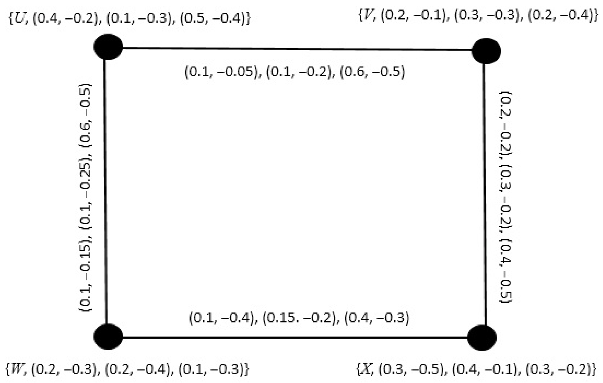
Example 2.
Let us consider two BPPFGs graphs given in Figure 1a,b. Then their semi-strong product is as follows.
= min, = max for all
= min, = max for all
= max, = min for all .
Consequently, for vertex u:
= min(0.6, 0.3) = 0.3, = max(−0.4, −0.5) = −0.4
= min(0.1, 0.5) = 0.1, = max(−0.3, −0.2) = −0.2
= max(0.2, 0.2) = 0.2, = min(−0.2, −0.3) = −0.3
(u, 0.3, −0.4, 0.1, −0.2, 0.2, −0.3)
Similarly, for vertex v, w and x:
(v, 0.3, −0.2, 0.2, −0.3, 0.3, −0.3), (w, 0.2, −0.1, 0.2, −0.3, 0.3, −0.2), (x, 0.2, −0.4, 0.4, −0.1, 0.3, −0.3)
Now edges of the semi−strong product of two graphs can be obtained by using , and of Definition 28
For an edge : (0.2, −0.1, 0.1, −0.1, 0.4, −0.2) For an edge : (0.1, −0.01, 0.15, −0.05, 0.5, −0.3)
For an edge : (0.3, −0.01, 0.1, −0.3, 0.4, −0.3) For an edge : (0.1, −0.2, 0.15, −0.3, 0.4, −0.3).
Definition 30.
The normal product of two BPPFGs = and with underlying crisp graphs = and = , respectively, is defined as a BPPFG G = = (, ) with underline crisp graph , where and )() : u = or v = x, ∪E = )() : ∈, with
= ∧, = ∨
= ∧, = ∨
= (∨), = ( ∧
for all
= ∧, = ∨
= ∧, = ∨
= (∨), = (∧
for all and
= ∧, = ∨
= ∧, = ∨
= (∨), = (∧
for all and
= ∧, = ∨
= ∧, = ∨
= (∨), = (∧
for all and .
Definition 31.
Let H = with underlying crisp graph = , where V = , E = be the normal product of two BPPFGs = and = with crisp graphs = and = , respectively. Then the degree of the vertex in V is denoted by d() = • (), •, •(), •(), •(), • () and is defined by
•() = ∧+∧ = ∧
•() = ∨+∨ = ∨
•() = ∧+∧ = ∧
•() = ∨+∨ = ∨
•() = ∨+∨ = ∨
•() = ∧+∧ = ∧.
Theorem 3.
Let = () and = () be two BPPFGs. If ≥, ≤, ≥, ≤, ≤, ≥ ≥, ≤, ≥, ≤, ≤, ≥ and ≥, ≤, ≥, ≤, ≤, ≥, then () = + .
3.2. Homomorphism of Bipolar Picture Fuzzy Graphs
Definition 32.
Let and be the two BPPFGs. A homomorphism f : → is the map f : → satisfying
(a) ,
(b) ,
(c) ,
(d) ,
(e) ,
(f) ,
for all , .
Definition 33.
Let and be the two BPPFGs. An isomorphism f : is a bijective mapping f : which satisfies
(a) = , =
(b) = , =
(c) = , =
(d) = , =
(e) = , =
(f) = , =
for all , .
Proposition 2.
The isomorphism between BPPFGs is an equivalence relation.
Definition 34.
Let and be the two BPPFGs. Then a weak isomorphism is a bijective map satifying
(a) h is a homomorphism.
(b) = , =
(c) = , =
(d) = , =
for all . Evidently, the co-weak isomorphism fixes only the weights of the vertices.
Definition 35.
Let be the two BPPFGs. The co-weak isomorphism is the bijective map h : which satisfies
(a) h is a homomorphism
(b) = , =
(c) = , =
(d) = , =
for all . Evidently, the co-weak isomorphism fixes only the weights of the edges.
Proposition 3.
Weak isomorphism between BPPFGs always induces a partial order relation.
Theorem 4.
Let be a BPPFG and Aut(G) be the set of all automorphisms of G. Then (Aut(G), ∘) forms a group.
Proof.
Let , , and let . Then
Thus, ∘∈ Aut(G). Similarly, one can easily prove that = ), where , , ∈ Aut(G). Additionally, we have the inverses for each Aut defined as = , = , = , = , = , = . Similarly, there exists e∈ Aut(G). Let ∘e = = e∘. = Aut(G) is the identity element. Hence (Aut(G), ∘) forms a group. □
Proposition 4.
Let be a BPPFG and Aut(H) be the set of all automorphisms of H. Let , , , , , ) be a BPPFS in Aut(H) defined by
for all , Aut(H). Then, , , , , , ) is a bipolar picture fuzzy group on Aut(H).
Proof.
Follows from Theorem 3. □
3.3. Complete and Strong Bipolar Picture Fuzzy Graphs
Definition 36.
A BPPFG of a graph , where , , , , , and , , , , , is called a complete bipolar picture fuzzy graph (complete BPPFG) if
for all .
Example 3.
One can easily verify that the graph shown in Figure 1a is a complete BPPFG.
Theorem 5.
Let and be two complete BPPFGs. Then their direct product is also a complete BPPFG.
Proof.
As we know that the strong product of BPPFGs is a BPPFG and each pair of vertices are adjacent, . Now, for all , since is complete
() = ∧ = ∧∧ = ∧
() = ∨ = ∨∨ = ∨
() = ∧ = ∧∧ = ∧
() = ∨ = ∨∨ = ∨
() = ∨ = ∨∨ = ∨
() = ∧ = ∧∧ = ∧
If , then
() = ∧ = ∧∧ = ∧
Similarly, one can easily verify that
If , then as and are complete
() = ∧ = ∧∧∧
Similarly, we can show that
Hence, is a complete BPPFG. □
Definition 37.
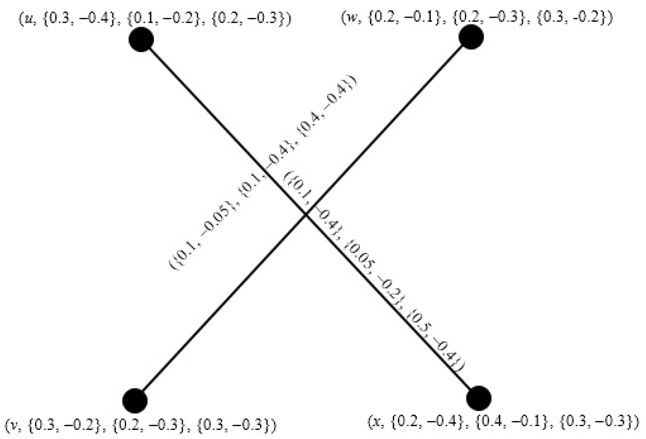
A BPPFG on a graph , where , , , , , and , , , , , is said to be a strong bipolar picture fuzzy graph (in short, BPPFG) if
for all .
Example 4.
The graph shown in Figure 3 is a strong BPPFG.
Remark 2.
Every complete BPPFG implies a strong BPPFG but the converse does not exist.
Definition 38.
The complement of a strong BPPFG of a graph , where , , , , , and , , , , , is a BPPFG = , of = , where = , , , , , and = , , , , , is defined by
for all , .
Theorem 6.
Let and be the two strong BPPFGs. Then is strong BPPFG.
Proof.
Let . Since and are strong BPPFGs, we have
(()) = ∧( = ∧∧∧ = (⊓)() ∧ (⊓)()
() = ∨( = ∨∨∨ = (⊓)() ∧ (⊓)()
(()) = ∧( = ∧∧∧ = (⊓)() ∧ (⊓)()
() = ∨( = ∨∨∨ = (⊓)() ∧ (⊓)()
(()) = ∨( = ∧∧∧ = )() ∨ (⊓)()
() = ∧( = ∧∧∧ = (⊓)() ∧ (⊓)(
□
4. Application
Modelling by using graphs has vast applications in various fields of computer science, mathematics, chemistry, physics, social sciences etc. Usually such types of models require more arrangements than merely the adjacencies among the vertices. In the study of social circuits, it is found that two people know each other i.e., if they are familiar (acquainted), or whether they are friends of each others (in the real world or in the virtual world such as Instagram) and so on. We can label each person in a particular group of people by a vertex u. There is an undirected edge between a vertex u and v if two people has a relationship with each other. In such type of graphs no multiple edges and usually no loops are needed. There is an edge between the vertices u and v when there is any acquaintanceship exists between them. In such graphs there does not exist any loop or multiple edges. In acquaintanceship graphs, the vertex (node) represents the level of acquaintanceship (how much a person is socialized or familiar/friendly) of a person while the the edge is the acquaintanceship between two persons in the social network. Since each vertex has equal importance in the classical graphs, it is not possible to graph the social networks model properly through them. In addition, all social units (individual or organization) present in social groups must be considered with equal importance in the classical graph theory. However, in the real life, the situation is different. Similarly, every edge (relationship) has an equal strength in the classical graphs. Moreover, in classical graphs it is assumed that the relationship between two social units are of equal strength, however, in real life it is not possible. Thus the acquaintance of the person has fuzzy boundary and hence can be better represented through the fuzzy graphs. In fuzzy acquaintanceship graph, each vertex represents the person and its membership value which reflects the strength of acquaintance of the person within the social group. Hence we present a fuzzy acquaintanceship graph, a bipolar fuzzy acquaintanceship and consequently a bipolar picture fuzzy acquaintanceship graph models to find out that how much the person is acquainted (social) within a group. Bipolar picture fuzzy acquaintanceship graph models would be more efficient to detect the symmetry or asymmetry existing between entities through the levels of acquaintanceships in social networks, computer networks etc.
4.1. Fuzzy Acquaintanceship Graph
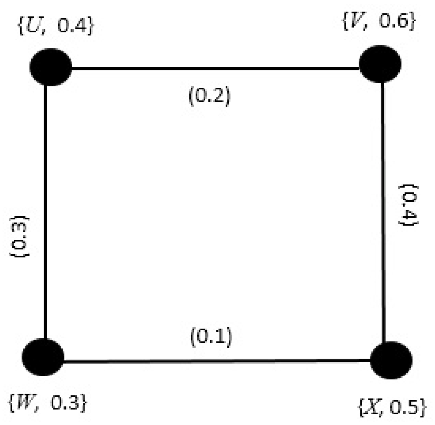
We take a fuzzy acquaintanceship graph of a social network which is shown in Figure 5. In which the nodes represent the degree of the level of acquaintance of a person within the social group. The degree of the level of acquaintance is expressed in its membership value. Degree of membership states that how much a person is acquainted e.g., X is acquainted within the group. The edges of a graph describe the acquaintanceship level of one person with the other person. The membership degree of edges can be considered in terms of positive percentage e.g., Y has acquaintanceship level with X and so.
4.2. Bipolar Fuzzy Acquaintanceship Graph
The acquaintanceship of a person may be positive or negative. Suppose if a person A and B belong to a social network but having not a good relationships between them then the acquaintanceship between them is negative. We can depict such circumstances through the bipolar fuzzy acquaintanceship graph. Consider a bipolar fuzzy acquaintanceship graph of a social group shown in Figure 6. In which the nodes are reflecting the degree of the level of acquaintanceship of a person belongs to a social group and the edges represent the degree of acquaintanceship levels among the persons. Degree of positive membership can be interpreted as how much a person acquainted and negative membership tells us that how much a person losses the the level of acquaintance, X has 50% level of acquaintance within the group but it loses 20% level in the same group. Edges of the graph reflect the acquaintance of one person with the other persons in the group. The positive and negative memberships degrees of edges describes the percentage of positive and negative acquaintance, for instance e.g., X is acquainted 10% with W and W is not acquainted 10% with X.
4.3. Bipolar Picture Fuzzy Acquaintanceship Graph
The degree of the acquaintanceship of a person is defined in terms of its membership (positive, negative), non-membership (positive, negative) and neutral membership (positive, negative) values. The degree of the membership (positive, negative) can be interpreted as a good acquaintanceship (gaining, losing). By a good acquaintanceship, we mean the acquaintance with intimacy. The degree of non-membership (positive, negative) can be interpreted as a bad acquaintanceship (gaining, losing). Bad acquaintanceship means acquaintance with ill-famed. The degree of neutral membership (positive, negative) represents that the person having a loose acquaintanceship (gaining, losing). By a loose acquaintanceship, we mean someone we do not know well enough but we probably see them around occasionally. In Figure 7, X gains (resp., loses) 30% (resp., 50%) good acquaintanceship, he gains 20% (resp., loses 10%) bad acquaintanceship but he gains (resp., loses) 30% (resp., loses 20%) loose acquaintanceship within the social group. On the other hands, the edges of a graph (Figure 7) reflect the acquaintanceship of one person with another person. The degree of a membership (positive and negative), non-membership (positive and negative) and neutral membership(positive and negative) of the edges can be interpreted as the percentage of good acquaintanceship (gaining, losing), bad acquaintanceship (gaining, losing) and non-acquaintanceships (gaining, losing). Furthermore, it is easy to verify that the values of the edges of a graph in Figure 7 are satisfying the below conditions.
Refer to the graph shown in Figure 7, we have
≤ min ⇒ ≤ min (0.4, 0.2) ⇒ 0.1 ≤ 0.2
≥ max ⇒ ≥ max (-0.2, -0.1) ⇒ −0.05 ≥ −0.1
≤ min ⇒ ≤ min (0.1, 0.3) ⇒ 0.1 ≤ 0.1
≥ max ⇒ ≥ max (-0.3, -0.3) ⇒ −0.2 ≥ −0.3
≥ max ⇒ ≥ max (0.2, 0.5) ⇒ 0.6 ≥ 0.5
≤ min ⇒ ≤ min (−0.4, −0.4) ⇒ −0.5 ≤ −0.4.
Hence by doing same calculations for the other vertices and edges of the graph shown in Figure 7, it is easy to verify that the graph given in Figure 7 is a bipolar picture fuzzy acquaintanceship graph. Similarly, by the values of vertices and edges, one can easily deduce that the graph in Figure 7 is asymmetric.
5. Conclusions
Fuzzy graphs theory plays a significant role in modeling many real world problems containing uncertainties in different fields such as decision making theory, computer science, optimization problems, data analysis, networking etc. In this perspective, a number of generalizations of fuzzy graph have been introduced to deal with the difficult and complex real life problems. The picture fuzzy set is a direct extension of both the fuzzy sets and intuitonistic fuzzy sets. Bipolar fuzzy set is another generalized form of fuzzy set which is also an effective tool for the multiagent decision analysis. The main goal of this manuscript is to initiate the concepts of bipolar picture fuzzy graph and its different characterizations. In this article, first we propose the definition of bipolar picture fuzzy graphs based on the bipolar picture fuzzy relation. In this article, we have introduced the terms bipolar picture fuzzy graphs, complete bipolar picture fuzzy graphs and strong bipolar picture fuzzy graphs along with their several fundamental properties. For the sake of investigations, we have introduced and applied numerous operations like union, intersection, complement, ring sum etc. on bipolar picture fuzzy graphs. We also introduce different types of products of bipolar picture fuzzy graphs like semi-strong product, direct product, normal products etc. Several other terms such as order and size, path neighborhood degrees, busy values of vertices and edges of bipolar picture fuzzy graphs are also studied. These terminologies also laid the foundation for the discussion of regular bipolar picture fuzzy graphs. Furthermore, we also discuss isomorphisms, weak and co-weak isomorphisms and automorphisms of bipolar picture fuzzy graphs. During this, we have proved that the set of all automorphisms of a bipolar picture fuzzy graph forms a group. Finally, we construct a bipolar picture fuzzy acquaintanceship graph which reflects the importance of our theoretical results produced in this article. Evidently, the network modelled through a bipolar picture fuzzy acquaintanceship graph shown in Figure 7 has no any symmetry. However, we can also model a symmetric relation through the bipolar picture fuzzy acquaintanceship graph. On the same patterns, one could express collaboration graph, computer networking, social networking, web graphs in the frame of bipolar picture fuzzy graphs. In general, numbers of applications of bipolar fuzzy graphs and picture fuzzy graphs have been explored in different fields of social, natural and computer sciences. Evidently, bipolar picture fuzzy graphs would be an important tool to deal with real world problems containing uncertainties. Finally, one can extend this work by introducing bipolar interval-valued picture fuzzy graphs.
Author Contributions
Conceptualization, W.A.K. and B.A.; methodology, B.A., W.A.K. and A.T.; validation, B.A., A.T. and W.A.K.; formal analysis, B.A. and W.A.K.; investigation, B.A. and A.T.; writing—original draft preparation, W.A.K.; writing—review and editing, B.A. and A.T.; supervision, W.A.K.; funding acquisition, W.A.K., B.A. and A.T. All authors have read and agreed to the published version of the manuscript.
Funding
This research received no external funding.
Data Availability Statement
Not Applicable.
Conflicts of Interest
The authors declare no conflict of interest.
References
- Zadeh, L.A. Fuzzy sets. Inf. Con. 1965, 8, 338–353. [Google Scholar] [CrossRef] [Green Version]
- Bustince, H.; Burillo, P. Correlation of interval-valued intuitionistic fuzzy sets. Fuzzy Sets Syst. 1995, 74, 237–244. [Google Scholar] [CrossRef]
- Khalil, A.M.; Li, S.G.; Garg, H.; Li, H.; Ma, S. New operations on interval-valued picture fuzzy set, interval-valued picture fuzzy soft set and their applications. IEEE Access 2019, 7, 51236–51253. [Google Scholar] [CrossRef]
- Zadeh, L.A. The concept of a linguistic variable and its application to approximate reasoning I. Inform. Sci. 1975, 8, 199–249. [Google Scholar] [CrossRef]
- Zhang, W.-R. Bipolar fuzzy sets and relations: A computational framework for cognitive modeling and multiagent decision analysis. In Proceedings of the First International Joint Conference of the North American Fuzzy Information Processing Society Biannual Conference, the Industrial Fuzzy Control and Intellige, San Antonio, TX, USA, 18–21 December 1994; pp. 305–309. [Google Scholar]
- Mandal, W.A. Bipolar pythagorean fuzzy sets and their application in Multi-attribute decision making problems. Ann. Data Sci. 2021, 1–33. [Google Scholar]
- Dudziak, U.; Pea, B. Equivalent bipolar fuzzy relations. Fuzzy Sets Syst. 2010, 161, 234–253. [Google Scholar] [CrossRef]
- Atanassov, K. Intuitionistic fuzzy sets. Fuzzy Sets Syst. 1986, 20, 87–96. [Google Scholar] [CrossRef]
- Cuong, B.C. Picture fuzzy sets. J. Comput. Sci. Cybern. 2014, 30, 409–420. [Google Scholar]
- Bo, C.; Zhang, X. New operations of picture fuzzy relations and fuzzy comprehensive evaluation. Symmetry 2017, 9, 268. [Google Scholar] [CrossRef] [Green Version]
- Cuong, B.C.; Pham, V.H. Some fuzzy logic operators for picture fuzzy sets. In Proceedings of the 2015 Seventh International Conference on Knowledge and Systems Engineering (KSE), Ho Chi Minh City, Vietnam, 8–10 October 2015; pp. 132–137. [Google Scholar] [CrossRef]
- Rosenfeld, A. Fuzzy graphs. In Fuzzy Sets and Their Applications to Cognitive and Decision Processes; Zadeh, L.A., Fu, K.S., Shimura, M., Eds.; Academic Press: New York, NY, USA, 1975; pp. 77–95. [Google Scholar]
- Bhattacharya, P. Some remarks on fuzzy graphs. Pattern Recognit. Lett. 1987, 6, 297–302. [Google Scholar] [CrossRef]
- Mordeson, J.N.; Peng, C.S. Operations on fuzzy graphs. Inform. Sci. 1994, 79, 159–170. [Google Scholar] [CrossRef]
- Sunitha, M.S.; Vijayakumar, A. Complement of a fuzzy graph. Indian J. Pure Appl. Math. 2002, 33, 1451–1464. [Google Scholar]
- Akram, M.; Dudec, W.A. Interval-valued fuzzy graphs. Comput. Math. Appl. 2011, 61, 289–299. [Google Scholar] [CrossRef] [Green Version]
- Shannon, A.; Atanassov, K.T. A first step to a theory of the intuitionistic fuzzy graphs. In Proceedings of the First Workshop on Fuzzy Based Expert Systems, Sofia, Bulgaria, 28–30 September 1994; pp. 59–61. [Google Scholar]
- Parvathi, R.; Karunambigai, M.G.; Atanassov, K.T. Operations on intuitionistic fuzzy graphs. In Proceedings of the 2009 IEEE International Conference on Fuzzy Systems, Jeju, Korea, 20–24 August 2009; pp. 1396–1401. [Google Scholar]
- Yaqoob, N.; Gulistan, M.; Kadry, S.; Wahab, H.A. Complex intuitionistic fuzzy graphs with application in cellular network provider companies. Mathematics 2019, 7, 35. [Google Scholar] [CrossRef] [Green Version]
- Akram, M. bipolar fuzzy graphs. Inform. Sci. 2011, 181, 5548–5564. [Google Scholar] [CrossRef]
- Yang, H.L.; Li, S.G.; Yang, W.H.; Lu, Y. Notes on a Bipolar fuzzy graphs. Inform. Sci. 2013, 242, 113–121. [Google Scholar] [CrossRef]
- Talebi, A.A.; Rashmanlou, H. Complement and isomorphism on bipolar fuzzy graphs. Fuzzy Inf. Eng. 2014, 6, 505–522. [Google Scholar] [CrossRef] [Green Version]
- Ghorai, G.; Pal, M. A note on Regular bipolar fuzzy graphs. Neural Computing and Applications 21 (1)(2012) 197–205. Neural Comput. Appl. 2018, 30, 1569–1572. [Google Scholar] [CrossRef]
- Poulik, S.; Ghorai, G. Certain indices of graphs under bipolar fuzzy environment with applications. Soft Comput. 2020, 24, 5119–5131. [Google Scholar] [CrossRef]
- Ghorai, G. Characterization of regular bipolar fuzzy graphs. Afr. Mat. 2021, 32, 1043–1057. [Google Scholar] [CrossRef]
- Zuo, C.; Pal, A.; Dey, A. New concepts of picture fuzzy graphs with application. Mathematics 2019, 7, 470. [Google Scholar] [CrossRef] [Green Version]
- Das, S.; Ghora, G. Analysis of road map design based on multi-graph with picture fuzzy information. Int. J. Appl. Comput. Math. 2020, 6, 1–17. [Google Scholar] [CrossRef]
- Xiao, W.; Dey, A.; Son, L.H. A Study on Regular Picture Fuzzy Graph with Applications in Communication Networks. J. Intell. Fuzzy Syst. 2020, 39, 3633–3645. [Google Scholar] [CrossRef]
- Koczy, L.T.; Jan, N.; Mahmood, T.; Ullah, K. Analysis of social networks and Wi-Fi networks by using the concept of picture fuzzy graphs. Soft Comput. 2020, 24, 16551–16563. [Google Scholar] [CrossRef]
- Amanathulla, S.; Bera, B.; Pal, M. Balanced picture fuzzy graph with application. Artif. Intell. Rev. 2021, 1–27. [Google Scholar]
- Diestel, R. Graph Theory. USA; Springer: Berlin/Heidelberg, Germany, 2000. [Google Scholar]
- Zimmermann, H.J. Fuzzy Set Theory and Its Applications; Springer Science & Business Media: Berlin/Heidelberg, Germany, 2011. [Google Scholar]
- Zhang, W.-R. (Yin)(Yang) bipolar fuzzy sets. In Proceedings of the 1998 IEEE International Conference on Fuzzy Systems Proceedings, IEEE World Congress on Computational Intelligence (Cat. No. 98CH36228), Anchorage, AK, USA, 4–9 May 1998; pp. 835–840. [Google Scholar]
- Samanta, S.; Pal, M. Some more results on bipolar fuzzy sets and bipolar fuzzy intersection graphs. J. Fuzzy Math. 2014, 22, 253–262. [Google Scholar]
- Ezhilmaran, D.; Sankar, K. Morphism of bipolar intuitionistic fuzzy graphs. J. Discrete Math. Sci. Cryptogr. 2015, 18, 605–621. [Google Scholar] [CrossRef]
- Khan, W.A.; Faiz, K.; Taouti, A. Bipolar picture fuzzy sets and relations with applications. Submiited.
Figure 1.
Bipolar picture fuzzy graph.

Figure 2.
Semi-strong product of bipolar picture fuzzy graphs shown in Figure 1a,b.
Figure 2.
Semi-strong product of bipolar picture fuzzy graphs shown in Figure 1a,b.

Figure 3.
Strong bipolar picture fuzzy graph.

Figure 4.
Complement of a strong bipolar picture fuzzy graph given in Figure 3.
Figure 4.
Complement of a strong bipolar picture fuzzy graph given in Figure 3.

Figure 5.
Fuzzy acquaintanceship graph.

Figure 6.
Bipolar fuzzy acquaintanceship graph.

Figure 7.
Bipolar picture fuzzy acquaintanceship graph.

Publisher’s Note: MDPI stays neutral with regard to jurisdictional claims in published maps and institutional affiliations. |
© 2021 by the authors. Licensee MDPI, Basel, Switzerland. This article is an open access article distributed under the terms and conditions of the Creative Commons Attribution (CC BY) license (https://creativecommons.org/licenses/by/4.0/).
Share and Cite
MDPI and ACS Style
Khan, W.A.; Ali, B.; Taouti, A. Bipolar Picture Fuzzy Graphs with Application. Symmetry 2021, 13, 1427. https://0-doi-org.brum.beds.ac.uk/10.3390/sym13081427
AMA Style
Khan WA, Ali B, Taouti A. Bipolar Picture Fuzzy Graphs with Application. Symmetry. 2021; 13(8):1427. https://0-doi-org.brum.beds.ac.uk/10.3390/sym13081427
Chicago/Turabian StyleKhan, Waheed Ahmad, Babir Ali, and Abdelghani Taouti. 2021. "Bipolar Picture Fuzzy Graphs with Application" Symmetry 13, no. 8: 1427. https://0-doi-org.brum.beds.ac.uk/10.3390/sym13081427
Note that from the first issue of 2016, this journal uses article numbers instead of page numbers. See further details here.