The Scalar Mean Chance and Expected Value of Regular Bifuzzy Variables

Abstract

As a natural extension of the fuzzy variable, a bifuzzy variable is defined as a mapping from a credibility space to the collection of fuzzy variables, which is an appropriate tool to model the two-fold fuzzy phenomena. In order to enrich its theoretical foundation, this paper explores some important measures for regular bifuzzy variables, the most commonly used type of bifuzzy variables. Firstly, we introduce the regular bifuzzy variables’ mean chance measure and some properties, including self-duality and its calculation formulas. Furthermore, we also investigate the mean chance distribution for strictly monotone functions of regular bifuzzy variables based on the proposed operational law. Finally, we present the expected value operator as well as equivalent analytical formulas of the expected value of regular bifuzzy variables and their strictly monotone functions.

1. Introduction

Since the fuzzy set theory was proposed by Zadeh [1], it has been widely adopted in a variety of academic research and real-world applications to deal with the imprecision implied in judgments, expertise, and linguistic descriptions. As this kind of research was explored in depth, scholars realized that the information of the fuzzy set cannot be accurately obtained in many cases. As a result, they paid close attention to the extensions on the fuzzy set. On the one hand, the incomplete information on the degree of membership attracted attention from scholars, and some well-accepted tools were developed to handle this type of fuzziness, such as the type 2 fuzzy set by Zadeh [2] in 1975, the twofold fuzzy set by Dubois and Prade [3] in 1983, and the intuitionistic fuzzy set by Atanassov [4] in 1986. On the other hand, the scenario with imprecise information on objects of the universal has also received attention. In 2002, Liu [5] initially put forward a new concept, the bifuzzy variable, as a function from a possibility space to the fuzzy variables set; moreover, some important attributes were also defined. As a continuation of [5], Zhou and Liu [6,7] investigated some mathematical properties of this kind of variable, such as chance distribution and expected value operator. Afterwards, Qin and Li [8] gave and proved a sufficient and necessary condition for the chance distribution of the bifuzzy variable.

In addition to theoretical studies, scholars have also considered their research under the bifuzzy environment because such complex uncertainty has extensively existed in practical problems. Xu and Yan [9] developed a multi-objective integer model under the bifuzzy environment to handle a vendor selection problem for material supply in large-scale water conservancy and hydro-power construction projects. Both Chakraborty et al. [10] and Bera et al. [11] investigated the multi-product production-inventory models with bifuzzy parameters. Deng and Qiu [12,13] proposed the bifuzzy discrete event systems and established the supervisory control theories on this type of system under different observation levels successively. Taib et al. [14] formulated a group decision-making model on the basis of conflicting bifuzzy sets and applied it in flood control projects. Shi et al. [15] introduced a novel bifuzzy scheduling model, in order to deal with two-fold uncertainties existed in re-manufacturing. These studies illustrate the wide presence of the bifuzzy phenomenon in real-world applications.

However, due to the insufficient mathematical properties of the bifuzzy variable, its development and popularization have been constrained. Hence, in this research, we pay particular attention to the regular bifuzzy variables and investigate their mean chance and expected value. The main contributions are as follows. On the one hand, we not only study the mean chance measure of regular bifuzzy variables but also propose the operational law for formulating the mean chance distribution of strictly monotone functions of regular bifuzzy variables. On the other hand, we give theorems and equivalent analytical formulas to explicitly and directly compute the expected value of regular bifuzzy variables and their strictly monotone functions.

The rest of this paper is organized as follows. Section 2 recalls some fundamental concepts of fuzzy and bifuzzy variables and defines the concept of regular bifuzzy variables. Section 3 presents the mean chance measure and discusses its self-duality. In this section, we also propose the operational law for the strictly monotone function of regular bifuzzy variables. In Section 4, the calculations of the expected value of regular bifuzzy variables and their strictly monotone functions are given. The main findings are summarized in Section 5.

2. Fundamental Concepts

In order to measure the regular bifuzzy events, we state some important preliminaries and definitions about fuzzy and bifuzzy variables in the following.

2.1. Fuzzy Variables

To begin with, based upon the possibility theory, the credibility space introduced by Liu [16] is reviewed here.

Definition 1.

(Liu [16]) Suppose that Θ symbolizes a nonempty set, $\mathcal{P}\left(\mathsf{\Theta }\right)$ stands for the power set of Θ, and $\mathrm{Cr}$ represents the credibility measure, such that $\mathrm{Cr}\{\varnothing \}=0$, and $\mathrm{Cr}\left\{\mathsf{\Theta }\right\}=1$. Then, the triplet $(\mathsf{\Theta },\mathcal{P}(\mathsf{\Theta }),\mathrm{Cr})$ is called a credibility space.

Definition 2.

(Liu [16]) Suppose that the triplet $(\mathsf{\Theta },\mathcal{P}(\mathsf{\Theta }),\mathrm{Cr})$ represents a credibility space. Then, a fuzzy variable $\tilde{\tau }$ can be regarded as a function from this space to the set of real numbers.

Definition 3.

(Zadeh [1,17] and Liu and Liu [18]) Suppose that $\tilde{\tau }$ is a fuzzy variable. If the membership function of $\tilde{\tau }$ is given as ${\mu }_{\tilde{\tau }}$, then, to mathematically describe the fuzzy event $\{\tilde{\tau }\in \mathbb{B}\}$, where $\mathbb{B}$ is referred to any Borel set of $\mathbb{R}$, the possibility, necessity, and credibility measures can be written, respectively, as

$$\begin{array}{c}\mathrm{Pos}\{\tilde{\tau }\in \mathbb{B}\}={\sup }_{x\in \mathbb{B}}{\mu }_{\tilde{\tau }}\left(x\right),\hfill \\ \mathrm{Nec}\{\tilde{\tau }\in \mathbb{B}\}=1-{\sup }_{x\in {\mathbb{B}}^c}{\mu }_{\tilde{\tau }}\left(x\right),\hfill \\ \mathrm{Cr}\{\tilde{\tau }\in \mathbb{B}\}=(\mathrm{Pos}\{\tilde{\tau }\in \mathbb{B}\}+1-\mathrm{Nec}\{\tilde{\tau }\in \mathbb{B}\})/2.\hfill \end{array}$$

(1)

Definition 4.

(Liu [19]) Suppose that $\tilde{\tau }$ is a fuzzy variable. Then, the credibility distribution of $\tilde{\tau }$ is defined as

$${\mathsf{{\rm Y}}}_{\tilde{\tau }}\left(y\right)=\mathrm{Cr}\{\theta \in \mathsf{\Theta }|\tilde{\tau }\left(\theta \right)\le y\},\forall y\in \mathbb{R}.$$

(2)

Meanwhile, since the LR-type fuzzy number was initially proposed by Dubios and Prade [20], it has been adopted to various practical programmings. Subsequently, based on this special fuzzy number, the following definitions are presented.

Definition 5.

(Dubios and Prade [20,21]) Suppose that two shape functions are described as $L(·)$ and $R(·)$. If $L(·)$ (and $R(·)$) is a function that satisfies

(i) 

$L\left(0\right)=1;$

(ii) 

$L\left(x\right)<1,\forall x>0;$

(iii) 

$L\left(x\right)>0,\forall x<1;$

(iiii) 

$L\left(1\right)=0or\left[L\right(x)>0,\forall xandL(+\infty )=0];$

(iiiii) 

$L\left(x\right)$ is nonincreasing on $[0,+\infty )$,

and the fuzzy number $\tilde{\tau }$ has the following membership function

$${\mu }_{\tilde{\tau }}\left(x\right)=\left\{\begin{array}{cc}{\displaystyle L\left(\frac{b-x}{\iota }\right)},\hfill & \mathrm{if}x\le b\hfill \\ {\displaystyle R\left(\frac{x-b}{\upsilon }\right)},\hfill & \mathrm{if}x>b,\hfill \end{array}\right.$$

(3)

where b is called the peak of $\tilde{\tau }$ with ${\mu }_{\tilde{\tau }}\left(b\right)=1$, and ι and υ are called the left and right spreads with $\iota >0$ and $\upsilon >0$, respectively, then $\tilde{\tau }$ is said to be an LR-type fuzzy number. Symbolically, $\tilde{\tau }$ is written as ${(b,\iota ,\upsilon )}_{LR}$.

Example 1.

If a triangular fuzzy number $\tilde{\tau }$ is described as $\mathcal{T}(a_1,a_2,a_3)$ with real numbers $a_1<a_2<a_3$, and the shape functions satisfy that $L\left(x\right)=R\left(x\right)=max\{0,1-x\}$, then the membership function of $\tilde{\tau }$ is presented as

$${\mu }_{\tilde{\tau }}\left(x\right)=\left\{\begin{array}{cc}{\displaystyle \frac{x-a_1}{a_2-a_1}},\hfill & \mathrm{if}{a}_1<x\le a_2\hfill \\ {\displaystyle \frac{a_3-x}{a_3-a_2}},\hfill & \mathrm{if}{a}_2<x\le a_3\hfill \\ {\displaystyle 0},\hfill & \mathrm{otherwise}.\hfill \end{array}\right.$$

(4)

Example 2.

If an exponential fuzzy number $\tilde{\tau }$ is described as $\mathcal{E}(m,p,p)$ with real number $p>0$, and the shape functions satisfy $L\left(x\right)=R\left(x\right)=e^{-x}$, then the membership function of $\tilde{\tau }$ is presented as

$${\mu }_{\tilde{\tau }}\left(x\right)=\left\{\begin{array}{cc}{\displaystyle e^{-\frac{m-x}{p}}},\hfill & \mathrm{if}x\le m\hfill \\ {\displaystyle e^{-\frac{x-m}{q}}},\hfill & \mathrm{if}x>m.\hfill \end{array}\right.$$

(5)

Theorem 1.

(Zhou et al. [22]) Suppose that $\tilde{\tau }$ is an LR-type fuzzy variable. If the credibility distribution of $\tilde{\tau }$ is not only strictly increasing but continuous on its support, then $\tilde{\tau }$ is called a regular LR fuzzy variable.

In the rest of this paper, for convenience, the triplet ${(b,\iota ,\upsilon )}_{LR}$, whose elements are defined in Definition 5, refers to a regular LR fuzzy variable $\tilde{\tau }$. Generally, if $\tilde{\tau }$ has the same shape functions (i.e., $L(·)=R(·)$) and same left and right spreads (i.e., $\iota =\upsilon$), we may call it symmetric, which is a well-used type applied in mathematical formulations of fuzzy programmings.

Remark 1.

Clearly, for Example 1, the credibility distribution of $\tilde{\tau }$ can be deduced via its membership function according to Zhou et al. [22]. Thus, following from Definition 4 and the decreasing shape functions $L(·)$ and $R(·)$, the corresponding continuous and strictly increasing credibility distribution is obtained. Analogously, the same conclusions can be drawn for Example 2. Thus, these two LR-type fuzzy variables are obviously regular.

The credibility distributions and their inverse functions, named inverse credibility distributions, of the triangular fuzzy number and the exponential fuzzy variable are developed in Examples 3 and 4.

Example 3.

If a triangular fuzzy number $\tilde{\tau }$ is described by $\mathcal{T}(a_1,a_2,a_3)$, then its credibility distribution ${\mathsf{{\rm Y}}}_{\tilde{\tau }}$ and inverse credibility distribution ${\mathsf{{\rm Y}}}_{\tilde{\tau }}^{-1}$ are given as

$${\mathsf{{\rm Y}}}_{\tilde{\tau }}\left(y\right)=\left\{\begin{array}{cc}{\displaystyle 0},\hfill & \mathrm{if}y\le a_1\hfill \\ {\displaystyle 0.5\frac{y-a_1}{a_2-a_1}},\hfill & \mathrm{if}{a}_1<y\le a_2\hfill \\ {\displaystyle 1-0.5\frac{a_3-y}{a_3-a_2}},\hfill & \mathrm{if}{a}_2<y\le a_3\hfill \\ {\displaystyle 1},\hfill & \mathrm{if}y>a_3,\hfill \end{array}\right.$$

(6)

and

$${\mathsf{{\rm Y}}}_{\tilde{\tau }}^{-1}\left(\beta \right)=\left\{\begin{array}{cc}{\displaystyle a_1+2\beta (a_2-a_1)},\hfill & \mathrm{if}0<\beta \le 0.5\hfill \\ {\displaystyle (2-2\beta )a_2+(2\beta -1)a_3},\hfill & \mathrm{if}0.5<\beta <1.\hfill \end{array}\right.$$

(7)

Example 4.

If an exponential fuzzy number $\tilde{\tau }$ is described by $\mathcal{E}(m,p,p)$, then its credibility distribution ${\mathsf{{\rm Y}}}_{\tilde{\tau }}$ and inverse credibility distribution ${\mathsf{{\rm Y}}}_{\tilde{\tau }}^{-1}$ are given as

$${\mathsf{{\rm Y}}}_{\tilde{\tau }}\left(y\right)=\left\{\begin{array}{cc}{\displaystyle 0.5e^{-\frac{m-y}{p}}},\hfill & \mathrm{if}y\le m\hfill \\ {\displaystyle 1-0.5e^{-\frac{y-m}{p}}},\hfill & \mathrm{if}y>m,\hfill \end{array}\right.$$

(8)

and

$${\mathsf{{\rm Y}}}_{\tilde{\tau }}^{-1}\left(\beta \right)=\left\{\begin{array}{cc}{\displaystyle m+pln\left(2\beta \right)},\hfill & \mathrm{if}0<\beta \le 0.5\hfill \\ {\displaystyle m-pln(2-2\beta )},\hfill & \mathrm{if}0.5<\beta <1.\hfill \end{array}\right.$$

(9)

Apparently, note that for the triangular fuzzy number defined in Example 3, when $a_2=0.5(a_1+a_3)$, it is said to be symmetric. Meanwhile, by virtue of the parametric form of an exponential fuzzy number, the variable defined in Example 4 is also absolutely a symmetric regular LR fuzzy variable.

2.2. Bifuzzy Variables

In addition, several definitions of extension of the fuzzy variable have been proposed aiming at describing the two-fold uncertain phenomena, such as the bifuzzy variable, type-2 fuzzy variable, intuitionistic fuzzy variable, etc. In this paper, the concept of the bifuzzy variable introduced by Liu [6] is adopted for further study, which is shown as follows.

Definition 6.

(Liu [19]) Suppose that the triplet $(\mathsf{\Theta },\mathcal{P}(\mathsf{\Theta }),\mathrm{Cr})$ represents a credibility space. Then, a bifuzzy variable $\widetilde{\tilde{\mathsf{\kappa }}}$ can be regarded as a function from this space to the collection of fuzzy variables.

Remark 2.

Generally speaking, we may view $\widetilde{\tilde{\mathsf{\kappa }}}$ as a fuzzy variable $\tilde{\mathsf{\kappa }}$ defined on the universal collection of fuzzy variables. For the sake of convenience, $\tilde{\mathsf{\kappa }}$ is called a primary fuzzy number, and for each $\theta \in \mathsf{\Theta }$, $\widetilde{\tilde{\mathsf{\kappa }}}\left(\theta \right)$ is called a secondary fuzzy number. Therefore, the set of all secondary fuzzy numbers is exactly the above universal collection.

Example 5.

If ${\tilde{\tau }}_i$ is a fuzzy variable and ${\nu }_i$ is a real-valued number in $[0,1]$, $i=1,2,\cdots ,m$ and ${\nu }_1\vee {\nu }_2\vee \cdots \vee {\nu }_m=1$, then the function

$$\widetilde{\tilde{\mathsf{\kappa }}}=\left\{\begin{array}{cc}{\displaystyle {\tilde{\tau }}_1},\hfill & \mathrm{with}\mathrm{possibility}{\nu }_1\hfill \\ {\displaystyle {\tilde{\tau }}_2},\hfill & \mathrm{with}\mathrm{possibility}{\nu }_2\hfill \\ {\displaystyle \cdots }\hfill \\ {\displaystyle {\tilde{\tau }}_m},\hfill & \mathrm{with}\mathrm{possibility}{\nu }_m,\hfill \end{array}\right.$$

(10)

is obviously a bifuzzy variable according to Definition 6.

Example 6.

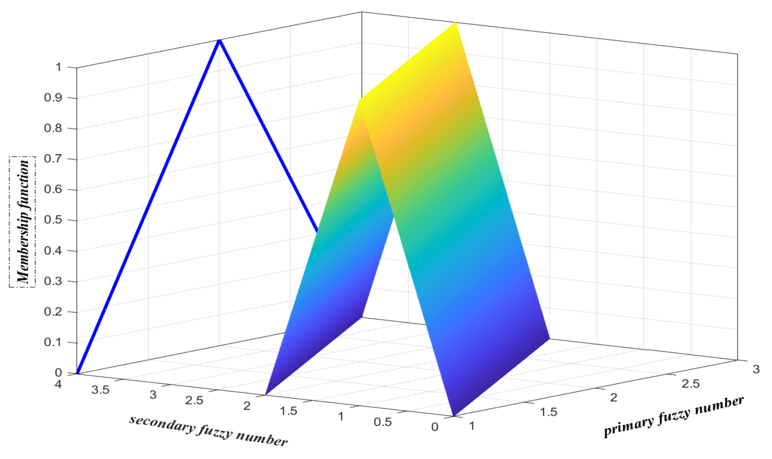
If a variable $\widetilde{\tilde{\mathsf{\kappa }}}$ is given as $\mathcal{T}(\tilde{\mathsf{\kappa }}-\iota ,\tilde{\mathsf{\kappa }},\tilde{\mathsf{\kappa }}+\upsilon )$, where $\tilde{\mathsf{\kappa }}$ represents a triangular fuzzy number, denoted as $\mathcal{T}(a_1,a_2,a_3)$, then $\widetilde{\tilde{\mathsf{\kappa }}}$ is also a bifuzzy variable. For example, if we take $\iota =\upsilon =1$ (i.e., $\widetilde{\tilde{\mathsf{\kappa }}}=\mathcal{T}(\tilde{\mathsf{\kappa }}-1,\tilde{\mathsf{\kappa }},\tilde{\mathsf{\kappa }}+1)$) and $a_1=1,a_2=2,a_3=3$ (i.e., $\tilde{\mathsf{\kappa }}=\mathcal{T}(1,2,3)$), then the interval $[0,4]$ is absolutely the domain of $\widetilde{\tilde{\mathsf{\kappa }}}$. Furthermore, the sketch map of the bifuzzy variable $\widetilde{\tilde{\mathsf{\kappa }}}$ is depicted in Figure 1, where the membership function of the primary fuzzy number is described by the blue line, and the membership functions of secondary fuzzy numbers are shown on the three-dimensional graph.

Definition 7.

(Liu [6]) Suppose that $\widetilde{\tilde{\mathsf{\kappa }}}$ is a bifuzzy variable. Then, for any $x\in \mathbb{R}$, the primitive chance of the bifuzzy event that $\widetilde{\tilde{\mathsf{\kappa }}}$ takes a value not larger than x, i.e., $\{\widetilde{\tilde{\mathsf{\kappa }}}\le x\}$, is a function from $(0,1]$ to $[0,1]$, defined as

$$\mathrm{Ch}\{\widetilde{\tilde{\mathsf{\kappa }}}\le x\}\left(\alpha \right)=\sup \left\{\beta \left|\mathrm{Cr}\right\{\theta \in \mathsf{\Theta }|\mathrm{Cr}\{\widetilde{\tilde{\mathsf{\kappa }}}\left(\theta \right)\le x\}\ge \beta \}\ge \alpha \right\}.$$

(11)

Definition 8.

(Liu [19]) Suppose that $\widetilde{\tilde{\mathsf{\kappa }}}$ is a bifuzzy variable. Then, the expected value of $\widetilde{\tilde{\mathsf{\kappa }}}$ is defined as

$$E\left[\widetilde{\tilde{\mathsf{\kappa }}}\right]={\int }_0^{+\infty }\mathrm{Cr}\left\{\theta \in \mathsf{\Theta }\left|E\right[\widetilde{\tilde{\mathsf{\kappa }}}\left(\theta \right)]\ge x\right\}\mathrm{d}x-{\int }_{-\infty }^0\mathrm{Cr}\left\{\theta \in \mathsf{\Theta }\left|E\right[\widetilde{\tilde{\mathsf{\kappa }}}\left(\theta \right)]\le x\right\}\mathrm{d}x,$$

(12)

provided that at least one of the two integrals is finite.

2.3. Regular Bifuzzy Variables

On the foundation of the above definitions, we restrict our attention to the special type of bifuzzy variable, named the regular bifuzzy variable, and its definition and some elementary properties are discussed here as follows.

Definition 9.

A regular bifuzzy variable, $\widetilde{\tilde{\mathsf{\kappa }}}$, is a regular LR fuzzy variable $\tilde{\mathsf{\kappa }}$ defined on the special set of regular LR fuzzy variables satisfying the following conditions:

(i) 

the left(and right) shape functions are the same;

(ii) 

the left and right spreads are all denoted by two positive numbers;

(iii) 

for $\theta \in \mathsf{\Theta }$, the peak of $\widetilde{\tilde{\mathsf{\kappa }}}\left(\theta \right)$ is determined by $\tilde{\mathsf{\kappa }}\left(\theta \right)$.

Obviously, the bifuzzy variable defined in Example 6 is called regular, and yet, in Example 5, it is not this type due to the discontinuity of the membership function of its primary fuzzy number. For simplicity, the general form of a regular bifuzzy variable is given in the following.

Remark 3.

Suppose that $\widetilde{\tilde{\mathsf{\kappa }}}$ is a regular bifuzzy variable. If ${\iota }_1>0$ and ${\upsilon }_1>0$, the general form of $\widetilde{\tilde{\mathsf{\kappa }}}$ can be written as $\widetilde{\tilde{\mathsf{\kappa }}}={(\tilde{\mathsf{\kappa }},{\iota }_1,{\upsilon }_1)}_{L_1{R}_1}$, where $\tilde{\mathsf{\kappa }}={(b,{\iota }_2,{\upsilon }_2)}_{L_2{R}_2}$ with real numbers ${\iota }_2>0$ and ${\upsilon }_2>0$. That is, the membership function of the primary fuzzy number $\tilde{\mathsf{\kappa }}$ is

$${\mu }_{\tilde{\mathsf{\kappa }}}\left(x\right)=\left\{\begin{array}{cc}{\displaystyle L_2\left(\frac{b-x}{{\iota }_2}\right)},\hfill & \mathrm{if}x\le b\hfill \\ {\displaystyle R_2\left(\frac{x-b}{{\upsilon }_2}\right)},\hfill & \mathrm{if}x>b,\hfill \end{array}\right.$$

(13)

and for any $\theta \in \mathsf{\Theta }$, the membership function of the secondary fuzzy number $\widetilde{\tilde{\mathsf{\kappa }}}\left(\theta \right)$ is

$${\mu }_{\widetilde{\tilde{\mathsf{\kappa }}}\left(\theta \right)}\left(x\right)=\left\{\begin{array}{cc}{\displaystyle L_1\left(\frac{\tilde{\mathsf{\kappa }}\left(\theta \right)-x}{{\iota }_1}\right)},\hfill & \mathrm{if}x\le \tilde{\mathsf{\kappa }}\left(\theta \right)\hfill \\ {\displaystyle R_1\left(\frac{x-\tilde{\mathsf{\kappa }}\left(\theta \right)}{{\upsilon }_1}\right)},\hfill & \mathrm{if}x>\tilde{\mathsf{\kappa }}\left(\theta \right).\hfill \end{array}\right.$$

(14)

Remark 4.

Suppose that $\widetilde{\tilde{\mathsf{\kappa }}}$ is a regular bifuzzy variable If one of the following two conditions holds:

(i) 

for each $\theta \in \mathsf{\Theta }$, $\widetilde{\tilde{\mathsf{\kappa }}}\left(\theta \right)$ is a real number instead of a regular LR fuzzy variable;

(ii) 

the nonempty set Θ contains only one singleton;

then a regular LR fuzzy variable can be taken as a special type of $\widetilde{\tilde{\mathsf{\kappa }}}$.

Example 7.

In particular, a regular bifuzzy variable $\widetilde{\tilde{\mathsf{\kappa }}}$ is said to be triangular if its primary fuzzy number and secondary fuzzy numbers are both triangular. Roughly speaking, $\widetilde{\tilde{\mathsf{\kappa }}}$ is a triangular fuzzy number taking triangular fuzzy values. Therefore, it is not hard to see that the variable defined in Example 6 is clearly a triangular regular bifuzzy variable. Analogously, a regular bifuzzy variable is said to be exponential if it is an exponential fuzzy number taking exponential fuzzy values.

For the purpose of deriving the arithmetic operations for independent regular bifuzzy variables, we recall the definition of the monotonicity of functions in the following.

Definition 10.

Suppose that a real-valued function is n-ary, described as $g(s_1,s_2,\cdots ,s_n)$. If the function is strictly increasing with reference to $s_1,s_2,\cdots ,s_t$ and strictly decreasing with reference to $s_{t+1},s_{t+2},\cdots ,s_n$, then it is called strictly monotone. That is, the following conditions should be satisfied simultaneously:

(i) 

For all ${\delta }_i\ge 0$, $i=1,2,\cdots ,n$, we have

$$g(s_1,s_2,\cdots ,s_n)\le g(s_1+{\delta }_1,\cdots ,s_t+{\delta }_t,s_{t+1}-{\delta }_{t+1},\cdots ,s_n-{\delta }_n);$$

(ii) 

For all ${\delta }_i>0$, $i=1,2,\cdots ,n$, we have

$$g(s_1,s_2,\cdots ,s_n)<g(s_1+{\delta }_1,\cdots ,s_t+{\delta }_t,s_{t+1}-{\delta }_{t+1},\cdots ,s_n-{\delta }_n).$$

Example 8.

Some strictly monotone functions are given as examples:

(i) 

$g(s_1,s_2,\cdots ,s_n)=s_1+s_2+\cdots +s_t-s_{t+1}-s_{t+2}-\cdots -s_n$;

(ii) 

${\displaystyle g(s_1,s_2,\cdots ,s_n)=\frac{s_1\times s_2\times \cdots \times s_t}{s_{t+1}\times s_{t+2}\times \cdots \times s_n}}$.

Remark 5.

Suppose that ${\widetilde{\tilde{\mathsf{\kappa }}}}_i$ is a regular bifuzzy variable, for $i=1,2,\cdots ,n$. If ${\widetilde{\tilde{\mathsf{\kappa }}}}_1,{\widetilde{\tilde{\mathsf{\kappa }}}}_2,\cdots ,{\widetilde{\tilde{\mathsf{\kappa }}}}_n$ are independent and the function $g(s_1,s_2,\cdots ,s_n)$ is strictly monotone with reference to $s_1,s_2,\cdots ,s_n$, then $g({\widetilde{\tilde{\mathsf{\kappa }}}}_1,{\widetilde{\tilde{\mathsf{\kappa }}}}_2,\cdots ,{\widetilde{\tilde{\mathsf{\kappa }}}}_n)$ is clearly a regular bifuzzy variable.

3. Mean Chance Measure

In this section, the concept of mean chance measure of regular bifuzzy variables is presented, and some elementary properties are proved. In addition, the analysis formulas are discussed below. After that, the operational law for the measurability of the strictly monotone function of the regular bifuzzy variables is discussed, which will have extensive applications in solving the uncertain programmings, such as dependent-chance programming and chance-constrained programming, without simulation. In other words, using the operational law, the bifuzzy optimization problems, which consist of strictly monotone functions and regular bifuzzy variables, can be converted to their corresponding crisp equivalent programmings and then solved with well-developed software.

3.1. Mean Chance Distribution

In order to construct the chance of the occurrence of bifuzzy events, various definitions of the primitive chance have been suggested in Liu [19], including $\mathrm{Pos}$-$\mathrm{Pos}$, $\mathrm{Nec}$-$\mathrm{Nec}$, and $\mathrm{Cr}$-$\mathrm{Cr}$, etc. However, by referring to Liu and Liu [23], none of them are scalar values, not to mention self-dual, and so they are not suitable measures in terms of some mathematical properties, which may lead to counter-intuitive results in practice. Therefore, in light of the concept of the mean chance in [23], for a regular bifuzzy variable, we initialize its mean chance distribution through the Riemann integral as follows.

Definition 11.

Suppose that $\widetilde{\tilde{\mathsf{\kappa }}}$ is a regular bifuzzy variable. Then, it has the mean chance distribution

$$\begin{array}{c}{\displaystyle {\mathrm{Ch}}^M\{\widetilde{\tilde{\mathsf{\kappa }}}\le x\}={\int }_0^1\mathrm{Cr}\{\theta \in \mathsf{\Theta }|\mathrm{Cr}\{\widetilde{\tilde{\mathsf{\kappa }}}\left(\theta \right)\le x\}\ge \rho \}\mathrm{d}\rho ,\forall x\in \mathbb{R}.}\hfill \end{array}$$

(15)

For simplicity, we could denote it as ${\mathsf{\Psi }}_{\widetilde{\tilde{\mathsf{\kappa }}}}:\mathbb{R}\to [0,1]$.

According to Equation (15) and the characteristics of credibility measure, we could easily obtain the conclusion that the mean chance distribution is non-decreasing with respect to x. Specifically, ${\mathsf{\Psi }}_{\widetilde{\tilde{\mathsf{\kappa }}}}(-\infty )=0$ and ${\mathsf{\Psi }}_{\widetilde{\tilde{\mathsf{\kappa }}}}(+\infty )=1$. Following this, in order to prove the properties of the mean chance measure of bifuzzy variables, its self-duality should be firstly established.

Theorem 2.

(Self-duality) Suppose that $\widetilde{\tilde{\mathsf{\kappa }}}$ is a regular bifuzzy variable. Then, for any $x\in \mathbb{R}$, we have

$${\mathrm{Ch}}^M\{\widetilde{\tilde{\mathsf{\kappa }}}\le x\}=1-{\mathrm{Ch}}^M\{\widetilde{\tilde{\mathsf{\kappa }}}\ge x\}.$$

(16)

That is, the mean chance measure is self-dual.

Proof of Theorem 2. 

It is noteworthy that the self-duality of the credibility measure has been proven by Liu and Liu [18], i.e., $\mathrm{Cr}\{\tilde{\tau }\ge x\}=1-\mathrm{Cr}\{\tilde{\tau }\le x\}$, where $\tilde{\tau }$ is a fuzzy variable and x is a real number. Based on this, it follows from the definition of the mean chance measure that

$$\begin{array}{cc}\hfill {\mathrm{Ch}}^M\{\widetilde{\tilde{\mathsf{\kappa }}}\ge x\}=& {\displaystyle {\int }_0^1\mathrm{Cr}\{\theta \in \mathsf{\Theta }|\mathrm{Cr}\{\widetilde{\tilde{\mathsf{\kappa }}}\left(\theta \right)\ge x\}\ge r\}\mathrm{d}r}\hfill \\ \hfill =& {\displaystyle {\int }_0^1\mathrm{Cr}\{\theta \in \mathsf{\Theta }|\mathrm{Cr}\{\widetilde{\tilde{\mathsf{\kappa }}}\left(\theta \right)\le x\}\le 1-r\}\mathrm{d}r}\hfill \\ \hfill =& {\displaystyle {\int }_0^1\left[1-\mathrm{Cr}\{\theta \in \mathsf{\Theta }|\mathrm{Cr}\{\widetilde{\tilde{\mathsf{\kappa }}}\left(\theta \right)\le x\}\ge 1-r\}\right]\mathrm{d}r}\hfill \\ \hfill =& {\displaystyle 1-{\int }_1^0\mathrm{Cr}\{\theta \in \mathsf{\Theta }|\mathrm{Cr}\{\widetilde{\tilde{\mathsf{\kappa }}}\left(\theta \right)\le x\}\ge \rho \}\mathrm{d}(1-\rho )}\hfill \\ \hfill =& {\displaystyle 1-{\int }_0^1\mathrm{Cr}\{\theta \in \mathsf{\Theta }|\mathrm{Cr}\{\widetilde{\tilde{\mathsf{\kappa }}}\left(\theta \right)\le x\}\ge \rho \}\mathrm{d}\rho }\hfill \\ \hfill =& 1-{\mathrm{Ch}}^M\{\widetilde{\tilde{\mathsf{\kappa }}}\le x\}.\hfill \end{array}$$

Thus, this theorem is naturally verified. □

Theorem 3.

Suppose that $\widetilde{\tilde{\mathsf{\kappa }}}$ is a regular bifuzzy variable. If the credibility distribution of the primary fuzzy number $\tilde{\mathsf{\kappa }}$ of $\widetilde{\tilde{\mathsf{\kappa }}}$ is described as ${\mathsf{{\rm Y}}}_{\tilde{\mathsf{\kappa }}}$, then the mean chance of $\{\widetilde{\tilde{\mathsf{\kappa }}}\le x\}$ is calculated by

$${\mathrm{Ch}}^M\{\widetilde{\tilde{\mathsf{\kappa }}}\le x\}={\int }_{-\infty }^{+\infty }\mathrm{Cr}\{\tilde{\xi }\le x\}\mathrm{d}{\mathsf{{\rm Y}}}_{\tilde{\mathsf{\kappa }}}\left(y\right),$$

(17)

where $\tilde{\xi }$ is a secondary fuzzy number of $\widetilde{\tilde{\mathsf{\kappa }}}$, expressed as ${(y,\iota ,\upsilon )}_{LR}$, with respect to y.

Proof of Theorem 3. 

Following from Definition 9, it is obvious that $\widetilde{\tilde{\mathsf{\kappa }}}\left(\theta \right)$ is a regular LR fuzzy number for a determined $\theta$. Consequently, if x is a real number, then $\mathrm{Cr}\{\widetilde{\tilde{\mathsf{\kappa }}}(·)\le x\}$ is a measurable function of $\theta$. In fact, through Equation (15), the mean chance of the occurrence of the bifuzzy event $\{\widetilde{\tilde{\mathsf{\kappa }}}\le x\}$ could be regarded as the expectation of the fuzzy variable $\mathrm{Cr}\{\widetilde{\tilde{\mathsf{\kappa }}}(·)\le x\}$. In other words, ${\mathrm{Ch}}^M\{\widetilde{\tilde{\mathsf{\kappa }}}\le x\}=E\left[\mathrm{Cr}\{\widetilde{\tilde{\mathsf{\kappa }}}(·)\le x\}\right]$. Then, we have

$$\begin{array}{cc}\hfill {\mathrm{Ch}}^M\{\widetilde{\tilde{\mathsf{\kappa }}}\le x\}=& {\displaystyle {\int }_0^1\mathrm{Cr}\{\theta \in \mathsf{\Theta }|\mathrm{Cr}\{\widetilde{\tilde{\mathsf{\kappa }}}\left(\theta \right)\le x\}\ge \rho \}\mathrm{d}\rho }\hfill \\ \hfill =& {\displaystyle E\left[\mathrm{Cr}\{\widetilde{\tilde{\mathsf{\kappa }}}(·)\le x\}\right]}\hfill \\ \hfill =& {\displaystyle {\int }_{\mathsf{\Theta }}\mathrm{Cr}\left\{\widetilde{\tilde{\mathsf{\kappa }}}\left(\theta \right)\le x\right\}\mathrm{Cr}\left(\mathrm{d}\theta \right)}\hfill \\ \hfill =& {\displaystyle {\int }_{-\infty }^{+\infty }\mathrm{Cr}\{\tilde{\xi }\le x\}\mathrm{d}{\mathsf{{\rm Y}}}_{\tilde{\mathsf{\kappa }}}\left(y\right),}\hfill \end{array}$$

where $\tilde{\xi }$ is called the secondary fuzzy number for any real number y. This is simply Equation (17). □

Theorem 4.

Suppose that $\widetilde{\tilde{\mathsf{\kappa }}}$ is a regular bifuzzy variable. If the inverse credibility distribution of the primary fuzzy number $\tilde{\mathsf{\kappa }}$ of $\widetilde{\tilde{\mathsf{\kappa }}}$ is described as ${\mathsf{{\rm Y}}}_{\tilde{\mathsf{\kappa }}}^{-1}$, then the equivalent representation of ${\mathrm{Ch}}^M\{\widetilde{\tilde{\mathsf{\kappa }}}\le x\}$ is

$${\mathrm{Ch}}^M\{\widetilde{\tilde{\mathsf{\kappa }}}\le x\}={\int }_0^1\mathrm{Cr}\{\tilde{\zeta }\le x\}\mathrm{d}\beta ,$$

(18)

where $\tilde{\zeta }$ is a secondary fuzzy number of $\widetilde{\tilde{\mathsf{\kappa }}}$, expressed as ${({\mathsf{{\rm Y}}}_{\tilde{\mathsf{\kappa }}}^{-1}\left(\beta \right),\iota ,\upsilon )}_{LR}$, with respect to β.

Proof of Theorem 4. 

Following from Theorem 3, substitute ${\mathsf{{\rm Y}}}_{\tilde{\mathsf{\kappa }}}\left(y\right)$ with $\beta$, and so $y={\mathsf{{\rm Y}}}_{\tilde{\mathsf{\kappa }}}^{-1}\left(\beta \right)$. Taking into account Equation (17), this theorem is naturally verified. □

In the subsequent content, by taking advantage of the simple form of the credibility distribution of the symmetric regular LR fuzzy variable, the following two kinds of regular bifuzzy variables are adopted as examples to illustrate how to calculate their corresponding mean chance distributions. For simplicity, we only show the detailed processes of Theorem 4, and similar results can be obtained by Theorem 3.

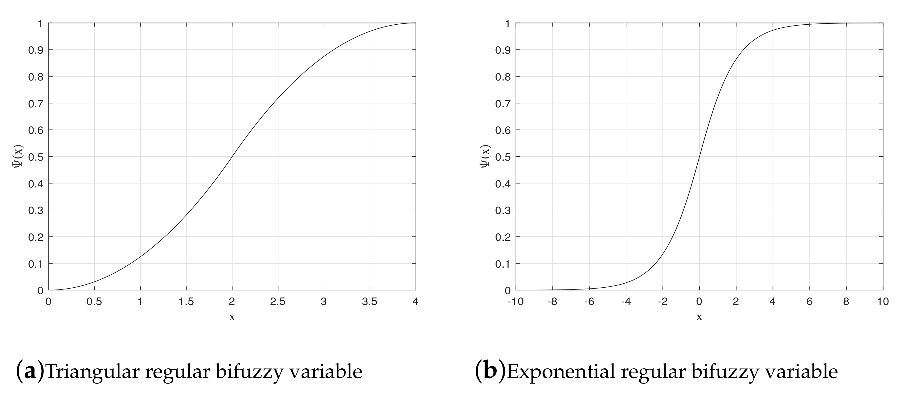
Example 9.

Assume that $\widetilde{\tilde{\mathsf{\kappa }}}$ is a triangular regular bifuzzy variable, given as $\mathcal{T}(\tilde{\mathsf{\kappa }}-1,\tilde{\mathsf{\kappa }},\tilde{\mathsf{\kappa }}+1)$ with $\tilde{\mathsf{\kappa }}=\mathcal{T}(1,2,3)$. Then, the inverse credibility distribution of $\tilde{\mathsf{\kappa }}$ can be derived as ${\mathsf{{\rm Y}}}_{\tilde{\mathsf{\kappa }}}^{-1}\left(\beta \right)=2\beta +1$ according to Equation (7). Subsequently, for any $\beta \in (0,1)$, the triplet $\mathcal{T}(2\beta ,2\beta +1,2\beta +2)$ represents a secondary fuzzy number of $\widetilde{\tilde{\mathsf{\kappa }}}$, and so using Equation (6), the measurable function $\mathrm{Cr}\{\tilde{\zeta }\le x\}$ is

$$\mathrm{Cr}\{\tilde{\zeta }\le x\}=\left\{\begin{array}{cc}{\displaystyle 0},\hfill & \mathrm{if}x\le 2\beta \hfill \\ {\displaystyle \frac{x-2\beta }{2}},\hfill & \mathrm{if}2\beta <x\le 2\beta +2\hfill \\ {\displaystyle 1},\hfill & \mathrm{if}x>2\beta +2.\hfill \end{array}\right.$$

(19)

Based on that, by Theorem 4, the triangular regular bifuzzy variable $\widetilde{\tilde{\mathsf{\kappa }}}$ has the mean chance distribution

$$\begin{array}{cc}\hfill {\mathrm{Ch}}^M\{\widetilde{\tilde{\mathsf{\kappa }}}\le x\}=& \left\{\begin{array}{cc}{\displaystyle {\int }_0^{1}0\mathrm{d}\beta },\hfill & \mathrm{if}x\le 0\hfill \\ {\displaystyle {\int }_0^{\frac{x}{2}}\frac{x-2\beta }{2}\mathrm{d}\beta },\hfill & \mathrm{if}0<x\le 2\hfill \\ {\displaystyle {\int }_0^{\frac{x-2}{2}}1\mathrm{d}\beta +{\int }_{\frac{x-2}{2}}^1\frac{x-2\beta }{2}\mathrm{d}\beta },\hfill & \mathrm{if}2<x\le 4\hfill \\ {\displaystyle {\int }_0^{1}1\mathrm{d}\beta },\hfill & \mathrm{if}x>4\hfill \end{array}\right.\hfill \\ \\ \hfill =& \left\{\begin{array}{cc}{\displaystyle 0},\hfill & \mathrm{if}x\le 0\hfill \\ {\displaystyle \frac{1}{8}{x}^2},\hfill & \mathrm{if}0<x\le 2\hfill \\ {\displaystyle x-1-\frac{1}{8}{x}^2},\hfill & \mathrm{if}2<x\le 4\hfill \\ {\displaystyle 1},\hfill & \mathrm{if}x>4,\hfill \end{array}\right.\hfill \end{array}$$

(20)

which is depicted in Figure 2a.

Example 10.

Assume that $\widetilde{\tilde{\mathsf{\kappa }}}$ is an exponential regular bifuzzy variable, given as $\mathcal{E}(\tilde{\mathsf{\kappa }},1,1)$, where $\tilde{\mathsf{\kappa }}=\mathcal{E}(0,1,1)$. According to Equation (9), the inverse credibility distribution of $\tilde{\mathsf{\kappa }}$ is

$${\mathsf{{\rm Y}}}_{\tilde{\mathsf{\kappa }}}^{-1}\left(\beta \right)=\left\{\begin{array}{cc}{\displaystyle ln\left(2\beta \right)},\hfill & \mathrm{if}0<\beta \le 0.5\hfill \\ {\displaystyle -ln(2-2\beta )},\hfill & \mathrm{if}0.5<\beta <1.\hfill \end{array}\right.$$

(21)

Subsequently, for $\beta \in (0,0.5)$, by using Equation (8), the measurable function $\mathrm{Cr}\{\tilde{\zeta }\le x\}$ is

$$\mathrm{Cr}\{\tilde{\zeta }\le x\}=\left\{\begin{array}{cc}{\displaystyle \frac{1}{2}{e}^{x-ln\left(2\beta \right)}},\hfill & \mathrm{if}x\le ln\left(2\beta \right)\hfill \\ {\displaystyle 1-\frac{1}{2}{e}^{ln\left(2\beta \right)-x}},\hfill & \mathrm{if}x>ln\left(2\beta \right),\hfill \end{array}\right.$$

(22)

and for $\beta \in (0.5,1)$,

$$\mathrm{Cr}\{\tilde{\zeta }\le x\}=\left\{\begin{array}{cc}{\displaystyle \frac{1}{2}{e}^{x+ln(2-2\beta )}},\hfill & \mathrm{if}x\le -ln(2-2\beta )\hfill \\ {\displaystyle 1-\frac{1}{2}{e}^{-ln(2-2\beta )-x}},\hfill & \mathrm{if}x>-ln(2-2\beta ).\hfill \end{array}\right.$$

(23)

Then, the computing result of the mean chance distribution of the exponential regular bifuzzy variable $\widetilde{\tilde{\mathsf{\kappa }}}$ is

$$\begin{array}{cc}\hfill {\mathrm{Ch}}^M\{\widetilde{\tilde{\mathsf{\kappa }}}\le x\}=& \left\{\begin{array}{c}{\displaystyle {\int }_0^{\frac{1}{2}{e}^x}A\mathrm{d}\beta +{\int }_{\frac{1}{2}{e}^x}^{0.5}\frac{1}{2}{e}^{x-ln\left(2\beta \right)}\mathrm{d}\beta +{\int }_{0.5}^{1}B\mathrm{d}\beta },\hfill \\ \hfill & \mathrm{if}x\le 0\hfill \\ {\displaystyle {\int }_0^{0.5}A\mathrm{d}\beta +{\int }_{0.5}^{1-\frac{1}{2}{e}^{-x}}(1-\frac{1}{2}{e}^{-ln(2-2\beta )-x})\mathrm{d}\beta +{\int }_{1-\frac{1}{2}{e}^{-x}}^{1}B\mathrm{d}\beta },\hfill \\ \hfill & \mathrm{if}x>0\hfill \end{array}\right.\hfill \\ \\ \hfill =& \left\{\begin{array}{cc}{\displaystyle \frac{e^x}{2}-\frac{x{e}^x}{4}},\hfill & \mathrm{if}x\le 0\hfill \\ {\displaystyle 1-\frac{e^{-x}}{2}-\frac{x{e}^{-x}}{4}},\hfill & \mathrm{if}x>0,\hfill \end{array}\right.\hfill \end{array}$$

(24)

where A and B represent the functions $1-\frac{1}{2}{e}^{ln\left(2\beta \right)-x}$ and $\frac{1}{2}{e}^{x+ln(2-2\beta )}$, respectively. Afterwards, this distribution is shown in Figure 2b.

3.2. Operational Law

In particular, to provide arithmetic operations for analytically and explicitly calculating the mean chance distribution of the strictly monotone and continuous function of independent regular bifuzzy variables, we first review the operational law for regular LR fuzzy numbers introduced by Zhou et al. [22], which is documented as follows.

Theorem 5.

(Zhou et al. [22]) Suppose that ${\tilde{\tau }}_i$ is a regular LR fuzzy variable with the inverse credibility distribution ${\mathsf{{\rm Y}}}_{{\tilde{\mathsf{\kappa }}}_i}^{-1}$, for $i=1,2,\cdots ,n$. If ${\tilde{\tau }}_1,{\tilde{\tau }}_2,\cdots ,{\tilde{\tau }}_n$ are independent, and the function $g(s_1,s_2,\cdots ,s_n)$ is strictly increasing with reference to $s_1,s_2,\cdots ,s_t$ and strictly decreasing with reference to $s_{t+1},s_{t+2},\cdots ,s_n$, then denote $\tilde{\mathbf{\tau }}=g({\tilde{\tau }}_1,{\tilde{\tau }}_2,\cdots ,{\tilde{\tau }}_n)$, and the inverse credibility distribution of $\tilde{\mathbf{\tau }}$ is

$${\mathsf{{\rm Y}}}_{\tilde{\mathbf{\tau }}}^{-1}\left(\beta \right)=g({\mathsf{{\rm Y}}}_{{\tilde{\tau }}_1}^{-1}\left(\beta \right),\cdots ,{\mathsf{{\rm Y}}}_{{\tilde{\tau }}_t}^{-1}\left(\beta \right),{\mathsf{{\rm Y}}}_{{\tilde{\tau }}_{t+1}}^{-1}(1-\beta ),\cdots ,{\mathsf{{\rm Y}}}_{{\tilde{\tau }}_n}^{-1}(1-\beta )).$$

(25)

Next, based on the special type function with the characteristics of strictly monotone and continuous, the useful arithmetic operations for regular bifuzzy variables on the basis of Theorem 5 will be presented in the following.

Theorem 6.

(Operational law) Suppose that ${\widetilde{\tilde{\mathsf{\kappa }}}}_i$ is a regular bifuzzy variable and the primary fuzzy number ${\tilde{\mathsf{\kappa }}}_i$ of ${\widetilde{\tilde{\mathsf{\kappa }}}}_i$ has the inverse credibility distribution ${\mathsf{{\rm Y}}}_{{\tilde{\mathsf{\kappa }}}_i}^{-1}$, for $i=1,2,\cdots ,n$. If ${\widetilde{\tilde{\mathsf{\kappa }}}}_1,{\widetilde{\tilde{\mathsf{\kappa }}}}_2,\cdots ,{\widetilde{\tilde{\mathsf{\kappa }}}}_n$ are independent, and the function $g(s_1,s_2,\cdots ,s_n)$ is strictly increasing with reference to $s_1,s_2,\cdots ,s_t$ and strictly decreasing with reference to $s_{t+1},s_{t+2},\cdots ,s_n$, then $g({\widetilde{\tilde{\mathsf{\kappa }}}}_1,{\widetilde{\tilde{\mathsf{\kappa }}}}_2,\cdots ,{\widetilde{\tilde{\mathsf{\kappa }}}}_n)$, denoted as $\widetilde{\tilde{\mathbf{\kappa }}}$, has the mean chance distribution

$${\mathrm{Ch}}^M\{g({\widetilde{\tilde{\mathsf{\kappa }}}}_1,{\widetilde{\tilde{\mathsf{\kappa }}}}_2,\cdots ,{\widetilde{\tilde{\mathsf{\kappa }}}}_n)\le x\}={\int }_0^1\mathrm{Cr}\{g({\tilde{\zeta }}_1,{\tilde{\zeta }}_2,\cdots ,{\tilde{\zeta }}_n)\le x\}\mathrm{d}\beta ,\forall x\in \mathbb{R},$$

(26)

where ${\tilde{\zeta }}_i$ is a secondary fuzzy number of ${\widetilde{\tilde{\mathsf{\kappa }}}}_i$, expressed as

$${\tilde{\zeta }}_i=\left\{\begin{array}{cc}{({\mathsf{{\rm Y}}}_{{\tilde{\mathsf{\kappa }}}_i}^{-1}\left(\beta \right),{\iota }_i,{\upsilon }_i)}_{L_i{R}_i},\hfill & i=1,2,\cdots ,t\hfill \\ {({\mathsf{{\rm Y}}}_{{\tilde{\mathsf{\kappa }}}_i}^{-1}(1-\beta ),{\iota }_i,{\upsilon }_i)}_{L_i{R}_i},\hfill & i=t+1,t+2,\cdots ,n,\hfill \end{array}\right.$$

(27)

with respect to β.

Proof of Theorem 6. 

At first, it is obvious that the primary fuzzy number of $\widetilde{\tilde{\mathbf{\kappa }}}$ can be written as $\tilde{\mathbf{\kappa }}=g({\tilde{\mathsf{\kappa }}}_1,{\tilde{\mathsf{\kappa }}}_2,\cdots ,{\tilde{\mathsf{\kappa }}}_n)$, and on account of Theorem 5, its inverse credibility distribution could be formulated by

$${\mathsf{{\rm Y}}}_{\tilde{\mathbf{\kappa }}}^{-1}\left(\beta \right)=g({\mathsf{{\rm Y}}}_{{\tilde{\mathsf{\kappa }}}_1}^{-1}\left(\beta \right),\cdots ,{\mathsf{{\rm Y}}}_{{\tilde{\mathsf{\kappa }}}_t}^{-1}\left(\beta \right),{\mathsf{{\rm Y}}}_{{\tilde{\mathsf{\kappa }}}_{t+1}}^{-1}(1-\beta ),\cdots ,{\mathsf{{\rm Y}}}_{{\tilde{\mathsf{\kappa }}}_n}^{-1}(1-\beta )).$$

Subsequently, following from Theorems 4, this theorem is naturally verified. □

Theoretically, it is not easy to obtain the measurable function, i.e., $\mathrm{Cr}\{g({\tilde{\zeta }}_1,{\tilde{\zeta }}_2,\cdots ,{\tilde{\zeta }}_n)\le x\}$, directly in Equation (26). Thus, considering the relationship between the credibility distribution and the inverse credibility distribution of a regular LR fuzzy number, we can further derive the equivalent form of the above theorem via an inverse operation.

Theorem 7.

Suppose that ${\widetilde{\tilde{\mathsf{\kappa }}}}_i$ is a regular bifuzzy variable and the primary fuzzy number ${\tilde{\mathsf{\kappa }}}_i$ of ${\widetilde{\tilde{\mathsf{\kappa }}}}_i$ has the inverse credibility distribution ${\mathsf{{\rm Y}}}_{{\tilde{\mathsf{\kappa }}}_i}^{-1}$, for $i=1,2,\cdots ,n$. If ${\widetilde{\tilde{\mathsf{\kappa }}}}_1,{\widetilde{\tilde{\mathsf{\kappa }}}}_2,\cdots ,{\widetilde{\tilde{\mathsf{\kappa }}}}_n$ are independent, and the function $g(s_1,s_2,\cdots ,s_n)$ is strictly increasing with reference to $s_1,s_2,\cdots ,s_t$ and strictly decreasing with reference to $s_{t+1},s_{t+2},\cdots ,s_n$, then for any $x\in \mathbb{R}$, we have

$${\mathrm{Ch}}^M\{g({\widetilde{\tilde{\mathsf{\kappa }}}}_1,{\widetilde{\tilde{\mathsf{\kappa }}}}_2,\cdots ,{\widetilde{\tilde{\mathsf{\kappa }}}}_n)\le x\}={\int }_0^{1}F\left(g({\tilde{\zeta }}_1,{\tilde{\zeta }}_2,\cdots ,{\tilde{\zeta }}_n)\right)\mathrm{d}\beta ,$$

(28)

where $F\left(g({\tilde{\zeta }}_1,{\tilde{\zeta }}_2,\cdots ,{\tilde{\zeta }}_n)\right)$ is the solution α of the equation that the inverse credibility distribution of $g({\tilde{\zeta }}_1,{\tilde{\zeta }}_2,\cdots ,{\tilde{\zeta }}_n)$ is equal to x, i.e.,

$$g({\mathsf{{\rm Y}}}_{{\tilde{\zeta }}_1}^{-1}\left(\alpha \right),\cdots ,{\mathsf{{\rm Y}}}_{{\tilde{\zeta }}_t}^{-1}\left(\alpha \right),{\mathsf{{\rm Y}}}_{{\tilde{\zeta }}_{t+1}}^{-1}(1-\alpha ),\cdots ,{\mathsf{{\rm Y}}}_{{\tilde{\zeta }}_n}^{-1}(1-\alpha ))=x,$$

(29)

and ${\tilde{\zeta }}_i$ is a secondary fuzzy number of ${\widetilde{\tilde{\mathsf{\kappa }}}}_i$, expressed as

$${\tilde{\zeta }}_i=\left\{\begin{array}{cc}{({\mathsf{{\rm Y}}}_{{\tilde{\mathsf{\kappa }}}_i}^{-1}\left(\beta \right),{\iota }_i,{\upsilon }_i)}_{L_i{R}_i},\hfill & i=1,2,\cdots ,t\hfill \\ {({\mathsf{{\rm Y}}}_{{\tilde{\mathsf{\kappa }}}_i}^{-1}(1-\beta ),{\iota }_i,{\upsilon }_i)}_{L_i{R}_i},\hfill & i=t+1,t+2,\cdots ,n,\hfill \end{array}\right.$$

(30)

with respect to β.

Proof of Theorem 7. 

It follows from Theorem 6 that this case is valid if and only if for any real number $\beta$, the equation $F\left(g({\tilde{\zeta }}_1,{\tilde{\zeta }}_2,\cdots ,{\tilde{\zeta }}_n)\right)=\mathrm{Cr}\{g({\tilde{\zeta }}_1,{\tilde{\zeta }}_2,\cdots ,{\tilde{\zeta }}_n)\le x\}$ holds. In fact, since the fuzzy variables ${\tilde{\zeta }}_1,{\tilde{\zeta }}_2,\cdots ,{\tilde{\zeta }}_n$ are regular LR, on account of Theorem 5, if we write $\tilde{\mathbf{\zeta }}=g({\tilde{\zeta }}_1,{\tilde{\zeta }}_2,\cdots ,{\tilde{\zeta }}_n)$, then $\tilde{\mathbf{\zeta }}$ is a regular LR fuzzy variable with the inverse credibility distribution

$${\mathsf{{\rm Y}}}_{\tilde{\mathbf{\zeta }}}^{-1}\left(\alpha \right)=g({\mathsf{{\rm Y}}}_{{\tilde{\zeta }}_1}^{-1}\left(\alpha \right),\cdots ,{\mathsf{{\rm Y}}}_{{\tilde{\zeta }}_t}^{-1}\left(\alpha \right),{\mathsf{{\rm Y}}}_{{\tilde{\zeta }}_{t+1}}^{-1}(1-\alpha ),\cdots ,{\mathsf{{\rm Y}}}_{{\tilde{\zeta }}_n}^{-1}(1-\alpha )).$$

Meanwhile, we know that the credibility distribution of $\tilde{\mathbf{\zeta }}$ can be described as ${\mathsf{{\rm Y}}}_{\tilde{\mathbf{\zeta }}}\left(x\right)=\mathrm{Cr}\{g({\tilde{\zeta }}_1,{\tilde{\zeta }}_2,\cdots ,{\tilde{\zeta }}_n)\le x\}$, and so the root value $\alpha$ obtained in Equation (29) is exactly equal to ${\mathsf{{\rm Y}}}_{\tilde{\mathbf{\zeta }}}\left(x\right)$ for any real number x. That is, this theorem is naturally verified. □

Remark 6.

Note that for any $\beta \in (0,1)$, the inverse credibility distributions of the regular LR fuzzy variables ${\tilde{\zeta }}_1,{\tilde{\zeta }}_2,\cdots ,{\tilde{\zeta }}_n$ are determined, respectively. Thus, the function $g({\mathsf{{\rm Y}}}_{{\tilde{\zeta }}_1}^{-1}\left(\alpha \right),\cdots ,{\mathsf{{\rm Y}}}_{{\tilde{\zeta }}_t}^{-1}\left(\alpha \right),{\mathsf{{\rm Y}}}_{{\tilde{\zeta }}_{t+1}}^{-1}(1-\alpha ),\cdots ,{\mathsf{{\rm Y}}}_{{\tilde{\zeta }}_n}^{-1}(1-\alpha ))$ is strictly monotone and continuous with regard to α, and so we could simulate the value of the root in Equation (29) through the golden section or bisection method.

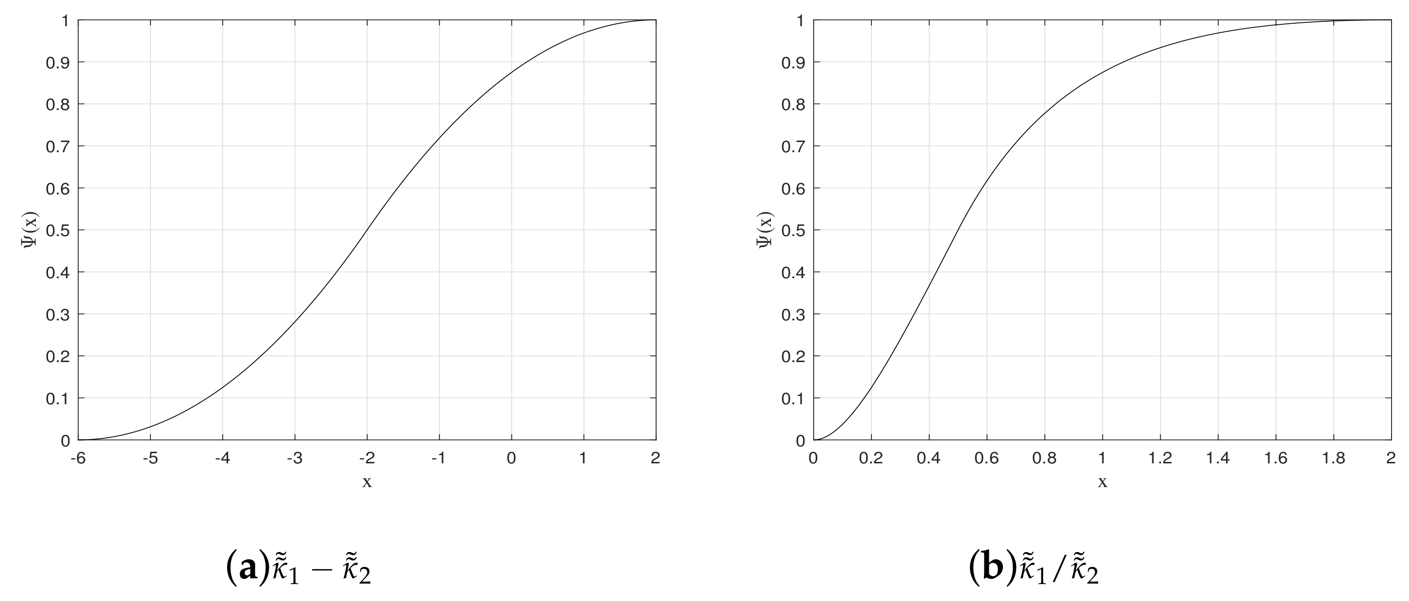
Example 11.

Assume that ${\widetilde{\tilde{\mathsf{\kappa }}}}_1$ and ${\widetilde{\tilde{\mathsf{\kappa }}}}_2$ are two triangular regular bifuzzy variables, e.g., ${\widetilde{\tilde{\mathsf{\kappa }}}}_1=\mathcal{T}({\tilde{\mathsf{\kappa }}}_1-1,{\tilde{\mathsf{\kappa }}}_1,{\tilde{\mathsf{\kappa }}}_1+1)$ with ${\tilde{\mathsf{\kappa }}}_1=\mathcal{T}(1,2,3)$ and ${\widetilde{\tilde{\mathsf{\kappa }}}}_2=\mathcal{T}({\tilde{\mathsf{\kappa }}}_2-1,{\tilde{\mathsf{\kappa }}}_2,{\tilde{\mathsf{\kappa }}}_2+1)$ with ${\tilde{\mathsf{\kappa }}}_2=\mathcal{T}(3,4,5)$. The inverse credibility distributions of the primary fuzzy numbers of ${\widetilde{\tilde{\mathsf{\kappa }}}}_1$ and ${\widetilde{\tilde{\mathsf{\kappa }}}}_2$ are described as $2\beta +1$ and $2\beta +3$, respectively. If the function $g_1(s_1,s_2)=s_1-s_2$, then we denote $\widetilde{\tilde{\mathbf{\kappa }}}=g_1({\widetilde{\tilde{\mathsf{\kappa }}}}_1,{\widetilde{\tilde{\mathsf{\kappa }}}}_2)$. For any $\beta \in (0,1)$, we have ${\tilde{\zeta }}_1=\mathcal{T}(2\beta ,2\beta +1,2\beta +2)$ and ${\tilde{\zeta }}_2=\mathcal{T}(4-2\beta ,5-2\beta ,6-2\beta )$. Consequently, the triplet $\mathcal{T}(4\beta -6,4\beta -4,4\beta -2)$ represents a secondary fuzzy number of $\widetilde{\tilde{\mathbf{\kappa }}}$ with respect to β. Then,

$$\mathrm{Cr}\{g_1({\tilde{\zeta }}_1,{\tilde{\zeta }}_2)\le x\}=\left\{\begin{array}{cc}{\displaystyle 0},\hfill & \mathrm{if}x\le 4\beta -6\hfill \\ {\displaystyle \frac{6+x-4\beta }{4}},\hfill & \mathrm{if}4\beta -6<x\le 4\beta -2\hfill \\ {\displaystyle 1},\hfill & \mathrm{if}x>4\beta -2,\hfill \end{array}\right.$$

(31)

and so by means of Theorem 6, it can be concluded that

$$\begin{array}{cc}\hfill {\mathrm{Ch}}^M\{g_1({\widetilde{\tilde{\mathsf{\kappa }}}}_1,{\widetilde{\tilde{\mathsf{\kappa }}}}_2)\le x\}=& \left\{\begin{array}{cc}{\displaystyle {\int }_0^{1}0\mathrm{d}\beta },\hfill & \mathrm{if}x\le -6\hfill \\ {\displaystyle {\int }_0^{\frac{x+6}{4}}\frac{6+x-4\beta }{4}\mathrm{d}\beta },\hfill & \mathrm{if}-6<x\le -2\hfill \\ {\displaystyle {\int }_0^{\frac{x+2}{4}}1\mathrm{d}\beta +{\int }_{\frac{x+2}{4}}^1\frac{6+x-4\beta }{4}\mathrm{d}\beta },\hfill & \mathrm{if}-2<x\le 2\hfill \\ {\displaystyle {\int }_0^{1}1\mathrm{d}\beta },\hfill & \mathrm{if}x>2\hfill \end{array}\right.\hfill \\ \\ \hfill =& \left\{\begin{array}{cc}{\displaystyle 0},\hfill & \mathrm{if}x\le -6\hfill \\ {\displaystyle \frac{{(x+6)}^2}{32}},\hfill & \mathrm{if}-6<x\le -2\hfill \\ {\displaystyle \frac{x}{4}-\frac{(x-2)(x+6)}{32}+\frac{1}{2}},\hfill & \mathrm{if}-2<x\le 2\hfill \\ {\displaystyle 1},\hfill & \mathrm{if}x>2,\hfill \end{array}\right.\hfill \end{array}$$

(32)

which is depicted in Figure 3a.

Example 12.

Assume that ${\widetilde{\tilde{\mathsf{\kappa }}}}_1$ and ${\widetilde{\tilde{\mathsf{\kappa }}}}_2$ are two triangular regular bifuzzy variables, e.g., ${\widetilde{\tilde{\mathsf{\kappa }}}}_1=\mathcal{T}({\tilde{\mathsf{\kappa }}}_1-1,{\tilde{\mathsf{\kappa }}}_1,{\tilde{\mathsf{\kappa }}}_1+1)$ with ${\tilde{\mathsf{\kappa }}}_1=\mathcal{T}(1,2,3)$ and ${\widetilde{\tilde{\mathsf{\kappa }}}}_2=\mathcal{T}({\tilde{\mathsf{\kappa }}}_2-1,{\tilde{\mathsf{\kappa }}}_2,{\tilde{\mathsf{\kappa }}}_2+1)$ with ${\tilde{\mathsf{\kappa }}}_2=\mathcal{T}(3,4,5)$. Set the function $g_2(s_1,s_2)=s_1/s_2$ and denote $\widetilde{\tilde{\mathbf{\kappa }}}=g_2({\widetilde{\tilde{\mathsf{\kappa }}}}_1,{\widetilde{\tilde{\mathsf{\kappa }}}}_2)$. Obviously, since ${\widetilde{\tilde{\mathsf{\kappa }}}}_1$ is non-negative and ${\widetilde{\tilde{\mathsf{\kappa }}}}_2$ is positive, it follows from Theorem 7 that for any $\beta \in (0,1)$, the inverse credibility distribution of $g_2({\tilde{\zeta }}_1,{\tilde{\zeta }}_2)$ can be deduced as $\frac{2\beta +2\alpha }{6-2\beta -2\alpha }$, and according to Equation (29), the root value α is equal to $\frac{3x-x\beta -\beta }{1+x}$. Thus, we have

$$\mathrm{Cr}\{g_2({\tilde{\zeta }}_1,{\tilde{\zeta }}_2)\le x\}=\left\{\begin{array}{cc}{\displaystyle 0},\hfill & {\displaystyle \mathrm{if}x\le \frac{2\beta }{6-2\beta }}\hfill \\ {\displaystyle \frac{3x-x\beta -\beta }{1+x}},\hfill & {\displaystyle \mathrm{if}\frac{2\beta }{6-2\beta }<x\le \frac{2\beta +2}{4-2\beta }}\hfill \\ {\displaystyle 1},\hfill & {\displaystyle \mathrm{if}x>\frac{2\beta +2}{4-2\beta },}\hfill \end{array}\right.$$

(33)

and so the mean chance distribution of $\widetilde{\tilde{\mathbf{\kappa }}}$ is formulated as

$$\begin{array}{cc}\hfill {\mathrm{Ch}}^M\{g_2({\widetilde{\tilde{\mathsf{\kappa }}}}_1,{\widetilde{\tilde{\mathsf{\kappa }}}}_2)\le x\}=& \left\{\begin{array}{cc}{\displaystyle {\int }_0^{1}0\mathrm{d}\beta },\hfill & \mathrm{if}x\le 0\hfill \\ {\displaystyle {\int }_0^{\frac{3x}{1+x}}\frac{3x-x\beta -\beta }{1+x}\mathrm{d}\beta },\hfill & \mathrm{if}0<x\le 0.5\hfill \\ {\displaystyle {\int }_0^{\frac{2x-1}{1+x}}1\mathrm{d}\beta +{\int }_{\frac{2x-1}{1+x}}^1\frac{3x-x\beta -\beta }{1+x}\mathrm{d}\beta },\hfill & \mathrm{if}0.5<x\le 2\hfill \\ {\displaystyle {\int }_0^{1}1\mathrm{d}\beta },\hfill & \mathrm{if}x>2\hfill \end{array}\right.\hfill \\ \\ \hfill =& \left\{\begin{array}{cc}{\displaystyle 0},\hfill & \mathrm{if}x\le 0\hfill \\ {\displaystyle \frac{9x^2}{2{(x+1)}^2}},\hfill & \mathrm{if}0<x\le 0.5\hfill \\ {\displaystyle \frac{12x+3}{2{(x+1)}^2}-\frac{3}{x+1}+\frac{1}{2}},\hfill & \mathrm{if}0.5<x\le 2\hfill \\ {\displaystyle 1},\hfill & \mathrm{if}x>2,\hfill \end{array}\right.\hfill \end{array}$$

(34)

which is depicted in Figure 3b.

Thus far, we have illustrated how to obtain the mean chance distribution via the credibility distributions and inverse credibility distributions of the primary and secondary fuzzy numbers. Apparently, this important aspect can be utilized to assist decision makers to adopt effective decisions in practical problems, e.g., the confidence level that the total cost is less than the budget.

4. Expected Value Operator

Usually, as one of the fundamental measures for uncertain events, the expected value has been given great attention by researchers, such as Dubois and Prade [24], Heilpern [25], Liu and Liu [18], etc. It should be mentioned that the first two are both defined on the basis of possibility measure, which has been proven not to satisfy the self-duality. Thus, in light of the work by Liu and Liu [18] and the self-duality of the mean chance measure demonstrated above, the expected value operator of a regular bifuzzy variable $\widetilde{\tilde{\mathsf{\kappa }}}$, defined by Choquet integrals, is given in this paper.

Theorem 8.

Suppose that $\widetilde{\tilde{\mathsf{\kappa }}}$ is a regular bifuzzy variable, and ${\mathrm{Ch}}^M$ is the mean chance measure. Then, the expected value of the variable $\widetilde{\tilde{\mathsf{\kappa }}}$, $E\left[\widetilde{\tilde{\mathsf{\kappa }}}\right]$, can be stated as

$$E\left[\widetilde{\tilde{\mathsf{\kappa }}}\right]={\int }_0^{+\infty }{\mathrm{Ch}}^M\{\widetilde{\tilde{\mathsf{\kappa }}}\ge x\}\mathrm{d}x-{\int }_{-\infty }^0{\mathrm{Ch}}^M\{\widetilde{\tilde{\mathsf{\kappa }}}\le x\}\mathrm{d}x,$$

(35)

where integrals are defined in case either of the two takes a finite value.

Proof of Theorem 8. 

Following from Definition 8 and Theorem 3, we have

$$\begin{array}{cc}\hfill E\left[\widetilde{\tilde{\mathsf{\kappa }}}\right]=& {\displaystyle {\int }_0^{+\infty }\mathrm{Cr}\left\{\theta \in \mathsf{\Theta }\left|E\right[\widetilde{\tilde{\mathsf{\kappa }}}\left(\theta \right)]\ge x\right\}\mathrm{d}x-{\int }_{-\infty }^0\mathrm{Cr}\left\{\theta \in \mathsf{\Theta }\left|E\right[\widetilde{\tilde{\mathsf{\kappa }}}\left(\theta \right)]\le x\right\}\mathrm{d}x}\hfill \\ \hfill =& {\displaystyle {\int }_{\mathsf{\Theta }}E\left[\widetilde{\tilde{\mathsf{\kappa }}}\left(\theta \right)\right]\mathrm{Cr}\left(\mathrm{d}\theta \right)}\hfill \\ \hfill =& {\displaystyle {\int }_{\mathsf{\Theta }}\left[{\int }_0^{+\infty }\mathrm{Cr}\left\{\widetilde{\tilde{\mathsf{\kappa }}}\left(\theta \right)\ge x\right\}\mathrm{d}x-{\int }_{-\infty }^0\mathrm{Cr}\left\{\widetilde{\tilde{\mathsf{\kappa }}}\left(\theta \right)\le x\right\}\mathrm{d}x\right]\mathrm{Cr}\left(\mathrm{d}\theta \right)}\hfill \\ \hfill =& {\displaystyle {\int }_0^{+\infty }{\int }_{\mathsf{\Theta }}\mathrm{Cr}\left\{\widetilde{\tilde{\mathsf{\kappa }}}\left(\theta \right)\ge x\right\}\mathrm{Cr}\left(\mathrm{d}\theta \right)\mathrm{d}x-{\int }_{-\infty }^0{\int }_{\mathsf{\Theta }}\mathrm{Cr}\left\{\widetilde{\tilde{\mathsf{\kappa }}}\left(\theta \right)\le x\right\}\mathrm{Cr}\left(\mathrm{d}\theta \right)\mathrm{d}x}\hfill \\ \hfill =& {\displaystyle {\int }_0^{+\infty }{\mathrm{Ch}}^M\{\widetilde{\tilde{\mathsf{\kappa }}}\ge x\}\mathrm{d}x-{\int }_{-\infty }^0{\mathrm{Ch}}^M\{\widetilde{\tilde{\mathsf{\kappa }}}\le x\}\mathrm{d}x.}\hfill \end{array}$$

That is, this theorem is naturally verified. □

Theorem 9.

Suppose that $\widetilde{\tilde{\mathsf{\kappa }}}$ is a regular bifuzzy variable. Then, it has the expected value

$${\displaystyle E\left[\widetilde{\tilde{\mathsf{\kappa }}}\right]={\int }_{-\infty }^{+\infty }x\mathrm{d}{\mathsf{\Psi }}_{\widetilde{\tilde{\mathsf{\kappa }}}}\left(x\right),}$$

(36)

where ${\mathsf{\Psi }}_{\widetilde{\tilde{\mathsf{\kappa }}}}$ represents the mean chance distribution of $\widetilde{\tilde{\mathsf{\kappa }}}$.

Proof of Theorem 9. 

According to Equation (15), it is known that the mean chance distribution ${\mathsf{\Psi }}_{\widetilde{\tilde{\mathsf{\kappa }}}}\left(x\right)$ is strictly increasing and continuous, and so denote ${\mathsf{\Psi }}_{\widetilde{\tilde{\mathsf{\kappa }}}}\left(x\right)={\int }_{-\infty }^x\mathrm{d}{\mathsf{\Psi }}_{\widetilde{\tilde{\mathsf{\kappa }}}}\left(y\right)$ and $1-{\mathsf{\Psi }}_{\widetilde{\tilde{\mathsf{\kappa }}}}\left(x\right)={\int }_x^{+\infty }\mathrm{d}{\mathsf{\Psi }}_{\widetilde{\tilde{\mathsf{\kappa }}}}\left(y\right)$, respectively. Following from Theorem 8, if we set ${\mathrm{Ch}}^M\{\widetilde{\tilde{\mathsf{\kappa }}}\ge x\}=1-{\mathsf{\Psi }}_{\widetilde{\tilde{\mathsf{\kappa }}}}\left(x\right)$, then an equivalent formula of Equation (35) is developed as

$$\begin{array}{cc}\hfill E\left[\widetilde{\tilde{\mathsf{\kappa }}}\right]=& {\displaystyle {\int }_0^{+\infty }(1-{\mathsf{\Psi }}_{\widetilde{\tilde{\mathsf{\kappa }}}}\left(x\right))\mathrm{d}x-{\int }_{-\infty }^0{\mathsf{\Psi }}_{\widetilde{\tilde{\mathsf{\kappa }}}}\left(x\right)\mathrm{d}x}\hfill \\ \hfill =& {\displaystyle {\int }_0^{+\infty }{\int }_x^{+\infty }\mathrm{d}{\mathsf{\Psi }}_{\widetilde{\tilde{\mathsf{\kappa }}}}\left(y\right)\mathrm{d}x-{\int }_{-\infty }^0{\int }_{-\infty }^x\mathrm{d}{\mathsf{\Psi }}_{\widetilde{\tilde{\mathsf{\kappa }}}}\left(y\right)\mathrm{d}x}\hfill \\ \hfill =& {\displaystyle {\int }_0^{+\infty }{\int }_0^y\mathrm{d}x\mathrm{d}{\mathsf{\Psi }}_{\widetilde{\tilde{\mathsf{\kappa }}}}\left(y\right)-{\int }_{-\infty }^0{\int }_y^0\mathrm{d}x\mathrm{d}{\mathsf{\Psi }}_{\widetilde{\tilde{\mathsf{\kappa }}}}\left(y\right)}\hfill \\ \hfill =& {\displaystyle {\int }_0^{+\infty }y\mathrm{d}{\mathsf{\Psi }}_{\widetilde{\tilde{\mathsf{\kappa }}}}\left(y\right)-{\int }_{-\infty }^0(-y)\mathrm{d}{\mathsf{\Psi }}_{\widetilde{\tilde{\mathsf{\kappa }}}}\left(y\right)}\hfill \\ \hfill =& {\displaystyle {\int }_{-\infty }^{+\infty }y\mathrm{d}{\mathsf{\Psi }}_{\widetilde{\tilde{\mathsf{\kappa }}}}\left(y\right),}\hfill \end{array}$$

which is the commonly used form to calculate the expected value in uncertainty theory. Thus, Equation (36) is naturally obtained. □

Theorem 10.

Suppose that $\widetilde{\tilde{\mathsf{\kappa }}}$ is a regular bifuzzy variable. If the mean chance distribution of $\widetilde{\tilde{\mathsf{\kappa }}}$ is described as ${\mathsf{\Psi }}_{\widetilde{\tilde{\mathsf{\kappa }}}}$, and its inverse function is denoted as ${\mathsf{\Psi }}_{\widetilde{\tilde{\mathsf{\kappa }}}}^{-1}$, then $\widetilde{\tilde{\mathsf{\kappa }}}$ has the expected value

$$E\left[\widetilde{\tilde{\mathsf{\kappa }}}\right]={\int }_0^1{\mathsf{\Psi }}_{\widetilde{\tilde{\mathsf{\kappa }}}}^{-1}\left(\beta \right)\mathrm{d}\beta .$$

(37)

Proof of Theorem 10. 

Following from Theorem 9, through the change of variables of the integral, set $\beta ={\mathsf{\Psi }}_{\widetilde{\tilde{\mathsf{\kappa }}}}\left(x\right)$, and so $x={\mathsf{\Psi }}_{\widetilde{\tilde{\mathsf{\kappa }}}}^{-1}\left(\beta \right)$. Then, we have

$$\begin{array}{cc}\hfill E\left[\widetilde{\tilde{\mathsf{\kappa }}}\right]=& {\displaystyle {\int }_{-\infty }^{+\infty }x\mathrm{d}{\mathsf{\Psi }}_{\widetilde{\tilde{\mathsf{\kappa }}}}\left(y\right)}\hfill \\ \hfill =& {\displaystyle {\int }_0^1{\mathsf{\Psi }}_{\widetilde{\tilde{\mathsf{\kappa }}}}^{-1}\left(\beta \right)\mathrm{d}\beta .}\hfill \end{array}$$

Thus, Equation (37) is naturally obtained. □

Thus far, two methodologies have been introduced to mathematically formulate the expected value of the regular bifuzzy variable on the foundation of its mean chance distribution. However, it seems somewhat complicated to calculate the expectation using the above methods. Alternatively, in this regard, the following equivalent analytical formulas are proposed to obtain the expected value in a straightforward manner on the basis of works by Li [26] and Zhou et al. [22].

Theorem 11.

Suppose that $\widetilde{\tilde{\mathsf{\kappa }}}$ is a regular bifuzzy variable and the primary fuzzy number $\tilde{\mathsf{\kappa }}$ of $\widetilde{\tilde{\mathsf{\kappa }}}$ has the credibility distribution ${\mathsf{{\rm Y}}}_{\tilde{\mathsf{\kappa }}}$. Then, the expected value of $\widetilde{\tilde{\mathsf{\kappa }}}$ can be calculated by

$${\displaystyle E\left[\widetilde{\tilde{\mathsf{\kappa }}}\right]={\int }_{-\infty }^{+\infty }{\int }_{-\infty }^{+\infty }x\mathrm{d}{\mathsf{{\rm Y}}}_{\tilde{\xi }}\left(x\right)\mathrm{d}{\mathsf{{\rm Y}}}_{\tilde{\mathsf{\kappa }}}\left(y\right),}$$

(38)

where $\tilde{\xi }$ is a secondary fuzzy number of $\widetilde{\tilde{\mathsf{\kappa }}}$, expressed as ${(y,\iota ,\upsilon )}_{LR}$, with respect to y, and ${\mathsf{{\rm Y}}}_{\tilde{\xi }}$ represents the credibility distribution of $\tilde{\xi }$.

Proof of Theorem 11. 

According to Theorems 2 and 3, for all $x\in \mathbb{R}$, we have ${\mathrm{Ch}}^M\{\widetilde{\tilde{\mathsf{\kappa }}}\ge x\}=1-{\int }_{-\infty }^{+\infty }\mathrm{Cr}\{\tilde{\xi }\le x\}\mathrm{d}{\mathsf{{\rm Y}}}_{\tilde{\mathsf{\kappa }}}\left(y\right)$. Then, following from Theorem 8, we have

$${\displaystyle \begin{array}{cc}\hfill E\left[\widetilde{\tilde{\mathsf{\kappa }}}\right]=& {\displaystyle {\int }_0^{+\infty }{\mathrm{Ch}}^M\{\widetilde{\tilde{\mathsf{\kappa }}}\ge x\}\mathrm{d}x-{\int }_{-\infty }^0{\mathrm{Ch}}^M\{\widetilde{\tilde{\mathsf{\kappa }}}\le x\}\mathrm{d}x}\hfill \\ \hfill =& {\displaystyle {\int }_0^{+\infty }\left[1-{\int }_{-\infty }^{+\infty }\mathrm{Cr}\{\tilde{\xi }\le x\}\mathrm{d}{\mathsf{{\rm Y}}}_{\tilde{\mathsf{\kappa }}}\left(y\right)\right]\mathrm{d}x-{\int }_{-\infty }^0{\int }_{-\infty }^{+\infty }\mathrm{Cr}\{\tilde{\xi }\le x\}\mathrm{d}{\mathsf{{\rm Y}}}_{\tilde{\mathsf{\kappa }}}\left(y\right)\mathrm{d}x}\hfill \\ \hfill =& {\displaystyle {\int }_{-\infty }^{+\infty }{\int }_0^{+\infty }\mathrm{d}x\mathrm{d}{\mathsf{{\rm Y}}}_{\tilde{\mathsf{\kappa }}}\left(y\right)-{\int }_{-\infty }^{+\infty }{\int }_0^{+\infty }\mathrm{Cr}\{\tilde{\xi }\le x\}\mathrm{d}x\mathrm{d}{\mathsf{{\rm Y}}}_{\tilde{\mathsf{\kappa }}}\left(y\right)}\hfill \\ & -{\int }_{-\infty }^{+\infty }{\int }_{-\infty }^0\mathrm{Cr}\{\tilde{\xi }\le x\}\mathrm{d}x\mathrm{d}{\mathsf{{\rm Y}}}_{\tilde{\mathsf{\kappa }}}\left(y\right)\hfill \\ \hfill =& {\int }_{-\infty }^{+\infty }\left[{\int }_0^{+\infty }\left(1-\mathrm{Cr}\{\tilde{\xi }\le x\}\right)\mathrm{d}x-{\int }_{-\infty }^0\mathrm{Cr}\{\tilde{\xi }\le x\}\mathrm{d}x\right]\mathrm{d}{\mathsf{{\rm Y}}}_{\tilde{\mathsf{\kappa }}}\left(y\right)\hfill \\ \hfill =& {\int }_{-\infty }^{+\infty }\left[{\int }_0^{+\infty }\mathrm{Cr}\{\tilde{\xi }\ge x\}\mathrm{d}x-{\int }_{-\infty }^0\mathrm{Cr}\{\tilde{\xi }\le x\}\mathrm{d}x\right]\mathrm{d}{\mathsf{{\rm Y}}}_{\tilde{\mathsf{\kappa }}}\left(y\right)\hfill \\ \hfill =& {\int }_{-\infty }^{+\infty }E\left[\tilde{\xi }\right]\mathrm{d}{\mathsf{{\rm Y}}}_{\tilde{\mathsf{\kappa }}}\left(y\right)\hfill \\ \hfill =& {\int }_{-\infty }^{+\infty }{\int }_{-\infty }^{+\infty }x\mathrm{d}{\mathsf{{\rm Y}}}_{\tilde{\xi }}\left(x\right)\mathrm{d}{\mathsf{{\rm Y}}}_{\tilde{\mathsf{\kappa }}}\left(y\right).\hfill \end{array}}$$

Thus, Equation (38) is naturally obtained. □

Theorem 12.

Suppose that $\widetilde{\tilde{\mathsf{\kappa }}}$ is a regular bifuzzy variable and the primary fuzzy number $\tilde{\mathsf{\kappa }}$ of $\widetilde{\tilde{\mathsf{\kappa }}}$ has the inverse credibility distribution ${\mathsf{{\rm Y}}}_{\tilde{\mathsf{\kappa }}}^{-1}$. Then,

$${\displaystyle E\left[\widetilde{\tilde{\mathsf{\kappa }}}\right]={\int }_0^1{\int }_0^1{\mathsf{{\rm Y}}}_{\tilde{\zeta }}^{-1}\left(\alpha \right)\mathrm{d}\alpha \mathrm{d}\beta ,}$$

(39)

where $\tilde{\zeta }$ is a secondary fuzzy number of $\widetilde{\tilde{\mathsf{\kappa }}}$, expressed as ${({\mathsf{{\rm Y}}}_{\tilde{\mathsf{\kappa }}}^{-1}\left(\beta \right),\iota ,\upsilon )}_{LR}$, with respect to β, and ${\mathsf{{\rm Y}}}_{\tilde{\zeta }}^{-1}$ represents the inverse credibility distribution of $\tilde{\zeta }$.

Proof of Theorem 12. 

Analogously, if we denote ${\mathrm{Ch}}^M\{\widetilde{\tilde{\mathsf{\kappa }}}\ge x\}=1-{\int }_0^1\mathrm{Cr}\{\tilde{\zeta }\le x\}\mathrm{d}\beta$, then we have

$$\begin{array}{cc}\hfill E\left[\widetilde{\tilde{\mathsf{\kappa }}}\right]=& {\displaystyle {\int }_0^{+\infty }{\mathrm{Ch}}^M\{\widetilde{\tilde{\mathsf{\kappa }}}\ge x\}\mathrm{d}x-{\int }_{-\infty }^0{\mathrm{Ch}}^M\{\widetilde{\tilde{\mathsf{\kappa }}}\le x\}\mathrm{d}x}\hfill \\ \hfill =& {\displaystyle {\int }_0^{+\infty }\left[1-{\int }_0^1\mathrm{Cr}\{\tilde{\zeta }\le x\}\mathrm{d}\beta \right]\mathrm{d}x-{\int }_{-\infty }^0{\int }_0^1\mathrm{Cr}\{\tilde{\zeta }\le x\}\mathrm{d}\beta \mathrm{d}x}\hfill \\ \hfill =& {\displaystyle {\int }_0^1\left[{\int }_0^{+\infty }\mathrm{Cr}\{\tilde{\zeta }\ge x\}\mathrm{d}x-{\int }_{-\infty }^0\mathrm{Cr}\{\tilde{\zeta }\le x\}\mathrm{d}x\right]\mathrm{d}\beta }\hfill \\ \hfill =& {\displaystyle {\int }_0^{1}E\left[\tilde{\zeta }\right]\mathrm{d}\beta }\hfill \\ \hfill =& {\displaystyle {\int }_0^1{\int }_0^1{\mathsf{{\rm Y}}}_{\tilde{\zeta }}^{-1}\left(\alpha \right)\mathrm{d}\alpha \mathrm{d}\beta .}\hfill \end{array}$$

Thus, Equation (39) is naturally obtained. □

By using Theorem 12, for triangular and exponential regular bifuzzy variables, we may obtain the following conclusions for their expected values. Particularly, for Theorems 9–11, the same results will be developed.

Example 13.

If $\widetilde{\tilde{\mathsf{\kappa }}}$ is a triangular regular bifuzzy variable, i.e., $\widetilde{\tilde{\mathsf{\kappa }}}=\mathcal{T}(\tilde{\mathsf{\kappa }}-{\iota }_1,\tilde{\mathsf{\kappa }},\tilde{\mathsf{\kappa }}+{\upsilon }_1)$ with $\tilde{\mathsf{\kappa }}=\mathcal{T}(m-{\iota }_2,m,m+{\upsilon }_2)$, then the expectation of $\widetilde{\tilde{\mathsf{\kappa }}}$, $E\left[\widetilde{\tilde{\mathsf{\kappa }}}\right]$, can be deduced as

$$\begin{array}{cc}\hfill E\left[\widetilde{\tilde{\mathsf{\kappa }}}\right]=& {\displaystyle {\int }_0^1{\int }_0^1{\mathsf{{\rm Y}}}_{\tilde{\zeta }}^{-1}\left(\alpha \right)\mathrm{d}\alpha \mathrm{d}\beta }\hfill \\ \hfill =& {\displaystyle {\int }_0^{0.5}{\int }_0^{0.5}(m+{\iota }_2(2\beta -1)+{\iota }_1(2\alpha -1))\mathrm{d}\alpha \mathrm{d}\beta }\hfill \\ \hfill & {\displaystyle +{\int }_0^{0.5}{\int }_{0.5}^1(m+{\iota }_2(2\beta -1)-{\upsilon }_1(1-2\alpha ))\mathrm{d}\alpha \mathrm{d}\beta }\hfill \\ \hfill & {\displaystyle +{\int }_{0.5}^1{\int }_0^{0.5}(m-{\upsilon }_2(1-2\beta )+{\iota }_1(2\alpha -1))\mathrm{d}\alpha \mathrm{d}\beta }\hfill \\ \hfill & {\displaystyle +{\int }_{0.5}^1{\int }_{0.5}^1(m-{\upsilon }_2(1-2\beta )-{\upsilon }_1(1-2\alpha ))\mathrm{d}\alpha \mathrm{d}\beta }\hfill \\ \hfill =& {\displaystyle \frac{2m-{\iota }_1-{\iota }_2}{8}+\frac{2m+{\upsilon }_1-{\iota }_2}{8}+\frac{2m-{\iota }_1+{\upsilon }_2}{8}+\frac{2m+{\upsilon }_1+{\upsilon }_2}{8}}\hfill \\ \hfill =& {\displaystyle \frac{4m-{\iota }_1+{\upsilon }_1-{\iota }_2+{\upsilon }_2}{4},}\hfill \end{array}$$

(40)

and for Example 9, $E\left[\widetilde{\tilde{\mathsf{\kappa }}}\right]=2$.

Example 14.

If $\widetilde{\tilde{\mathsf{\kappa }}}$ is an exponential regular bifuzzy variable, i.e., $\widetilde{\tilde{\mathsf{\kappa }}}=\mathcal{E}(\tilde{\mathsf{\kappa }},p_1,p_1)$ with $\tilde{\mathsf{\kappa }}=\mathcal{E}(m,p_2,p_2)$, then its expected value is

$$\begin{array}{cc}\hfill E\left[\widetilde{\tilde{\mathsf{\kappa }}}\right]=& {\displaystyle {\int }_0^1{\int }_0^1{\mathsf{{\rm Y}}}_{\tilde{\zeta }}^{-1}\left(\alpha \right)\mathrm{d}\alpha \mathrm{d}\beta }\hfill \\ \hfill =& {\displaystyle {\int }_0^{0.5}{\int }_0^{0.5}(m+p_{2}ln\left(2\beta \right)+p_{1}ln\left(2\alpha \right))\mathrm{d}\alpha \mathrm{d}\beta }\hfill \\ \hfill & {\displaystyle +{\int }_0^{0.5}{\int }_{0.5}^1(m+p_{2}ln\left(2\beta \right)-{\upsilon }_{1}ln(2-2\alpha ))\mathrm{d}\alpha \mathrm{d}\beta }\hfill \\ \hfill & {\displaystyle +{\int }_{0.5}^1{\int }_0^{0.5}(m-{\upsilon }_{2}ln(2-2\beta )+p_{1}ln\left(2\alpha \right))\mathrm{d}\alpha \mathrm{d}\beta }\hfill \\ \hfill & {\displaystyle +{\int }_{0.5}^1{\int }_{0.5}^1(m-p_{2}ln(2-2\beta )-p_{1}ln(2-2\alpha ))\mathrm{d}\alpha \mathrm{d}\beta }\hfill \\ \hfill =& {\displaystyle \frac{m-p_1-p_2}{4}+\frac{m+p_1-p_2}{4}+\frac{m-p_1+p_2}{4}+\frac{m+p_1+p_2}{4}}\hfill \\ \hfill =& {\displaystyle m,}\hfill \end{array}$$

(41)

and for Example 10, $E\left[\widetilde{\tilde{\mathsf{\kappa }}}\right]=0$.

Not surprisingly, the expected value of a strictly monotone function with regular bifuzzy variables can be deduced via its mean chance distribution. Furthermore, based on the operational law for regular LR fuzzy variables, a novel formula is constructed for computing the expected value. Consequently, we could explicitly obtain the expectation without having to calculate the mean chance distribution.

Theorem 13.

Suppose that ${\widetilde{\tilde{\mathsf{\kappa }}}}_i$ is a regular bifuzzy variable and the primary fuzzy number ${\tilde{\mathsf{\kappa }}}_i$ of ${\widetilde{\tilde{\mathsf{\kappa }}}}_i$ has the inverse credibility distribution ${\mathsf{{\rm Y}}}_{{\tilde{\mathsf{\kappa }}}_i}^{-1}$, for $i=1,2,\cdots ,n$. If ${\widetilde{\tilde{\mathsf{\kappa }}}}_1,{\widetilde{\tilde{\mathsf{\kappa }}}}_2,\cdots ,{\widetilde{\tilde{\mathsf{\kappa }}}}_n$ are independent, and the function $g(s_1,s_2,\cdots ,s_n)$ is strictly increasing with reference to $s_1,s_2,\cdots ,s_t$ and strictly decreasing with reference to $s_{t+1},s_{t+2},\cdots ,s_n$, then denote $\widetilde{\tilde{\mathbf{\kappa }}}=g({\widetilde{\tilde{\mathsf{\kappa }}}}_1,{\widetilde{\tilde{\mathsf{\kappa }}}}_2,\cdots ,{\widetilde{\tilde{\mathsf{\kappa }}}}_n)$ and the expected value of $\widetilde{\tilde{\mathbf{\kappa }}}$ is written as

$$E\left[\widetilde{\tilde{\mathbf{\kappa }}}\right]={\int }_0^1{\int }_0^{1}g({\mathsf{{\rm Y}}}_{{\tilde{\zeta }}_1}^{-1}\left(\alpha \right),\cdots ,{\mathsf{{\rm Y}}}_{{\tilde{\zeta }}_t}^{-1}\left(\alpha \right),{\mathsf{{\rm Y}}}_{{\tilde{\zeta }}_{t+1}}^{-1}(1-\alpha ),\cdots ,{\mathsf{{\rm Y}}}_{{\tilde{\zeta }}_n}^{-1}(1-\alpha ))\mathrm{d}\alpha \mathrm{d}\beta ,$$

(42)

where ${\tilde{\zeta }}_i$ is a secondary fuzzy number of ${\widetilde{\tilde{\mathsf{\kappa }}}}_i$, expressed as

$${\tilde{\zeta }}_i=\left\{\begin{array}{cc}{({\mathsf{{\rm Y}}}_{{\tilde{\mathsf{\kappa }}}_i}^{-1}\left(\beta \right),{\iota }_i,{\upsilon }_i)}_{L_i{R}_i},\hfill & i=1,2,\cdots ,t\hfill \\ {({\mathsf{{\rm Y}}}_{{\tilde{\mathsf{\kappa }}}_i}^{-1}(1-\beta ),{\iota }_i,{\upsilon }_i)}_{L_i{R}_i},\hfill & i=t+1,t+2,\cdots ,n,\hfill \end{array}\right.$$

(43)

with respect to β.

Proof of Theorem 13. 

According to Equations (16) and (26), we set ${\mathrm{Ch}}^M\{g({\widetilde{\tilde{\mathsf{\kappa }}}}_1,{\widetilde{\tilde{\mathsf{\kappa }}}}_2,\cdots ,{\widetilde{\tilde{\mathsf{\kappa }}}}_n)\ge x\}=1-{\int }_0^1\mathrm{Cr}\{g({\tilde{\zeta }}_1,{\tilde{\zeta }}_2,\cdots ,{\tilde{\zeta }}_n)\le x\}\mathrm{d}\beta$. Then, following from Theorem 8, a similar process adopted in Theorems 11 and 12 may prove this case.

$$\begin{array}{cc}\hfill E\left[\widetilde{\tilde{\mathbf{\kappa }}}\right]=& {\displaystyle {\int }_0^{+\infty }{\mathrm{Ch}}^M\{g({\widetilde{\tilde{\mathsf{\kappa }}}}_1,{\widetilde{\tilde{\mathsf{\kappa }}}}_2,\cdots ,{\widetilde{\tilde{\mathsf{\kappa }}}}_n)\ge x\}\mathrm{d}x-{\int }_{-\infty }^0{\mathrm{Ch}}^M\{g({\widetilde{\tilde{\mathsf{\kappa }}}}_1,{\widetilde{\tilde{\mathsf{\kappa }}}}_2,\cdots ,{\widetilde{\tilde{\mathsf{\kappa }}}}_n)\le x\}\mathrm{d}x}\hfill \\ \hfill =& {\displaystyle {\int }_0^{+\infty }\left[1-{\int }_0^1\mathrm{Cr}\{g({\tilde{\zeta }}_1,{\tilde{\zeta }}_2,\cdots ,{\tilde{\zeta }}_n)\le x\}\mathrm{d}\beta \right]\mathrm{d}x}\hfill \\ & {\displaystyle -{\int }_{-\infty }^0{\int }_0^1\mathrm{Cr}\{g({\tilde{\zeta }}_1,{\tilde{\zeta }}_2,\cdots ,{\tilde{\zeta }}_n)\le x\}\mathrm{d}\beta \mathrm{d}x}\hfill \\ \hfill =& {\displaystyle {\int }_0^1\left[{\int }_0^{+\infty }\mathrm{Cr}\{g({\tilde{\zeta }}_1,{\tilde{\zeta }}_2,\cdots ,{\tilde{\zeta }}_n)\ge x\}\mathrm{d}x-{\int }_{-\infty }^0\mathrm{Cr}\{g({\tilde{\zeta }}_1,{\tilde{\zeta }}_2,\cdots ,{\tilde{\zeta }}_n)\le x\}\mathrm{d}x\right]\mathrm{d}\beta }\hfill \\ \hfill =& {\displaystyle {\int }_0^{1}E\left[g({\tilde{\zeta }}_1,{\tilde{\zeta }}_2,\cdots ,{\tilde{\zeta }}_n)\right]\mathrm{d}\beta }\hfill \\ \hfill =& {\displaystyle {\int }_0^1{\int }_0^{1}f({\mathsf{{\rm Y}}}_{{\tilde{\zeta }}_1}^{-1}\left(\alpha \right),\cdots ,{\mathsf{{\rm Y}}}_{{\tilde{\zeta }}_t}^{-1}\left(\alpha \right),{\mathsf{{\rm Y}}}_{{\tilde{\zeta }}_{t+1}}^{-1}(1-\alpha ),\cdots ,{\mathsf{{\rm Y}}}_{{\tilde{\zeta }}_n}^{-1}(1-\alpha ))\mathrm{d}\alpha \mathrm{d}\beta .}\hfill \end{array}$$

Thus, Equation (42) is naturally obtained. □

Remark 7.

Suppose that ${\widetilde{\tilde{\mathsf{\kappa }}}}_1,{\widetilde{\tilde{\mathsf{\kappa }}}}_2,\cdots ,{\widetilde{\tilde{\mathsf{\kappa }}}}_n$ are independent regular bifuzzy variables. Then,

(i) 

according to the strictly monotone definition of the function, if $g(s_1,s_2,\cdots ,s_n)$ is strictly increasing with reference to $s_1,s_2,\cdots ,s_n$, we have

$${\displaystyle E\left[g({\widetilde{\tilde{\mathsf{\kappa }}}}_1,{\widetilde{\tilde{\mathsf{\kappa }}}}_2,\cdots ,{\widetilde{\tilde{\mathsf{\kappa }}}}_n)\right]={\int }_0^1{\int }_0^{1}f({\mathsf{{\rm Y}}}_{{\tilde{\zeta }}_1}^{-1}\left(\alpha \right),{\mathsf{{\rm Y}}}_{{\tilde{\zeta }}_2}^{-1}\left(\alpha \right),\cdots ,{\mathsf{{\rm Y}}}_{{\tilde{\zeta }}_n}^{-1}\left(\alpha \right))\mathrm{d}\alpha \mathrm{d}\beta ,}$$

(44)

where ${\tilde{\zeta }}_i$ is a secondary fuzzy number of ${\widetilde{\tilde{\mathsf{\kappa }}}}_i$, expressed as ${({\mathsf{{\rm Y}}}_{{\tilde{\mathsf{\kappa }}}_i}^{-1}\left(\beta \right),{\iota }_i,{\upsilon }_i)}_{L_i{R}_i}$, with respect to β, for $i=1,2,\cdots ,n$;

(ii) 

if $g(s_1,s_2,\cdots ,s_n)$ is strictly decreasing with reference to $s_1,s_2,\cdots ,s_n$, we have

$${\displaystyle E\left[g({\widetilde{\tilde{\mathsf{\kappa }}}}_1,{\widetilde{\tilde{\mathsf{\kappa }}}}_2,\cdots ,{\widetilde{\tilde{\mathsf{\kappa }}}}_n)\right]={\int }_0^1{\int }_0^{1}f({\mathsf{{\rm Y}}}_{{\tilde{\zeta }}_1}^{-1}(1-\alpha ),{\mathsf{{\rm Y}}}_{{\tilde{\zeta }}_2}^{-1}(1-\alpha ),\cdots ,{\mathsf{{\rm Y}}}_{{\tilde{\zeta }}_n}^{-1}(1-\alpha ))\mathrm{d}\alpha \mathrm{d}\beta ,}$$

(45)

where ${\tilde{\zeta }}_i$ is a secondary fuzzy number of ${\widetilde{\tilde{\mathsf{\kappa }}}}_i$, expressed as ${({\mathsf{{\rm Y}}}_{{\tilde{\mathsf{\kappa }}}_i}^{-1}(1-\beta ),{\iota }_i,{\upsilon }_i)}_{L_i{R}_i}$, with respect to β, for $i=1,2,\cdots ,n$.

Example 15.

Assume that ${\widetilde{\tilde{\mathsf{\kappa }}}}_1$ and ${\widetilde{\tilde{\mathsf{\kappa }}}}_2$ are two independent regular bifuzzy variables, and the inverse credibility distributions of their primary fuzzy numbers are described as ${\mathsf{{\rm Y}}}_{{\tilde{\mathsf{\kappa }}}_1}^{-1}$ and ${\mathsf{{\rm Y}}}_{{\tilde{\mathsf{\kappa }}}_2}^{-1}$, respectively. If we denote the function $g_1(x_1,x_2)=x_1-x_2$, following from Theorem 13, the expected value of $g_1({\widetilde{\tilde{\mathsf{\kappa }}}}_1,{\widetilde{\tilde{\mathsf{\kappa }}}}_2)$ is

$${\displaystyle E\left[g_1({\widetilde{\tilde{\mathsf{\kappa }}}}_1,{\widetilde{\tilde{\mathsf{\kappa }}}}_2)\right]={\int }_0^1{\int }_0^1({\mathsf{{\rm Y}}}_{{\tilde{\zeta }}_1}^{-1}\left(\alpha \right)-{\mathsf{{\rm Y}}}_{{\tilde{\zeta }}_2}^{-1}(1-\alpha ))\mathrm{d}\alpha \mathrm{d}\beta .}$$

(46)

For Example 11, we have ${\tilde{\zeta }}_1=\mathcal{T}(2\beta ,2\beta +1,2\beta +2)$ and ${\tilde{\zeta }}_2=\mathcal{T}(4-2\beta ,5-2\beta ,6-2\beta )$ with respect to β. Therefore, the equations ${\mathsf{{\rm Y}}}_{{\tilde{\zeta }}_1}^{-1}\left(\alpha \right)=2\beta +2\alpha$ and ${\mathsf{{\rm Y}}}_{{\tilde{\zeta }}_2}^{-1}(1-\alpha )=6-2\beta -2\alpha$ can be derived via Equation (7), respectively. Then, the expected value of $g_1({\widetilde{\tilde{\mathsf{\kappa }}}}_1,{\widetilde{\tilde{\mathsf{\kappa }}}}_2)$ is formulated as

$${\displaystyle E\left[g_1({\widetilde{\tilde{\mathsf{\kappa }}}}_1,{\widetilde{\tilde{\mathsf{\kappa }}}}_2)\right]={\int }_0^1{\int }_0^1((2\beta +2\alpha )-(6-2\beta -2\alpha ))\mathrm{d}\alpha \mathrm{d}\beta =2.}$$

(47)

Example 16.

Assume that ${\widetilde{\tilde{\mathsf{\kappa }}}}_1$ and ${\widetilde{\tilde{\mathsf{\kappa }}}}_2$ are two independent regular bifuzzy variables, and the inverse credibility distributions of their primary fuzzy numbers are described as ${\mathsf{{\rm Y}}}_{{\tilde{\mathsf{\kappa }}}_1}^{-1}$ and ${\mathsf{{\rm Y}}}_{{\tilde{\mathsf{\kappa }}}_2}^{-1}$, respectively. Denote the function $g_2(x_1,x_2)=x_1/x_2$. For $x_1\ge 0$ and $x_2>0$, $g_2(x_1,x_2)$ is strictly increasing with regard to $x_1$ and strictly decreasing with regard to $x_2$. Therefore, if ${\widetilde{\tilde{\mathsf{\kappa }}}}_1$ is non-negative and ${\widetilde{\tilde{\mathsf{\kappa }}}}_2$ is positive, then $g_2({\widetilde{\tilde{\mathsf{\kappa }}}}_1,{\widetilde{\tilde{\mathsf{\kappa }}}}_2)$ has the expected value

$${\displaystyle E\left[g_2({\widetilde{\tilde{\mathsf{\kappa }}}}_1,{\widetilde{\tilde{\mathsf{\kappa }}}}_2)\right]={\int }_0^1{\int }_0^1\frac{{\mathsf{{\rm Y}}}_{{\tilde{\zeta }}_1}^{-1}\left(\alpha \right)}{{\mathsf{{\rm Y}}}_{{\tilde{\zeta }}_2}^{-1}(1-\alpha )}\mathrm{d}\alpha \mathrm{d}\beta .}$$

(48)

Accordingly, for Example 12, it is obvious that

$${\displaystyle E\left[g_2({\widetilde{\tilde{\mathsf{\kappa }}}}_1,{\widetilde{\tilde{\mathsf{\kappa }}}}_2)\right]={\int }_0^1{\int }_0^1\frac{2\beta +2\alpha }{6-2\beta -2\alpha }\mathrm{d}\alpha \mathrm{d}\beta =9ln3-12ln2-1.}$$

(49)

Furthermore, the linearity of the expected value operator of independent bifuzzy variables defined in Liu [6] can be mathematically proved.

Theorem 14.

Suppose that ${\widetilde{\tilde{\mathsf{\kappa }}}}_1$ and ${\widetilde{\tilde{\mathsf{\kappa }}}}_2$ are two independent regular bifuzzy variables. If $E\left[{\widetilde{\tilde{\mathsf{\kappa }}}}_1\right]$ and $E\left[{\widetilde{\tilde{\mathsf{\kappa }}}}_2\right]$, the expected values of ${\widetilde{\tilde{\mathsf{\kappa }}}}_1$ and ${\widetilde{\tilde{\mathsf{\kappa }}}}_2$, are finite, then for any two real numbers m and n, we have

$$E[m{\widetilde{\tilde{\mathsf{\kappa }}}}_1+n{\widetilde{\tilde{\mathsf{\kappa }}}}_2]=mE\left[{\widetilde{\tilde{\mathsf{\kappa }}}}_1\right]+nE\left[{\widetilde{\tilde{\mathsf{\kappa }}}}_2\right].$$

(50)

Proof of Theorem 14. 

We only prove the case $m\ge 0$ and $n\le 0$. According to Definition 10, the function $m{\widetilde{\tilde{\mathsf{\kappa }}}}_1+n{\widetilde{\tilde{\mathsf{\kappa }}}}_2$ is clearly strictly increasing with regard to ${\widetilde{\tilde{\mathsf{\kappa }}}}_1$ and strictly decreasing with regard to ${\widetilde{\tilde{\mathsf{\kappa }}}}_2$. Following from Theorem 13, we have

$$\begin{array}{cc}\hfill E[m{\widetilde{\tilde{\mathsf{\kappa }}}}_1+n{\widetilde{\tilde{\mathsf{\kappa }}}}_2]=& {\displaystyle {\int }_0^1{\int }_0^1\left[m{\mathsf{{\rm Y}}}_{{\tilde{\zeta }}_1}^{-1}\left(\alpha \right)+n{\mathsf{{\rm Y}}}_{{\tilde{\zeta }}_2}^{-1}(1-\alpha )\right]\mathrm{d}\alpha \mathrm{d}\beta }\hfill \\ \hfill =& {\displaystyle m{\int }_0^1{\int }_0^1{\mathsf{{\rm Y}}}_{{\tilde{\zeta }}_1}^{-1}\left(\alpha \right)\mathrm{d}\alpha \mathrm{d}\beta +n{\int }_0^1{\int }_0^1{\mathsf{{\rm Y}}}_{{\tilde{\zeta }}_2}^{-1}(1-\alpha )\mathrm{d}\alpha \mathrm{d}\beta .}\hfill \end{array}$$

Using the substitutions in multiple integrals, the equation

$${\int }_0^1{\int }_0^1{\mathsf{{\rm Y}}}_{{\tilde{\zeta }}_2}^{-1}(1-\alpha )\mathrm{d}\alpha \mathrm{d}\beta ={\int }_0^1{\int }_0^1{\mathsf{{\rm Y}}}_{{\widehat{\tilde{\zeta }}}_2}^{-1}\left(\alpha \right)\mathrm{d}\alpha \mathrm{d}\beta ,$$

where ${\tilde{\zeta }}_2={({\mathsf{{\rm Y}}}_{{\tilde{\mathsf{\kappa }}}_2}^{-1}(1-\beta ),{\iota }_2,{\upsilon }_2)}_{LR}$ and ${\widehat{\tilde{\zeta }}}_2={({\mathsf{{\rm Y}}}_{{\tilde{\mathsf{\kappa }}}_2}^{-1}\left(\beta \right),{\iota }_2,{\upsilon }_2)}_{LR}$, holds. Seeing Theorem 12, that is exactly the expected value of ${\widetilde{\tilde{\mathsf{\kappa }}}}_2$. Therefore, we have

$$E[m{\widetilde{\tilde{\mathsf{\kappa }}}}_1+n{\widetilde{\tilde{\mathsf{\kappa }}}}_2]=mE\left[{\widetilde{\tilde{\mathsf{\kappa }}}}_1\right]+nE\left[{\widetilde{\tilde{\mathsf{\kappa }}}}_2\right],$$

and similar proof procedures can be utilized to verify the other situations, i.e., $m\ge 0$ and $n\ge 0$, $m\le 0$ and $n\ge 0$, and $m\le 0$ and $n\le 0$. Then, this theorem is naturally verified. □

5. Conclusions

In this paper, we restricted our attention on the special case of bifuzzy variables, namely regular bifuzzy variables, especially the most frequently used types, e.g., triangular and exponential regular bifuzzy variables. Two kinds of important measures were investigated in-depth, mean chance and expected value. The major contributions of this research include the following aspects: (1) the notion of mean chance measure of regular bifuzzy variables was presented, and some properties were provided; (2) the operational law for regular bifuzzy variables was proposed, and on this foundation, the mean chance distribution of strictly monotone functions of this type of variable was developed; (3) an equivalent form of the expected value operator was constructed, and some theorems for computing the expected value of regular bifuzzy variables, as well as their strictly monotone functions, were also deduced.

Moreover, we believe that the proposed arithmetic operations and operational law are of great importance for optimization and decision making in the bifuzzy environment. In uncertain fields, dependent-chance programming, chance-constrained programming, and the expected value model are three frequently utilized approaches in handling practical problems, such as the vehicle routing problem, joint replenishment problem, and hub location problem, etc. Our proposed arithmetic operations enable the implementation of these programmings with strictly monotone functions and regular bifuzzy variables and provide a sound theoretical foundation for modeling bifuzzy phenomena, which is also one of the critical future directions of this research.

References

- Zadeh, L.A. Fuzzy sets. Inf. Control 1965, 8, 338–353. [Google Scholar] [CrossRef] [Green Version]
- Zadeh, L.A. The concept of a linguistic variable and its application to approximate reasoning—I. Inf. Sci. 1975, 8, 199–251. [Google Scholar] [CrossRef]
- Dubois, D.; Prade, H. Twofold fuzzy sets: An approach to the representation of sets with fuzzy boundaries based on possibility and necessity measures. J. Fuzzy Math. 1983, 3, 53–76. [Google Scholar]
- Atanassov, K. Intuitionistic fuzzy sets. Fuzzy Sets Syst. 1986, 20, 87–96. [Google Scholar] [CrossRef]
- Liu, B. Toward fuzzy optimization without mathematical ambiguity. Fuzzy Optim. Decis. Mak. 2002, 1, 43–63. [Google Scholar] [CrossRef]
- Liu, B. Uncertainty Theory: An Introduction to Its Axiomatic Foundations; Springer: Berlin, Germany, 2004. [Google Scholar]
- Zhou, J.; Liu, B. Analysis and algorithms of bifuzzy systems. Int. J. Uncertain. Fuzziness Knowl. Based Syst. 2004, 12, 357–376. [Google Scholar] [CrossRef] [Green Version]
- Qin, Z.F.; Li, X. The sufficient and necessary condition for chance distribution of bifuzzy variable. Soft Comput. 2011, 15, 595–599. [Google Scholar] [CrossRef]
- Xu, J.P.; Yan, F. A multi-objective decision making model for the vendor selection problem in a bifuzzy environment. Expert Syst. Appl. 2011, 38, 9684–9695. [Google Scholar] [CrossRef]
- Chakraborty, D.; Jana, D.K.; Roy, T.K. Multi-item integrated supply chain model for deteriorating items with stock dependent demand under fuzzy random and bifuzzy environments. Comput. Ind. Eng. 2015, 88, 166–180. [Google Scholar] [CrossRef]
- Bera, A.K.; Jana, D.K. Multi-item imperfect production inventory model in Bi-fuzzy environments. OPSEARCH 2017, 54, 260–282. [Google Scholar] [CrossRef]
- Deng, W.L.; Qiu, D.W. Bifuzzy discrete event systems and their supervisory control theory. IEEE Trans. Fuzzy Syst. 2015, 23, 2107–2121. [Google Scholar] [CrossRef] [Green Version]
- Deng, W.L.; Qiu, D.W. State-based decentralized diagnosis of bi-fuzzy discrete event systems. IEEE Trans. Fuzzy Syst. 2017, 25, 854–867. [Google Scholar] [CrossRef]
- Taib, C.M.I.C.; Yusoff, B.; Abdullah, M.L.; Wahab, A.F. Conflicting bifuzzy multi-attribute group decision making model with application to flood control project. Group Decis. Negot. 2016, 25, 157–180. [Google Scholar] [CrossRef]
- Shi, J.X.; Zhang, W.Y.; Zhang, S.; Chen, J. A new bifuzzy optimization method for remanufacturing scheduling using extended discrete particle swarm optimization algorithm. Comput. Ind. Eng. 2021, 156, 107219. [Google Scholar] [CrossRef]
- Liu, B. Uncertainty Theory, 2nd ed.; Springer: Heidelberg, Germany, 2007. [Google Scholar]
- Zadeh, L.A. Fuzzy sets as a basis for a theory of possibility. Fuzzy Sets Syst. 1978, 1, 3–28. [Google Scholar] [CrossRef]
- Liu, B.; Liu, Y.K. Expected value of fuzzy variable and fuzzy expected value models. IEEE Trans. Fuzzy Syst. 2002, 10, 445–450. [Google Scholar]
- Liu, B. Theory and Practice of Uncertain Programming; Physica-Verlag: Heidelberg, Germany, 2002. [Google Scholar]
- Dubois, D.; Prade, H. Operations on fuzzy numbers. Int. J. Syst. Sci. 1978, 9, 613–626. [Google Scholar] [CrossRef]
- Dubois, D.; Prade, H. Fuzzy Sets and Systems: Theory and Applications; Academic Press: New York, NY, USA, 1980. [Google Scholar]
- Zhou, J.; Yang, F.; Wang, K. Fuzzy arithmetic on LR fuzzy numbers with applications to fuzzy programming. J. Intell. Fuzzy Syst. 2016, 30, 71–87. [Google Scholar] [CrossRef]
- Liu, Y.; Liu, B. On minimum-risk problems in fuzzy random decision systems. Comput. Oper. Res. 2005, 32, 257–283. [Google Scholar] [CrossRef]
- Dubois, D.; Prade, H. The mean value of a fuzzy number. Fuzzy Sets Syst. 1987, 24, 279–300. [Google Scholar] [CrossRef]
- Heilpern, S. The expected value of a fuzzy number. Fuzzy Sets Syst. 1992, 47, 81–86. [Google Scholar] [CrossRef]
- Li, X. A numerical-integration-based simulation algorithm for expected values of strictly monotone functions of ordinary fuzzy variables. IEEE Trans. Fuzzy Syst. 2015, 23, 964–972. [Google Scholar] [CrossRef]
Figure 1.
The function curve of the bifuzzy variable in Example 6.
Figure 2.
The mean chance distributions of in Examples 9 and 10.
Figure 3.
The mean chance distributions of in Examples 11 and 12.
Publisher’s Note: MDPI stays neutral with regard to jurisdictional claims in published maps and institutional affiliations. |
© 2021 by the authors. Licensee MDPI, Basel, Switzerland. This article is an open access article distributed under the terms and conditions of the Creative Commons Attribution (CC BY) license (https://creativecommons.org/licenses/by/4.0/).
Share and Cite
MDPI and ACS Style
Wang, G.; Shen, Y.; Jiang, Y.; Chen, J. The Scalar Mean Chance and Expected Value of Regular Bifuzzy Variables. Symmetry 2021, 13, 1428. https://0-doi-org.brum.beds.ac.uk/10.3390/sym13081428
AMA Style
Wang G, Shen Y, Jiang Y, Chen J. The Scalar Mean Chance and Expected Value of Regular Bifuzzy Variables. Symmetry. 2021; 13(8):1428. https://0-doi-org.brum.beds.ac.uk/10.3390/sym13081428
Chicago/Turabian StyleWang, Guang, Yixuan Shen, Yujiao Jiang, and Jiahao Chen. 2021. "The Scalar Mean Chance and Expected Value of Regular Bifuzzy Variables" Symmetry 13, no. 8: 1428. https://0-doi-org.brum.beds.ac.uk/10.3390/sym13081428
Note that from the first issue of 2016, this journal uses article numbers instead of page numbers. See further details here.