Interval Observers for Discrete-Time Linear Systems with Uncertainties

Abstract

In this paper, we consider the problem involved when designing the interval observer for the system described by a linear discrete-time model under external disturbances and measurement noises. To solve this problem, we used the reduced order model of the initial system, which is insensitive or has minimal sensitivity to the disturbances. The relations involved in designing the interval observer, which has minimal dimensions and estimates the prescribed linear function of the original system state vector, were obtained. The theoretical results were illustrated by a practical example.

1. Introduction

The problem of estimating the system state vector is critical in many practical applications. The main problems involved in designing an estimator are the system complexity and different uncertainties (external disturbances, measurement noises, and unknown parameters). Sliding mode observers can solve this problem [1,2,3] in some cases; however, under uncertainties, the estimation error is never equal to zero. This problem has recently been solved based on interval observers, which are used to evaluate the dynamic system state. One advantage of interval observers is that they can take into account many types of uncertainties in the system under consideration.

Different kinds of observers have been developed for many types of models: for continuous-time linear and non-linear [4,5,6,7,8,9,10,11], discrete-time [12,13], time delay [14,15], switched system [16,17], and singular [14]; the stability of interval observers was studied in [18]. Moreover, they have been successfully applied to solve many practical problems [19,20,21]. Exhaustive reviews are in [15,22,23].

It should be noted that all of the above-mentioned papers consider the full-state vector interval estimation problem. Unlike these papers, the uniqueness of the present paper is that the interval observers were constructed for estimating the prescribed linear function of the original system state vector. As a result, the suggested approach has fewer computational complexities than those considered in the above-mentioned papers. Such a solution may be useful in some practical applications where only the prescribed linear function of the state vector is necessary. Our approach is close to that of functional interval observers considered in [24,25,26,27], which enable estimating specified linear functions of the vector of state.

The main contributions of this paper are as follows: (i) unlike [15,23], where the interval observer was designed based on the original system, the reduced order model of the system was used to design the observer that allows accelerating the measurement results processing; (ii) unlike [15,23], where the full-state vector was estimated, the suggested approach allows for estimating the prescribed components of the state vector, which may be useful in some practical applications; (iii) the reduced order model is invariant with respect to the disturbance or has minimum sensitivity that allows reducing the interval width and increasing estimation accuracy; (iv) finally, identifying the canonical form (to design the interval observers) enabled obtaining simple designing procedures.

2. The Main Models

Consider the linear system described by the difference equations

$$\begin{array}{ccc}\hfill x(t+1)& =& Fx\left(t\right)+Gu\left(t\right)+L\rho \left(t\right),\hfill \\ \hfill y\left(t\right)& =& Hx\left(t\right)+v\left(t\right).\hfill \end{array}$$

(1)

Here, $x\in {\mathbb{R}}^n$, $u\in {\mathbb{R}}^m$, $y\in {\mathbb{R}}^l$ are vectors of state, control, and output; $F\in {\mathbb{R}}^{n\times n}$, $G\in {\mathbb{R}}^{n\times l}$, $H\in {\mathbb{R}}^{l\times n}$, and $L\in {\mathbb{R}}^{n\times p}$ are known constant matrices; $\rho \left(t\right)\in {\mathbb{R}}^p$ is the disturbance, one assumes that $\rho \left(t\right)$ is an unknown bounded function, and ${max}_i\left|{\rho }_i\left(t\right)\right|\le {\rho }_{\ast }$; $v\left(t\right)$ is the measurement noise; one assumes that $v\left(t\right)\in {\mathbb{R}}^l$ is a bounded unknown function and ${max}_i\left|v_i\left(t\right)\right|\le v_{\ast }$.

The problem is to design an interval observer of minimal dimensions generating two functions $\underline{z}\left(t\right)$ and $\overline{z}\left(t\right)$, such that $\underline{z}\left(t\right)\le z\left(t\right)\le \overline{z}\left(t\right)$ for all $t\ge 0$ where $z\left(t\right)$ is determined by a known matrix $M\in {\mathbb{R}}^{s\times n}$ as $z\left(t\right)=Mx\left(t\right)$. For two vectors, $x_1,x_2$, and matrices, $A_1,A_2$, the inequalities $x_1\le x_2$ and $A_1\le A_2$ are understood element-wise.

The solution is based on the reduced-order model

$$\begin{array}{ccc}\hfill x_{\ast }(t+1)& =& F_{\ast }{x}_{\ast }\left(t\right)+G_{\ast }u\left(t\right)+J_{\ast }Hx\left(t\right)+L_{\ast }\rho \left(t\right),\hfill \\ \hfill z\left(t\right)& =& H_z{x}_{\ast }\left(t\right)+Q{y}_0\left(t\right),\hfill \end{array}$$

(2)

where $x_{\ast }\in {\mathbb{R}}^k$ is the state vector, $F_{\ast }$, $G_{\ast }$, $J_{\ast }$, $L_{\ast }$, Q, and $H_z$ are matrices of appropriate dimensions to be determined, the variable $y_0$ is defined below.

Remark 1.

Model (2) is essentially part of system (1); therefore, we used the term $J_{\ast }Hx\left(t\right)$ other than $J_{\ast }y\left(t\right)$ to take into account measurement noise due to $y\left(t\right)=Hx\left(t\right)+v\left(t\right)$. The term $J_{\ast }y\left(t\right)$ will be used in the interval observer (12).

The best solution from the interval width point of view is when the disturbance $\rho \left(t\right)$ does not affect the model. Clearly, the variable $y_0$ in (2) must be insensitive to $\rho \left(t\right)$ as well. To satisfy the last demand, consider the matrix $L_0$ with a maximal number of rows, such that $L_{0}L=0$. Then the vector $x^{\prime }=L_{0}x$ is insensitive to $\rho \left(t\right)$ and $y_0=N_1{x}^{\prime }=N_1{L}_{0}x$ with some matrix $N_1$. On the other hand, $y_0$ is a part of the output vector y, then $y_0=N_{2}y\left(t\right)=N_{2}Hx$ with some matrix $N_2$. Then one has the equation $N_1{L}_0=N_{2}H$ with a solution, if

$$\mathrm{rank}\left(\begin{array}{c}{L}_0\\ H\end{array}\right)<\mathrm{rank}\left(L_0\right)+\mathrm{rank}\left(H\right).$$

If this condition is satisfied, the equation $N_1{L}_0=N_{2}H$ in the form

$$(N_1-N_2)\left(\begin{array}{c}{L}_0\\ H\end{array}\right)=0$$

has a solution with the matrices $N_1$ and $N_2$ of maximal rank, and one may set $y_0\left(t\right):=N_{2}Hx\left(t\right)=N_{2}y\left(t\right).$

One assumes that there exists the matrix $\Phi \in {\mathbb{R}}^{k\times n}$, such that $x_{\ast }\left(t\right)=\Phi x\left(t\right)$. It is known [3,28] that this matrix satisfies the equations

$$\begin{array}{ccc}\hfill \Phi F& =& F_{\ast }\Phi +J_{\ast }H,\hfill \\ \hfill G_{\ast }& =& \Phi G,\hfill \\ \hfill L_{\ast }& =& \Phi L.\hfill \end{array}$$

(3)

The second equation in (2) with $z\left(t\right)=Mx\left(t\right)$ can be presented as

$$M=H_z\Phi +Q{N}_{2}H=\left(H_{z}Q\right)\left(\begin{array}{c}\Phi \\ N_{2}H\end{array}\right).$$

(4)

The equation has a solution when

$$\mathrm{rank}\left(\begin{array}{c}\Phi \\ N_{2}H\end{array}\right)=\mathrm{rank}\left(\begin{array}{c}\Phi \\ N_{2}H\\ M\end{array}\right).$$

(5)

3. The Reduced Order Model Design

We construct the model invariant with respect to the disturbance $\rho \left(t\right)$ when $L_{\ast }=\Phi L=0.$ Based on (3) and (4), one may obtain conditions that allow checking whether such a solution exists. Since $L_0$ is such that $L_{0}L=0$, then $\Phi =N{L}_0$ for matrix N. The first condition is of the form [3,28]

$$\mathrm{rank}\left(\begin{array}{c}{L}_{0}F\\ H\\ L_0\end{array}\right)<\mathrm{rank}\left(L_{0}F\right)+\mathrm{rank}\left(\begin{array}{c}H\\ L_0\end{array}\right).$$

(6)

To obtain the second one, replace (2) $\Phi$ with $N{L}_0$ and transform it:

$$M=\left(H_{z}NQ\right)\left(\begin{array}{c}{L}_0\\ N_{2}H\end{array}\right).$$

The equation is solvable when

$$\mathrm{rank}\left(\begin{array}{c}{L}_{0}F\\ N_{2}H\end{array}\right)=\mathrm{rank}\left(\begin{array}{c}{L}_{0}F\\ N_{2}H\\ M\end{array}\right).$$

(7)

If conditions (6) and (7) are satisfied, one can design the model invariant with respect to the disturbance. If (7) is not satisfied, one has to analyze the rows of the matrix M based on (7) and compose from them matrix $M_0$, satisfying the condition (7). Then the interval observer invariant (with respect to the disturbance that estimates the variable $z_0\left(t\right)=M_{0}x$) is designed. The rest of the rows of matrix M are composed in matrix $M_{\ast }$, and the robust interval observer estimating the variable $z_{\ast }\left(t\right)=M_{\ast }x\left(t\right)$ is constructed based on the methods described in Section 6. If (6) is not satisfied, one has to use the robust solution as well.

To design the reduced order model, one specifies the matrix $F_{\ast }\in {\mathbb{R}}^{k\times k}$ in the identification canonical form (ICF)

$$\begin{array}{c}\hfill F_{\ast }=\left(\begin{array}{ccccc}0& 1& 0& \dots & 0\\ 0& 0& 1& \dots & 0\\ \dots & \dots & \dots & \dots \\ 0& 0& 0& \dots & 0\end{array}\right).\end{array}$$

(8)

Note that the main requirement for an observer is stability. Since the matrix (8) has zero eigenvalues, the stability of the discrete-time linear model with (8) is achieved without any feedback. It is known for the discrete-time system [15] that to design the interval observer, the matrix $F_{\ast }$ should be stable and nonnegative; therefore, ICF (8) is preferable since it satisfies both conditions.

A solution insensitive to the disturbance is based on Equation [29,30]

$$\left(\begin{array}{cccc}{\Phi }_1& -J_{\ast 1}& \dots & -J_{\ast k}\end{array}\right)\left(V^{\left(k\right)}{L}^{\left(k\right)}\right)=0,$$

(9)

where

$$\begin{array}{ccc}\hfill V^{\left(k\right)}& =& \left(\begin{array}{c}{F}^k\\ H{F}^{k-1}\\ \dots \\ H\end{array}\right),\hfill \\ \hfill L^{\left(k\right)}& =& \left(\begin{array}{cccc}L& FL& \dots & F^{k-1}L\\ 0& HL& \dots & H{F}^{k-2}L\\ \dots & \dots & \dots & \dots \\ 0& 0& \dots & 0\end{array}\right);\hfill \end{array}$$

the matrix $V^{\left(k\right)}$ allows designing model (2), $L^{\left(k\right)}$ provides insensitivity to the disturbance. Equation (9) has a nonzero solution, if

$$\mathrm{rank}\left(V^{\left(k\right)}{L}^{\left(k\right)}\right)<n+lk.$$

(10)

To design the model, minimal k is determined from (10), the row $({\Phi }_1-J_{\ast 1}\dots -J_{\ast k})$ from (9), and then based on the relations

$$\begin{array}{ccc}\hfill {\Phi }_{i}F& =& {\Phi }_{i+1}+J_{\ast i}H,i=1,\dots ,k-1,\hfill \\ \hfill {\Phi }_{k}F& =& J_{\ast k}H,\hfill \end{array}$$

(11)

obtained from (8) and (3), the matrix $\Phi$ is found; here, ${\Phi }_i$ and $J_{\ast i}$ are the ith rows of the matrix $\Phi$ and $J_{\ast }$, $i=1,\dots ,k$, respectively. Finally, condition (5) is checked. If it is satisfied, the matrices $H_z$ and Q are found from (4) and $G_{\ast }$ from (3). If (5) is not satisfied, one has to find another solution of (9) with the former or incremented k.

4. Interval Observer Design

Model (2) is the basis to design the observer, which is specified in the form

$$\begin{array}{ccc}\hfill {\underline{x}}_{\ast }(t+1)& =& F_{\ast }{\underline{x}}_{\ast }\left(t\right)+G_{\ast }u\left(t\right)+J_{\ast }y\left(t\right)-\left|J_{\ast }\right|E_k{v}_{\ast },\hfill \\ \hfill {\overline{x}}_{\ast }(t+1)& =& F_{\ast }{\overline{x}}_{\ast }\left(t\right)+G_{\ast }u\left(t\right)+J_{\ast }y\left(t\right)+\left|J_{\ast }\right|E_k{v}_{\ast },\hfill \\ \hfill \underline{z}\left(t\right)& =& H_z{\underline{x}}_{\ast }\left(t\right)+Q{y}_0\left(t\right),\hfill \\ \hfill \overline{z}\left(t\right)& =& H_z{\overline{x}}_{\ast }\left(t\right)+Q{y}_0\left(t\right),\hfill \\ \hfill {\underline{x}}_{\ast }\left(0\right)& =& {\underline{x}}_{\ast 0},{\overline{x}}_{\ast }\left(0\right)={\overline{x}}_{\ast 0},\hfill \end{array}$$

(12)

where $E_k={(11\dots 1)}^T\in {\mathbb{R}}^{k\times 1}$, the elements of the matrix $\left|A\right|$ are absolute values of the corresponding elements of A; it is assumed that $x_{\ast }\left(0\right)\in [{\underline{x}}_{\ast 0},{\overline{x}}_{\ast 0}]$ for some known ${\underline{x}}_{\ast 0},{\overline{x}}_{\ast 0}\in {\mathbb{R}}^k$.

Theorem 1.

If $H_z\ge 0$ and ${\underline{x}}_{\ast }\left(0\right)\le x_{\ast }\left(0\right)\le {\overline{x}}_{\ast }\left(0\right)$, then for the observer (12) for $t\ge 0$, it follows

$$\begin{array}{ccc}\hfill {\underline{x}}_{\ast }\left(t\right)& \le & x_{\ast }\left(t\right)\le {\overline{x}}_{\ast }\left(t\right),\hfill \\ \hfill \underline{z}\left(t\right)& \le & z\left(t\right)\le \overline{z}\left(t\right).\hfill \end{array}$$

(13)

Proof. 

Consider the estimation errors

$$\begin{array}{ccc}\hfill {\underline{e}}_{\ast }\left(t\right)& =& x_{\ast }\left(t\right)-{\underline{x}}_{\ast }\left(t\right),{\overline{e}}_{\ast }\left(t\right)={\overline{x}}_{\ast }\left(t\right)-x_{\ast }\left(t\right),\hfill \\ \hfill {\underline{e}}_z\left(t\right)& =& z\left(t\right)-\underline{z}\left(t\right),{\overline{e}}_z\left(t\right)=\overline{z}\left(t\right)-z_{\ast }\left(t\right).\hfill \end{array}$$

(14)

It follows from (2) and (12)

$$\begin{array}{ccc}\hfill {\underline{e}}_{\ast }(t+1)& =& F_{\ast }{\underline{e}}_{\ast }\left(t\right)+J_{\ast }(Hx\left(t\right)-y\left(t\right))+|J_{\ast }|E_k{v}_{\ast }=F_{\ast }{\underline{e}}_{\ast }\left(t\right)-J_{\ast }v\left(t\right)+\left|J_{\ast }\right|E_k{v}_{\ast },\hfill \\ \hfill {\overline{e}}_{\ast }(t+1)& =& F_{\ast }{\overline{e}}_{\ast }\left(t\right)+J_{\ast }(y\left(t\right)-Hx\left(t\right))+|J_{\ast }|E_k{v}_{\ast }=F_{\ast }{\overline{e}}_{\ast }\left(t\right)+J_{\ast }v\left(t\right)+\left|J_{\ast }\right|E_k{v}_{\ast }.\hfill \end{array}$$

(15)

Since ${\underline{x}}_{\ast }\left(0\right)\le x_{\ast }\left(0\right)\le {\overline{x}}_{\ast }\left(0\right)$, then ${\underline{e}}_{\ast }\left(0\right)\ge 0$ and ${\overline{e}}_{\ast }\left(0\right)\ge 0.$ Note that in (15) $|J_{\ast }|E_k{v}_{\ast }\pm J_{\ast }v\left(t\right)\ge 0$ for all $t\ge 0$ and $F_{\ast }\ge 0.$ As a result, solutions of (15) under ${\underline{e}}_{\ast }\left(0\right),{\overline{e}}_{\ast }\left(0\right)\ge 0$ are nonnegative element-wise, which is, for all $t\ge 0$ one has ${\underline{e}}_{\ast }\left(t\right),{\overline{e}}_{\ast }\left(t\right)\ge 0$[15]. It follows from (14) that for all $t\ge 0$${\underline{x}}_{\ast }\left(t\right)\le x_{\ast }\left(t\right)\le {\overline{x}}_{\ast }\left(t\right)$. If $H_z\ge 0$, then the relation $z\left(t\right)=H_z{x}_{\ast }\left(t\right)+Q{y}_0\left(t\right)$ and the observer (12) yield

$$\begin{array}{ccc}\hfill {\underline{e}}_z\left(t\right)& =& z\left(t\right)-\underline{z}\left(t\right)=H_z{x}_{\ast }\left(t\right)+Q{y}_0\left(t\right)-(H_z{\underline{x}}_{\ast }\left(t\right)+Q{y}_0\left(t\right))=H_z{\underline{e}}_{\ast }\left(t\right),\hfill \\ \hfill {\overline{e}}_z\left(t\right)& =& \overline{z}\left(t\right)-z_{\ast }\left(t\right)=H_z{\overline{x}}_{\ast }\left(t\right)+Q{y}_0\left(t\right)-(H_z{x}_{\ast }\left(t\right)+Q{y}_0\left(t\right))=H_z{\overline{e}}_{\ast }\left(t\right).\hfill \end{array}$$

Taking into account ${\underline{e}}_{\ast }\left(t\right),{\overline{e}}_{\ast }\left(t\right)\ge 0$, and $H_z\ge 0$, we obtain from the last equations ${\underline{e}}_z\left(t\right)$ and ${\overline{e}}_z\left(t\right)\ge 0$, which are equivalent to $\underline{z}\left(t\right)\le z\left(t\right)\le \overline{z}\left(t\right)$. The theorem has been proved. □

Remark 2.

When $H_z\le 0$, then

$$\begin{array}{ccc}\hfill \underline{z}\left(t\right)& =& H_z{\overline{x}}_{\ast }\left(t\right)+Q{y}_0\left(t\right),\hfill \\ \hfill \overline{z}\left(t\right)& =& H_z{\underline{x}}_{\ast }\left(t\right)+Q{y}_0\left(t\right).\hfill \end{array}$$

(16)

It follows from (16)

$$\begin{array}{ccc}\hfill {\underline{e}}_z\left(t\right)& =& z\left(t\right)-\underline{z}\left(t\right)=H_z{x}_{\ast }\left(t\right)+Q{y}_0\left(t\right)-(H_z{\overline{x}}_{\ast }\left(t\right)+Q{y}_0\left(t\right))=-H_z{\overline{e}}_{\ast }\left(t\right),\hfill \\ \hfill {\overline{e}}_z\left(t\right)& =& \overline{z}\left(t\right)-z_{\ast }\left(t\right)=H_z{\underline{x}}_{\ast }\left(t\right)+Q{y}_0\left(t\right)-(H_z{x}_{\ast }\left(t\right)+Q{y}_0\left(t\right))=-H_z{\underline{e}}_{\ast }\left(t\right).\hfill \end{array}$$

Taking into account $H_z\le 0$, we obtain ${\underline{e}}_z\left(t\right),{\overline{e}}_z\left(t\right)\ge 0$.

If $H_z$ is an oscillating matrix, the main result is retained but relations become more complicated. Let $H_z$ be a row matrix; we assume without loss of generality that the first p elements of $H_z$ are positive and the rest of them are negative: $H_z=\left(H_z^{+}{H}_z^{-}\right)$ where $H_z^{+}\ge 0$ and $H_z^{-}\le 0$. In this case

$$\underline{z}\left(t\right)=H_z^{+}{\underline{x}}_{\ast p}\left(t\right)+H_z^{-}{\overline{x}}_{\ast }^{k-p}\left(t\right)+Q{y}_0\left(t\right),$$

where ${\underline{x}}_{\ast p}\left(t\right)$ and ${\overline{x}}_{\ast }^{k-p}\left(t\right)$ are the sub-vectors of vectors ${\underline{x}}_{\ast }\left(t\right)$ and ${\overline{x}}_{\ast }\left(t\right)$ containing the first p and the last $k-p$ elements, respectively. Then

$$\begin{array}{ccc}\hfill {\underline{e}}_z\left(t\right)& =& z\left(t\right)-\underline{z}\left(t\right)=H_z^{+}{x}_{\ast p}\left(t\right)+H_z^{-}{x}_{\ast }^{k-p}\left(t\right)+Q{y}_0\left(t\right)-(H_z^{+}{\underline{x}}_{\ast p}\left(t\right)+H_z^{-}{\overline{x}}_{\ast }^{k-p}\left(t\right)+Q{y}_0\left(t\right))\hfill \\ & =& H_z^{+}{\underline{e}}_{\ast p}\left(t\right)-H_z^{-}{\overline{e}}_{\ast }^{k-p}\left(t\right).\hfill \end{array}$$

Since $H_z^{+}\ge 0$ and $H_z^{-}\le 0$, then ${\underline{e}}_z\left(t\right)\ge 0$.

Let $H_z$ be of the form

$$H_z=\left(\begin{array}{c}{H}_z^{+}\\ H_z^{-}\end{array}\right),$$

where $H_z^{+}\ge 0$ and $H_z^{-}\le 0$. In this case,

$$\underline{z}\left(t\right)=\left(\begin{array}{c}{H}_z^{+}{\underline{x}}_{\ast }\left(t\right)\\ H_z^{-}{\overline{x}}_{\ast }\left(t\right)\end{array}\right)+Q{y}_0\left(t\right).$$

Then

$${\underline{e}}_z\left(t\right)=\left(\begin{array}{c}{H}_z^{+}\\ H_z^{-}\end{array}\right)x_{\ast }\left(t\right)+Q{y}_0\left(t\right)-\left(\left(\begin{array}{c}{H}_z^{+}{\underline{x}}_{\ast }\left(t\right)\\ H_z^{-}{\overline{x}}_{\ast }\left(t\right)\end{array}\right)+Q{y}_0\left(t\right)\right)=\left(\begin{array}{c}{H}_z^{+}{\underline{e}}_{\ast }\left(t\right)\\ H_z^{-}{\overline{e}}_{\ast }\left(t\right)\end{array}\right)\ge 0.$$

If $H_z$ contains rows $H_{zj}$ of the form $H_{zj}=\left(H_{zj}^{+}{H}_{zj}^{-}\right)$, the corresponding formulas are combinations of two considered cases.

Remark 3.

Note that the inequality ${\underline{x}}_{\ast }\left(0\right)\le x_{\ast }\left(0\right)\le {\overline{x}}_{\ast }\left(0\right)$ for system (15) yields the relations ${\underline{e}}_{\ast }\left(t\right)\ge 0,{\overline{e}}_{\ast }\left(t\right)\ge 0$ for all $t\ge 0$. The properties of the matrix $F_{\ast }$ allow us to state that these relations will be true, even though ${\underline{x}}_{\ast }\left(0\right)\le x_{\ast }\left(0\right)\le {\overline{x}}_{\ast }\left(0\right)$ is not true since system (15) with the matrix $F_{\ast }$ "forgets" the initial conditions for $t\ge k$. Really, denote $v_0\left(t\right)=\left|J_{\ast }\right|E_k{v}_{\ast }\pm J_{\ast }v\left(t\right)\ge 0$ and consider the first equation in (15); solution (15) can be represented as

$${\underline{e}}_{\ast }\left(t\right)=F_{\ast }^t{\underline{e}}_{\ast }\left(0\right)+\sum _{i=0}^{t-1}{F}_{\ast }^{t-i-1}{v}_0\left(i\right).$$

Since $F_{\ast }^k=0$, then the value ${\underline{e}}_{\ast }\left(t\right)$ for $t\ge k$ depends on the term ${\sum }_{i=0}^{t-1}{F}_{\ast }^{t-i-1}{v}_0\left(i\right)$, which is nonnegative by structure. As a result, ${\underline{e}}_{\ast }\left(t\right)\ge 0$ for all $t\ge k$. It can be shown by the analogy for the relation ${\overline{e}}_{\ast }\left(t\right)\ge 0$ for all $t\ge k$.

5. Robust Solution

If condition (10) is not true for all $k<n$, the model invariant with respect to the disturbance cannot be designed. The model having minimal sensitivity can be constructed as follows.

The contribution of the disturbance in the model (2) can be evaluated by the norm ${\parallel \Phi L\parallel }_F$ of the matrix $\Phi L$, one can present it as $\parallel \left(\begin{array}{cccc}{\Phi }_1& -J_{\ast 1}& \dots & -J_{\ast k}\end{array}\right)L^{\left(k\right)}{\parallel }_F$ [28]. We will minimize the norm $\parallel \left(\begin{array}{cccc}{\Phi }_1& -J_{\ast 1}& \dots & -J_{\ast k}\end{array}\right)L^{\left(k\right)}{\parallel }_F$ under the condition

$$\left(\begin{array}{cccc}{\Phi }_i& -J_{\ast 1}& \dots & -J_{\ast k}\end{array}\right)V^{\left(k\right)}=0.$$

(17)

The problem will be solved if one finds several linearly independent solutions (17) and collects them in the matrix

$$B=\left(\begin{array}{cccc}{\Phi }_1^{\left(1\right)}& -J_{\ast 1}^{\left(1\right)}& \dots & -J_{\ast k}^{\left(1\right)}\\ & \dots & & \\ {\Phi }_1^{\left(n_{\ast }\right)}& -J_{\ast 1}^{\left(n_{\ast }\right)}& \dots & -J_{\ast k}^{\left(n_{\ast }\right)}\end{array}\right),$$

(18)

the number of all solutions for some k is denoted by $n_{\ast }$. If $w=(w_1\dots w_{n_{\ast }})$ is an arbitrary vector of weight coefficients, then $wB$ is a solution as well. One has to find the vector w under the condition $\parallel w\parallel =1$, such that the norm $\parallel wB{L}^{\left(k\right)}{\parallel }_F$ is minimal.

The problem is solved by a singular value decomposition of the matrix $B{L}^{\left(k\right)}:$ $B{L}^{\left(k\right)}=U_L{\Sigma }_L{V}_L$ [31]. One has to use the first transposed column of the matrix $U_L$ for a vector of coefficients $w=(w_1\dots w_{n_{\ast }})$. A singular value decomposition implies that the norm $\parallel wB{L}^{\left(k\right)}{\parallel }_F$ is equal to the minimum singular value ${\sigma }_1$.

Finally, one has to find the row $\begin{array}{cccc}({\Phi }_1& -J_{\ast 1}& \dots & -J_{\ast k})\end{array}=wB$, then the matrix $\Phi$ based on (11), and set $G_{\ast }:=\Phi G$, $L_{\ast }:=\Phi L$.

Due to the addend $L_{\ast }\rho$ in (2), the interval observer under $v\ne 0$, $\rho \ne 0$, and $H_z\ge 0$ becomes

$$\begin{array}{ccc}\hfill {\underline{x}}_{\ast }(t+1)& =& F_{\ast }{\underline{x}}_{\ast }\left(t\right)+G_{\ast }u\left(t\right)+J_{\ast }y\left(t\right)-|J_{\ast }|E_k{v}_{\ast }-\left|L_{\ast }\right|E_k{\rho }_{\ast },\hfill \\ \hfill {\overline{x}}_{\ast }(t+1)& =& F_{\ast }{\overline{x}}_{\ast }\left(t\right)+G_{\ast }u\left(t\right)+J_{\ast }y\left(t\right)+|J_{\ast }|E_k{v}_{\ast }+\left|L_{\ast }\right|E_k{\rho }_{\ast },\hfill \\ \hfill \underline{z}\left(t\right)& =& H_z{\underline{x}}_{\ast }\left(t\right)+Q{y}_0\left(t\right),\hfill \\ \hfill \overline{z}\left(t\right)& =& H_z{\overline{x}}_{\ast }\left(t\right)+Q{y}_0\left(t\right),\hfill \\ \hfill {\underline{x}}_{\ast }\left(0\right)& =& {\underline{x}}_{\ast 0},{\overline{x}}_{\ast }\left(0\right)={\overline{x}}_{\ast 0}.\hfill \end{array}$$

Equation (15) is corrected as well:

$$\begin{array}{ccc}\hfill {\underline{e}}_{\ast }(t+1)& =& F_{\ast }{\underline{e}}_{\ast }\left(t\right)-J_{\ast }v\left(t\right)+|J_{\ast }|E_k{v}_{\ast }+L_{\ast }\rho +\left|L_{\ast }\right|E_k{\rho }_{\ast },\hfill \\ \hfill {\overline{e}}_{\ast }(t+1)& =& F_{\ast }{\overline{e}}_{\ast }\left(t\right)+J_{\ast }v\left(t\right)+|J_{\ast }|E_k{v}_{\ast }-L_{\ast }\rho +\left|L_{\ast }\right|E_k{\rho }_{\ast }.\hfill \end{array}$$

Clearly, the relations (13) follow from Theorem 1 and relation $|L_{\ast }|E_k{\rho }_{\ast }\pm L_{\ast }\rho \ge 0$.

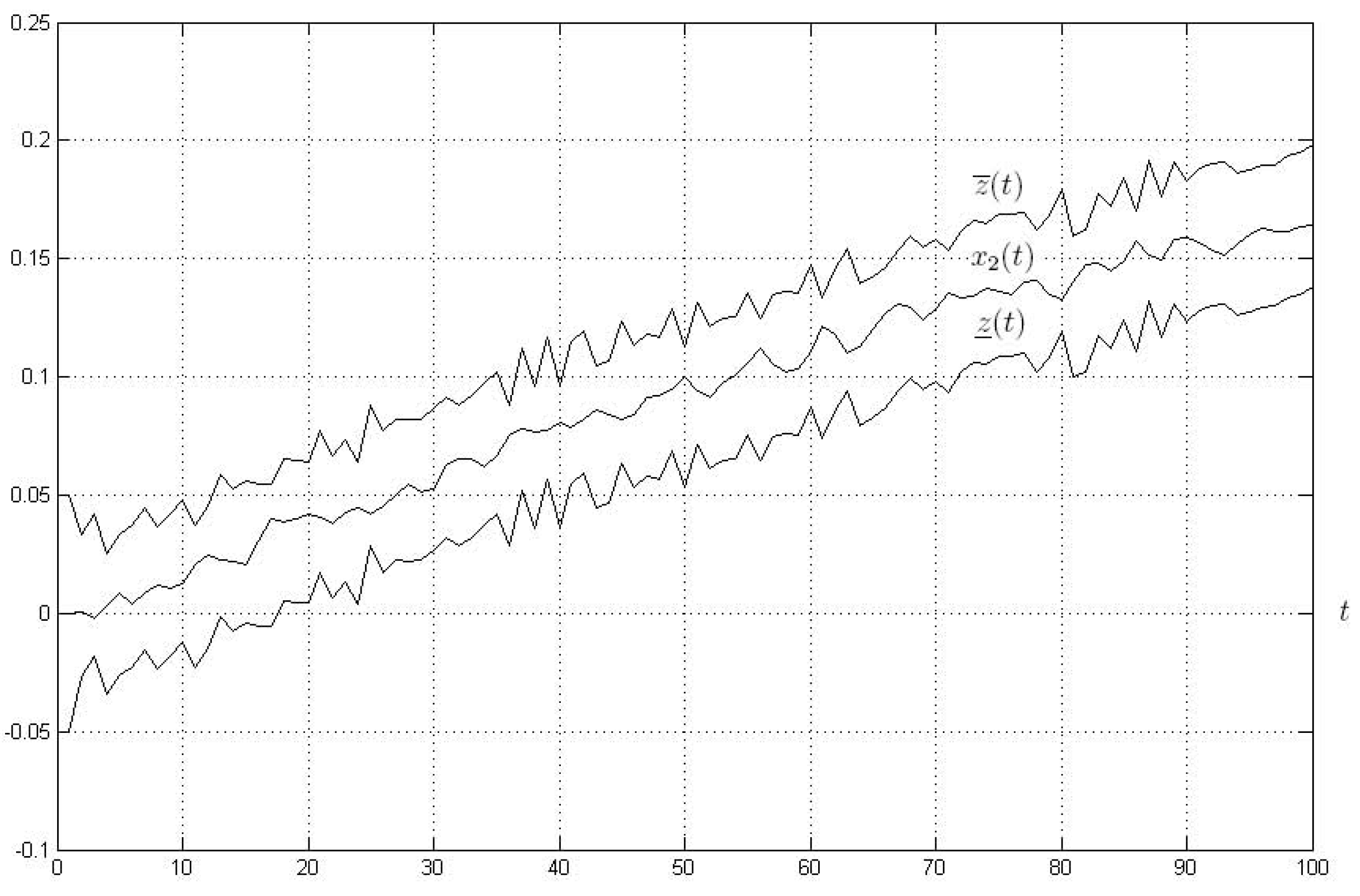
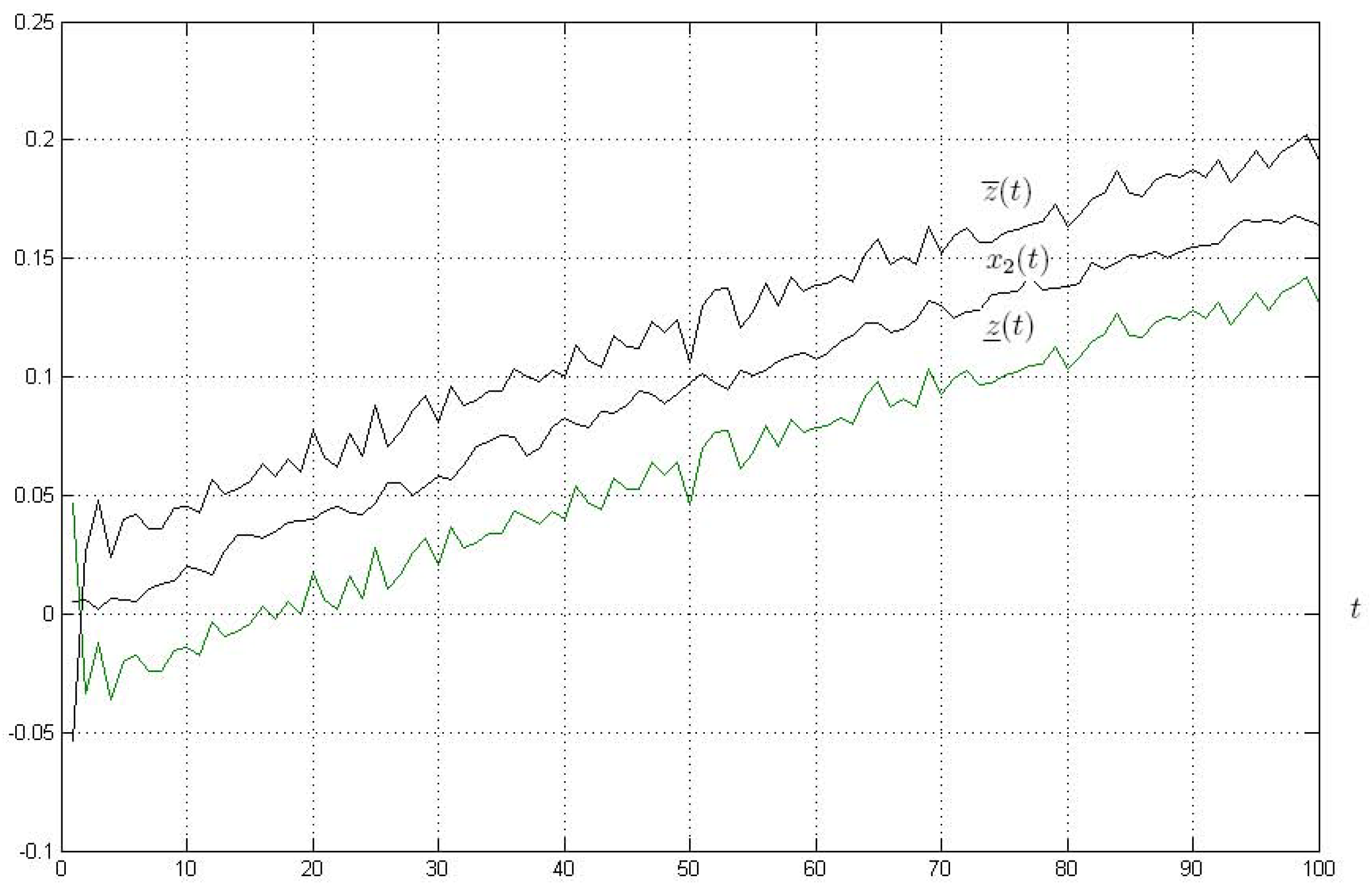
6. Interval Estimation of the Vector $x\left(t\right)$

The suggested approach to the interval estimation of the variable $z\left(t\right)$ can be used to obtain the estimate of the full vector $x\left(t\right)$ as follows. We assume that matrix H is of full row–rank and

$$H=\left(H_{0}0\right),y\left(t\right)=H_0{x}^{\left(1\right)}\left(t\right)+v\left(t\right),x\left(t\right)=\left(\begin{array}{c}\hfill x^{\left(1\right)}\left(t\right)\\ \hfill x^{\left(2\right)}\left(t\right)\end{array}\right),$$

$H_0$ is a nonsingular matrix. Let us define

$$\begin{array}{ccc}\hfill \underline{y}\left(t\right)& =& y\left(t\right)-E_l{v}_{\ast },\overline{y}\left(t\right)=y\left(t\right)+E_l{v}_{\ast },\hfill \\ \hfill {\underline{x}}^{\left(1\right)}\left(t\right)& =& H_0^{-1}\underline{y}\left(t\right),{\overline{x}}^{\left(1\right)}\left(t\right)=H_0^{-1}\overline{y}\left(t\right).\hfill \end{array}$$

(19)

Then

$$\begin{array}{ccc}\hfill {\underline{e}}^{\left(1\right)}\left(t\right)& =& x^{\left(1\right)}\left(t\right)-{\underline{x}}^{\left(1\right)}\left(t\right)=H_0^{-1}(y\left(t\right)-v\left(t\right))-H_0^{-1}\underline{y}\left(t\right)=H_0^{-1}(E_l{v}_{\ast }-v\left(t\right)),\hfill \\ \hfill {\overline{e}}^{\left(1\right)}\left(t\right)& =& {\overline{x}}^{\left(1\right)}\left(t\right)-x^{\left(1\right)}\left(t\right)=H_0^{-1}\overline{y}\left(t\right)-H_0^{-1}(y\left(t\right)-v\left(t\right))=H_0^{-1}(E_l{v}_{\ast }+v\left(t\right)).\hfill \end{array}$$

Assuming that $H_0^{-1}\ge 0$, it follows from $E_l{v}_{\ast }\pm v\left(t\right)\ge 0$ that ${\underline{e}}^{\left(1\right)}\left(t\right)\ge 0$, ${\overline{e}}^{\left(1\right)}\left(t\right)\ge 0$ and ${\underline{x}}^{\left(1\right)}\left(t\right)\le x^{\left(1\right)}\left(t\right)\le {\overline{x}}^{\left(1\right)}\left(t\right)$. As a result, the variable $x^{\left(1\right)}\left(t\right)$ under the condition $H_0^{-1}\ge 0$ is estimated based on (19) and the disturbance $\rho \left(t\right)$ does not affect this estimate.

Remark 4.

The condition $H_0^{-1}\ge 0$ is satisfied in practical important cases when the vector $x^{\left(1\right)}$ is measured by sensors and $H_0=H_0^{-1}=I_l.$

The estimate of the variable $x^{\left(2\right)}$ is given by the observer (12). Set $z\left(t\right):=x^{\left(2\right)}\left(t\right)=M^{\left(2\right)}x\left(t\right)$ for matrix $M^{\left(2\right)}$ and checks the condition (5) to clarify if it is possible to design the observer invariant with respect to the disturbance. Then depending on the results, one constructs an insensitive or robust observer.

7. Example

Consider the discrete-time model of the electric servo-actuator of the manipulator:

$$\begin{array}{ccc}\hfill x_1(t+1)& =& k_1{x}_2\left(t\right)+x_1\left(t\right),\hfill \\ \hfill x_2(t+1)& =& k_2{x}_3\left(t\right)+x_2\left(t\right)+\rho \left(t\right),\hfill \\ \hfill x_3(t+1)& =& k_3{x}_2\left(t\right)+k_4{x}_3\left(t\right)+k_{5}u\left(t\right),\hfill \\ \hfill y_1\left(t\right)& =& x_1\left(t\right)+v_1\left(t\right),\hfill \\ \hfill y_2\left(t\right)& =& x_3\left(t\right)+v_2\left(t\right),\hfill \end{array}$$

(20)

where the coefficients $k_1÷k_5$ describe the sampling time and the servo-actuator parameters; the addend $\rho \left(t\right)$ is explained by the external loading moment. The following matrices describe this model:

$$\begin{array}{ccc}\hfill F& =& \left(\begin{array}{ccc}1& k_1& 0\\ 0& 1& k_2\\ 0& k_3& k_4\end{array}\right),G=\left(\begin{array}{c}0\\ 0\\ k_5\end{array}\right),H=\left(\begin{array}{ccc}1& 0& 0\\ 0& 0& 1\end{array}\right),L=\left(\begin{array}{c}0\\ 1\\ 0\end{array}\right).\hfill \end{array}$$

Construct the interval observer estimating the variable $x_2\left(t\right)$ with $M=\left(010\right)$. Since the disturbance enters in the equation for $x_2\left(t\right)$, the model will be sensitive to the disturbance, and one may set in (9) $L^{\left(k\right)}=0$ and obtain with $k=1$ the equation

$$(\Phi -J_{\ast })\left(\begin{array}{ccc}1& k_1& 0\\ 0& 1& k_2\\ 0& k_3& k_4\\ 1& 0& 0\\ 0& 0& 1\end{array}\right)=0.$$

Its solution is $\Phi =(1/k_1-10)$ and $J_{\ast }=(1/k_1-k_2)$ that gives $G_{\ast }=0$ and $L_{\ast }=-1.$ It can be shown that condition (5) is satisfied and $H_z=-1$, $Q=(1/k_{1}0)$.

The model is given by

$$\begin{array}{ccc}\hfill x_{\ast }(t+1)& =& (1/k_1)H_{1}x\left(t\right)-k_2{H}_{2}x\left(t\right)-\rho \left(t\right),\hfill \\ \hfill z\left(t\right)& =& -x_{\ast }\left(t\right)+(1/k_1)y_1\left(t\right).\hfill \end{array}$$

The interval observer is based on this model and is described as follows:

$$\begin{array}{ccc}\hfill {\underline{x}}_{\ast }(t+1)& =& (1/k_1)y_1\left(t\right)-k_2{y}_2\left(t\right)-(1/k_1)v_{\ast 1}-k_2{v}_{\ast 2}-{\rho }_{\ast },\hfill \\ \hfill {\overline{x}}_{\ast }(t+1)& =& (1/k_1)y_1\left(t\right)-k_2{y}_2\left(t\right)+(1/k_1)v_{\ast 1}+k_2{v}_{\ast 2}+{\rho }_{\ast },\hfill \\ \hfill \underline{z}\left(t\right)& =& -{\overline{x}}_{\ast }\left(t\right)+(1/k_1)y_1\left(t\right),\hfill \\ \hfill \overline{z}\left(t\right)& =& -{\underline{x}}_{\ast }\left(t\right)+(1/k_1)y_1\left(t\right).\hfill \end{array}$$

(21)

The variables $x_1\left(t\right)$ and $x_3\left(t\right)$ can be estimated according to (19):

$$\begin{array}{ccc}\hfill {\underline{x}}_1\left(t\right)& =& y_1\left(t\right)-v_{\ast 1},{\underline{x}}_3\left(t\right)=y_2\left(t\right)-v_{\ast 2},\hfill \\ \hfill {\overline{x}}_1\left(t\right)& =& y_1\left(t\right)+v_{\ast 1},{\overline{x}}_3\left(t\right)=y_2\left(t\right)+v_{\ast 2}.\hfill \end{array}$$

Comparing the obtained results with those that were previously obtained for this example in [15] and other similar papers, one can conclude that the suggested approach gives a simpler observer and an interval with a smaller width.

Consider for the simulation, the model (20), and the observer (21); the control $u\left(t\right)=0.2sin(t/100),$ the measurement noises $v_1\left(t\right)$, $v_2\left(t\right)$, and $\rho \left(t\right)$ are random processes evenly distributed on $[-0.01,0.01]$. Set for simplicity $k_1=k_2=k_5=1,$$k_3=k_4=-1$; $v_{\ast 1}=v_{\ast 2}={\rho }_{\ast }=0.01$. Simulation results are shown in Figure 1 and Figure 2, where the functions $x_2\left(t\right)$ and its estimates $\underline{z}\left(t\right)$ and $\overline{z}\left(t\right)$ are presented for $x_{\ast }\left(0\right)=0$. In Figure 1, the initial conditions are ${\underline{x}}_{\ast }\left(0\right)=-0.05$ and ${\overline{x}}_{\ast }\left(0\right)=0.05$, in Figure 2 ${\underline{x}}_{\ast }\left(0\right)=0.05$ and ${\overline{x}}_{\ast }\left(0\right)=-0.05$. Crossing two graphs in Figure 2 corresponds to Remark 3.

8. Conclusions

The problem surrounding the interval observer design for dynamic systems (described by linear discrete-time models under disturbance and measurement noises) was studied in this paper. To solve the problem, the reduced order model of the initial system, which is invariant (or has minimal sensitivity) to the disturbance was used. Such a model is realized in the identification canonical form. The relations to design the interval observer of minimal dimension, which estimates the prescribed linear function of the state vector of the initial system, were obtained.

References

1. Edwards, C.; Spurgeon, S.; Patton, R. Sliding mode observers for fault detection and isolation. Automatica 2000, 36, 541–553. [Google Scholar] [CrossRef]
2. Fridman, L.; Levant, A.; Davila, J. Observation of linear systems with unknown inputs via high-order sliding-modes. Int. J. Syst. Sci. 2007, 38, 773–791. [Google Scholar] [CrossRef]
3. Zhirabok, A.; Zuev, A.; Seriyenko, O.; Shumsky, A. Fault identificaition in nonlinear dynamic systems and their sensors based on sliding mode observers. Autom. Remote Control 2022, 83, 214–236. [Google Scholar] [CrossRef]
4. Chebotarev, S.; Efimov, D.; Raissi, T.; Zolghadri, A. Interval observers for continous-time LPV systems with L1/L2 performance. Automatica 2015, 58, 82–89. [Google Scholar] [CrossRef]
5. Degue, K.; Efimov, D.; Richard, J. Interval observers for linear impulsive systems. IFAC-PapersOnLine 2016, 49-18, 867–872. [Google Scholar] [CrossRef]
6. Dinh, T.; Mazenc, F.; Niculescu, S. Interval observer composed of observers for nonlinear systems. In Proceedings of the 2014 European Control Conference (ECC), Strasbourg, France, 24–27 June 2014; pp. 660–665. [Google Scholar]
7. Kolesov, N.; Gruzlikov, A.; Lukoyanov, E. Using fuzzy interacting observers for fault diagnosis in systems with parametric uncertainty. In Proceedings of the XII-th International Symposium Intelligent Systems (INTELS’16), Moscow, Russia, 5–7 October 2016; pp. 499–504. [Google Scholar]
8. Mazenc, F.; Bernard, O. Interval observers for linear time-invariant systems with disturbances. Automatica 2011, 47, 140–147. [Google Scholar] [CrossRef] [Green Version]
9. Raissi, T.; Efimov, D.; Zolghadri, A. Interval state estimation for a class of nonlinear systems. IEEE Trans. Autom. Control 2012, 57, 260–265. [Google Scholar] [CrossRef]
10. Zheng, G.; Efimov, D.; Perruquetti, W. Interval state estimation for uncertain nonlinear systems. In Proceedings of the IFAC Nolcos 2013, Toulouse, France, 4–6 September 2013. [Google Scholar]
11. Zhirabok, A.; Zuev, A.; Kim Chung, I. A Method to design interval observers for linear time-invariant systems. Comput. Syst. Sci. Int. 2022, 61, 485–495. [Google Scholar] [CrossRef]
12. Efimov, D.; Perruquetti, W.; Raissi, T.; Zolghadri, A. Interval observers for time-varying discrete-time systems. IEEE Trans. Autom. Control 2013, 58, 3218–3224. [Google Scholar]
13. Mazenc, F.; Dinh, T.; Niculescu, S. Interval observers for discrete-time systems. Inter. J. Robust Nonlinear Control 2014, 24, 2867–2890. [Google Scholar] [CrossRef] [Green Version]
14. Efimov, D.; Polyakov, A.; Richard, J. Interval observer design for estimation and control of time-delay descriptor systems. Eur. J. Control 2015, 23, 26–35. [Google Scholar] [CrossRef]
15. Efimov, D.; Raissi, T. Design of interval state observers for uncertain dynamical systems. Autom. Remote Control 2015, 77, 191–225. [Google Scholar] [CrossRef]
16. Marouani, G.; Dinh, T.; Raissi, T.; Wang, X.; Messaoud, H. Unknown input interval observers for discrete-time linear switched systems. European J. Control 2021, 59, 165–174. [Google Scholar] [CrossRef]
17. Zammali, C.; Gorp, J.; Wang, Z.; Raissi, T. Sensor fault detection for switched systems using interval observer with L performance. Eur. J. Control 2020, 57, 147–156. [Google Scholar] [CrossRef]
18. Alives, J.; Moreno, J.; Davila, J.; Becerra, G.; Flores, F.; Chavez, C.; Marques, C. Stability radii-based interval observers for discrete-time nonlinear systems. IEEE Access 2022, 10, 3216–3227. [Google Scholar]
19. Blesa, J.; Rotondo, D.; Puig, V. FDI and FTC of wind turbines using the interval observer approach and virtual actuators/sensors. Control Eng. Pract. 2014, 24, 138–155. [Google Scholar] [CrossRef] [Green Version]
20. Rotondo, D.; Fernandez-Canti, R.; Tornil-Sin, S. Robust fault diagnosis of proton exchange membrane fuel cells using a Takagi-Sugeno interval observer approach. Int. J. Hydrogen Energy 2016, 41, 2875–2886. [Google Scholar] [CrossRef] [Green Version]
21. Zhang, K.; Jiang, B.; Yan, X.; Edwards, C. Interval sliding mode based fault accommodation for non-minimal phase LPV systems with online control application. Intern. J. Control 2019. [Google Scholar] [CrossRef]
22. Khan, A.; Xie, W.; Zhang, B.; Liu, L. Design and applications of interval observers for uncertain dynamical systems. IET Circuits Devices Syst. 2020, 14, 721–740. [Google Scholar] [CrossRef]
23. Khan, A.; Xie, W.; Zhang, B.; Liu, L. A survey of interval observers design methods and implementation for uncertain systems. J. Frankl. Inst. 2021, 358, 3077–3126. [Google Scholar] [CrossRef]
24. Gu, D.; Liu, L.; Duan, G. Functional interval observer for the linear systems with disturbances. IET Control Theory Appl. 2018, 12, 2562–2568. [Google Scholar] [CrossRef]
25. Haochi, C.; Jun, H.; Xudong, Z.; Xiang, M.; Ning, X. Functional interval observer for discrete-time systems with disturbances. Appl. Math. Comput. 2020, 383, 125352. [Google Scholar]
26. Liu, L.; Xie, W.; Khan, A.; Zhang, L. Finite-time functional interval observer for linear systems with uncertainties. IET Control Theory Appl. 2020, 14, 2868–2878. [Google Scholar] [CrossRef]
27. Meyer, L. Robust functional interval observer for multivariable linear systems. J. Dyn. Syst. Meas. Control 2019, 141, 094502. [Google Scholar] [CrossRef]
28. Zhirabok, A.; Shumsky, A.; Solyanik, S.; Suvorov, A. Fault detection in nonlinear systems via linear methods. Int. J. Appl. Math. Comput. Sci. 2017, 27, 261–272. [Google Scholar] [CrossRef] [Green Version]
29. Zhirabok, A. Disturbance decoupling problem: Logic-dynamic approach-based solution. Symmetry 2019, 11, 555. [Google Scholar] [CrossRef] [Green Version]
30. Zhirabok, A. The problem of invariance in nonlinear discrete-time dynamic systems. Symmetry 2020, 12, 1241. [Google Scholar] [CrossRef]
31. Low, X.; Willsky, A.; Verghese, G. Optimally robust redundancy relations for failure detection in uncertain systems. Automatica 1996, 22, 333–344. [Google Scholar]
Figure 1. Graphs of the variable x 2 ( t ) and its estimates z ̲ ( t ) and z ¯ ( t ) with x ̲ ( 0 ) = 0.05 and x ¯ ( 0 ) = 0.05 .
Symmetry 14 02131 g001
Figure 2. Graphs of the variable x 2 ( t ) and its estimates z ̲ ( t ) and z ¯ ( t ) with x ̲ ( 0 ) = 0.05 and x ¯ ( 0 ) = 0.05 .
Symmetry 14 02131 g002
Publisher’s Note: MDPI stays neutral with regard to jurisdictional claims in published maps and institutional affiliations.