Control Charts for Monitoring the Mean of Skew-Normal Samples

Abstract

The presence of asymmetric data in production processes or service operations has prompted the development of new monitoring schemes. In this article, an adapted version of the exponentially weighted moving averages (EWMA) control chart with dynamic limits is proposed to monitor the mean of samples from the skew-normal distribution. The detection ability of the proposed control chart in online monitoring was investigated by simulating the average run length (ARL) performance for different out-of-control scenarios. The results of the simulation study suggest that the proposed scheme overcomes the main drawback of the recently developed Shewhart-type control scheme. As shown in this article, the existing Shewhart-type procedure exhibits the undesirable property of taking longer to detect changes in the mean value of skewed normal observations due to increases in the shape parameter of the basic distribution than in stable conditions. The proposed control chart was shown to work fairly acceptably in all considered out-of-control scenarios.

1. Introduction

As stated by Arif and Aslam [1], control charts are the most widely used tool in Statistical Quality Control (SQC) to monitor and improve manufacturing processes in industry. Recently, the use of control charts for process improvement has been extended to the area of service operations. Khan et al. [2] see them as an effective procedure to identify variation patterns and to indicate when the process has changed due to some controllable or uncontrollable factors. In general, control charts can be used in repetitive processes.

Khan et al. [2] state that most of the processes that have traditionally been monitored with the help of control charts were designed, at least approximately, under the normal distribution assumption of the quality variable or the vector characterizing them. However, this assumption is not always realistic. In daily practice, especially in the early stages of monitoring, the normality of the available measurements is difficult to establish, and even if possible, normality is merely an assumption, as the quality variable can actually follow another non-normal distribution. When the normality assumption is fulfilled, and even in cases where departures from this requirement are not particularly severe, the $\overline{X}$ chart, for instance, may be suitable for monitoring process location. Otherwise, when the assumption of normality does not hold, the existing monitoring schemes perform poorly.

Many quality characteristics have asymmetric distributions, such as time-to-event variables. Different proposals have been developed for the monitoring of asymmetric data. Bai and Choi [3] proposed a heuristic method based on the concept of weighted variance to draw the control limits of the $\overline{X}$ and R charts in the case of skewed populations. Khoo et al. [4] proposed a synthetic control chart to monitor the mean in biased populations using a weighted variance based procedure. Karagz and Hamurkaroglu [5] proposed new control limits for the $\overline{X}$ and R charts for skewed distributions using weighted variance, weighted standard deviation, and skewness correction methods. Aako et al. [6] developed a Shewhart-type control chart to monitor data with positive bias that are assumed to come from the Marshall–Olkin inverse log-logistic distribution (MOILLD). Ahmed et al. [7] proposed a hybrid EWMA control chart based on a robust estimation procedure to monitor quality characteristics following symmetric, ( though not necessarily normal) as well as skewed data. None of the referred specialized literature deals with the specific topic of skew-normal distributed data.

The skew-normal distribution is one of the asymmetric distributions that has received the most attention in recent years. The preference for the use of this distribution is perhaps due to its close relationship with the normal distribution and its great flexibility for modeling a wide spectrum of asymmetric data. Figueredo and Gomes [8] proposed bootstrap control charts for monitoring any kind of changes in the mean and/or upward changes in the standard deviation when the quality variable belong to the univariate skew-normal family. This is a class of skew-normal models having the normal distribution as a particular member. The same authors present enhanced properties of the distributions in this class to motivate their use in practical applications, including the monitoring of univariate and bivariate industrial processes. To monitor skew-normal processes, bootstrap control charts are very useful, despite of the disadvantages of a highly time-consuming retrospective phase of analysis. Many papers (see, for instance, Seppala et al. [9], Liu and Tang [10], and Jones and Woodall [11]) have reported that for skewed distributions, bootstrap control charts have better performance on average than the conventional Shewhart-type ones.

Although Figueredo and Gomes [8] analyze the out-of-control performance of their proposed schemes, only processes with changes in the mean level and/or the dispersion for a fixed value of the shape parameter of the skew-normal distribution were of concern. The problem of changes in a process due to changes in the shape parameter was not addressed.

Tsai [12] derived an approximated distribution of the sample mean of skew-normal observations and suggested an $\overline{X}$ control chart based on it. This approximation, however, does not perform well when the distribution is highly skewed. Rather than approximating, Li et al. [13] derived the exact distributions of the sample mean and range and proposed Shewhart-type two-sided control charts to monitor the mean and spread of skewed normal data.

Through a simulation study, Li et al. [13] were able to establish that the false alarm rate (FAR) is maintained at the previously established nominal level for different values of the sample size and the shape parameter. Unfortunately, their study only takes into account the monitoring of the in-control process level for a fixed value of the parameter ruling the skewness of the basic distribution. That is, the scenarios under consideration only correspond to stable processes. The out-of-control performance of the proposed schemes was not addressed. As will be seen later, when the main goal of monitoring aims to detect increases in the mean of a skew-normal process due to an increase in the shape parameter of the basic model, Li’s proposal is not ARL-unbiased, that is, the schemes take longer to detect a change in the mean than they take to produce a false alarm.

To overcome the aforementioned drawback of Li’s methodology, this article proposes to build an exponentially weighted moving averages (EWMA) chart with probability limits to monitor changes in the skew-normal process mean. The resulting control methodology is an adapted version of the EWMA chart with the dynamic limits for Poisson counts in Phase II proposed by Shen et al. [14]. The new chart shows better overall performance in terms of lower out-of-control ARL in all considered scenarios.

The main distinguishing features of this work is the presentation of a monitoring scheme based on Shen’s proposal that allows detection of changes in the mean level of a skew-normal process that are exclusively due to changes in the asymmetry of the investigated process. The specificity of the work lies in the fact that the existing schemes do not address this problem and only deal with changes in the mean level of a skew-normal process that are due to changes in the location and/or scale parameters for a fixed value of the parameter ruling the asymmetry of the basic model. In addition, the proposed EWMA-type scheme seems to correct the undesirable property of not being ARL-unbiased, as Li’s chart for the mean is shown to be.

The rest of this article is organized as follows. Section 2 relates a few general issues concerning the skew-normal distribution. In Section 3, we present relevant insights related to chart design for monitoring the mean of skew-normal processes. Section 4 and Section 5 deal with specific aspects of the simulation study, then present and discuss the results obtained from it. In Section 6, an example with simulated samples is used to illustrate the design and performance of the proposed control schemes. Finally, in the last section, concluding remarks and recommendations are provided.

2. The Skew-Normal Distribution

In general, many real-life situations can be modeled using the normal distribution. However, certain random phenomena tend to behave in such a way that a presumed normal distribution is not quite enough to adequately represent them. Azzalini [15] proposed a class of probability density functions (PDF) that includes the standard normal distribution as a special case and provide better models to fit the available data, especially when the empirical distribution is close to normal while being slightly asymmetric.

Let X be a continuous random variable having a pdf of the form

$$f\left(x\right)=2\varphi \left(x\right)\mathsf{\Phi }\left(\lambda x\right),\lambda \in \mathbb{R}$$

(1)

where

$$\varphi \left(x\right)=\frac{1}{\sqrt{2\pi }}exp\left(-\frac{x^2}{2}\right)$$

(2)

and

$$\mathsf{\Phi }\left(\lambda x\right)=\underset{-\infty }{\overset{\lambda x}{\int }}\varphi \left(t\right)dt$$

(3)

denote the pdf of the standard normal distribution and its cumulative distribution function (cdf), respectively. The real constant, $\lambda$, is often referred to as the shape parameter, as it rules the direction and the magnitude of the skewness of the pdf (1). The asymmetry of the pdf (1) increases as $\lambda \to \pm \infty$, and is positive for $\lambda >0$ and negative for $\lambda <0$.

Now, let us define the variable $Y:=\xi +\omega X$, where $\xi \in \mathbb{R}$ and $\omega \in {\mathbb{R}}^{+}$. The random variable Y is said to follow a skew-normal distribution with a location parameter $\xi$, scale parameter $\omega$, and shape parameter $\lambda$. It can be briefly written as $Y\sim SN(\xi ,{\omega }^2,\lambda )$ to indicate that Y follows a skew-normal distribution. The standard skew-normal distribution is obtained if $\xi =0$ and $\omega =1$. It is easy to see that the univariate normal distribution $N(\xi ,{\omega }^2)$ is obtained when $\lambda =0$.

The expected value of the random variable Y is

$$E\left(Y\right)=\mu =\xi +\omega \delta \sqrt{\frac{2}{\pi }}$$

(4)

and the variance is

$$Var\left(Y\right)={\sigma }^2={\omega }^2\left(1-\frac{2{\delta }^2}{\pi }\right)$$

(5)

where $\delta =\frac{\lambda }{\sqrt{1+{\lambda }^2}}$.

More relevant insights about parameter estimation and inference in the context of the skew-normal distribution can be found in Azzalini [15,16] and Azzalini and Regoli [17]. Several enhanced properties that make the skew-normal distribution more suitable for modeling in practical applications can be found in Figueredo and Gomes [8].

3. Control Charts for the Mean of Skew-Normal Processes

3.1. Shewhart-Type Control Chart

Li et al. [13] proposed control charts for monitoring the mean level and dispersion of a skew-normal process with samples of size $n\ge 2$. Through simulations, they showed that the proposed schemes exhibit adequate performance in terms of the FAR for a fixed value of the sample size and the shape parameter. However, they do not address the problem of detecting process changes due to unwanted decreases in the shape parameter of the basic skew-normal model. For the purposes of this article, only a few of the theoretical results related to the design of the control charts for the mean level of Li’s methodology are presented. More details about the full control procedure can be found in Li et al. [13].

Suppose a univariate process characterized through the random variable $Y\sim SN(\xi ,{\omega }^2,\lambda )$, and let $\overline{Y}$ be a random variable denoting the mean of a sample of size $n\ge 2$ taken from the population Y and $\overline{Z}\sim SN\left(\lambda \right)$. For fixed $FAR=\alpha$ and $\lambda$ values, Li et al. [13] obtained the upper control limit (UCL) of the $\overline{Y}$ chart as

$$UCL=P\left(\overline{Y}<UCL\mid \mu ={\mu }_0,{\sigma }^2={\sigma }_0^2\right)=1-\frac{\alpha }{2},$$

(6)

where ${\mu }_0$ and ${\sigma }_0^2$ are the in-control mean and variance of the process, provided by (4) and (5), respectively. The relationship between $\overline{Y}$ and $\overline{Z}$ is set to be

$$\overline{Y}={\mu }_0+\left({\gamma }_1\overline{Z}+{\gamma }_2\right){\sigma }_0,$$

(7)

where ${\gamma }_1={\left(1-\frac{2{\delta }^2}{\pi }\right)}^{-1/2}$ and ${\gamma }_2=\sqrt{\frac{2}{\pi }}{\gamma }_1\delta$. As indicated in Section 2, the quantity $\delta$ depends on the shape parameter $\lambda$ of the basic model.

From (6) and (7), it is possible to find an expression of the form $P\left(\overline{Z}<{\overline{z}}_{\lambda ,n,\alpha }\right)=\alpha$, where ${\overline{z}}_{\lambda ,n,\alpha }$ is the $\alpha \times 100\%$ quantile of the distribution of $\overline{Z}$ and $n\ge 2$ is the size of the samples used for monitoring. For a given value of $\alpha$, the quantile ${\overline{z}}_{\lambda ,n,\alpha }$ is evaluated numerically from the sampling distribution of $\overline{Z}$, which is derived in the Appendix of Li et al. [13].

Thus, the upper (UCL) and lower (LCL) control limits of the $\overline{Y}$ chart are

$$\begin{array}{cc}\hfill UCL& \hfill ={\mu }_0+\left({\gamma }_1{\overline{z}}_{\lambda ,n,1-\alpha /2}+{\gamma }_2\right){\sigma }_0,\hfill \end{array}$$

$$\begin{array}{cc}\hfill LCL& \hfill ={\mu }_0+\left({\gamma }_1{\overline{z}}_{\lambda ,n,\alpha /2}+{\gamma }_2\right){\sigma }_0.\hfill \end{array}$$

(8)

In the case of the three sigma limits, it is assumed that $\alpha =0.0027$, thus, the UCL and LCL of the control chart can be written in the form

$$\begin{array}{cc}\hfill UCL& \hfill ={\mu }_0+A_1^U{\sigma }_0,\hfill \end{array}$$

$$\begin{array}{cc}\hfill LCL& \hfill ={\mu }_0-A_1^L{\sigma }_0.\hfill \end{array}$$

(9)

where $A_1^U=\left({\gamma }_1{\overline{z}}_{\lambda ,n,0.99865}+{\gamma }_2\right)$ and $A_1^L=\left({\gamma }_2-{\gamma }_1{\overline{z}}_{\lambda ,n,0.00135}\right)$. Li et al. [13] provide tables with the values of the charting constants $A_1^U$ and $A_1^L$ for different combinations of $\lambda$ and n values. Furthermore, a table for these same constants is provided when the parameters of the basic model are estimated.

3.2. The EWMAG-SN Control Chart

Shen et al. [14] first proposed an EWMA chart with probability control limits for monitoring Poisson count data with time-varying sample sizes in Phase II. This chart is called EWMAG, as it exhibits the appealing property of having geometrically-distributed run lengths, that is, the FAR of the control scheme does not depend on the monitoring time or on the size of the available samples.

Let $X_t$, $t=1,2,\dots$ be the count of an event during the fixed time period $(t-1,t]$. Given the sample size $n_t$, the variable $X_t$ independently follows the Poisson distribution with mean $\zeta n_t$, where $\zeta$ denotes the occurrence rate of the event of interest. To detect an abrupt change in the rate of occurrence from ${\zeta }_0$ to another unknown value ${\zeta }_1>{\zeta }_0$, it is proposed that the EWMA statistic

$$Q_j=(1-\theta )Q_{j-1}+\theta \frac{X_j}{n_j},j=1,2,3,...,t,$$

(10)

where $Q_0={\zeta }_0$ and $\theta \in (0;1]$ is the chart smoothing parameter. According to Shen et al. [14], the UCL $h_t$ of the EWMA statistic (10) at each monitoring moment t must satisfy

$$\begin{array}{c}\hfill P(Q_1>h_{1,\alpha }|n_1)=\alpha ,\\ \hfill P(Q_t>h_{t,\alpha }|Q_{t-1}<h_{t-1,\alpha },n_t)=\alpha ,t>1,\end{array}$$

(11)

where $\alpha$ is the previously established FAR level.

It is worth mentioning that the dynamic probability control limit $h_t$ is determined just after the $n_t$ value is observed at time t. Consequently, the EWMAG chart does not suffer from incorrect model assumptions on the mechanism generating the sizes of the available samples. Shen et al. [14] presented two equivalent computational procedures based on simulation via Monte Carlo and Markov chains to evaluate the conditional probabilities in (11).

In view of these attractive properties and the ease of implementation, this article proposes adapting the simulation-based algorithm in Shen et al. [14] for the special case of detecting changes in the mean of a skew-normal process due to changes in the shape parameter of the basic model. The rewriting of the complete algorithm is intentionally omitted; however, the introduction of required changes in it is guaranteed. For simplicity, we only point out that for a fixed $\alpha$ value of the FAR the algorithm focuses on finding the control limits at each monitoring moment $t=1,2,\dots$, as the $\frac{\alpha }{2}\times 100\%$ and $\left(1-\frac{\alpha }{2}\right)\times 100\%$ quantiles of the estimated in-control marginal distribution of the EWMA-type statistic

$$Q_j=(1-\theta )Q_{j-1}+\theta {\overline{Y}}_j,j=1,2,\dots ,t,$$

(12)

given that the process was in control at the preceding moment $t-1$. In (12), $0<\theta \le 1$ is the chart smoothing constant, ${\overline{Y}}_j$ is the mean of a sample with size n taken from a skew-normal process, and $Q_0={\mu }_0$, where ${\mu }_0$ is the in-control process mean calculated as indicated in (4).

The required marginal distribution at each monitoring moment t is obtained from a large enough number M of “pseudo-EWMA” values ${\widehat{Q}}_t$ that are simulated by generating the same quantity of random samples of size $n_t=n$ from the population $Y\sim SN({\xi }_0,{\omega }_0^2,{\lambda }_0)$, where ${\xi }_0$, ${\omega }_0$, and ${\lambda }_0$ are the target values of the basic model parameters. In order to ensure that the process works under stable conditions, each ${\widehat{Q}}_{t-1}$ value required for obtaining the respective pseudo-EWMA ${\widehat{Q}}_t$, $t\ge 2$ is randomly picked from the central $(1-\alpha )\times M$ values of the marginal distribution of the EWMA statistic estimated at moment $t-1$. For $t=1$, it is proposed that the estimation of the marginal distribution be obtained by making $Q_0={\mu }_0$.

After the corresponding control limit $h_t$ has been established at each monitoring moment t, the process stability is checked for the real observed ${\overline{Y}}_t$ value. The control procedure is followed as usual in online monitoring. For further discussion, the resulting control scheme is called the EWMAG-SN chart. For more details about the simulation-based algorithm, readers are referred to Shen et al. [14].

4. Simulation Study

4.1. Performance Evaluation

As usual, the performance of both the Shewhart-type and the proposed EWMAG-SN charts was evaluated in terms of the ARL, that is, the number of inspected samples before a control scheme first signals. To evaluate the performance of both the proposed procedures, a simulation-based study was conducted following the indications below.

4.2. Simulation Settings and Procedures

For all purposes, without loss of generality, the location and scale skew-normal parameters are set to be ${\xi }_0=0$ and ${\omega }_0=1$ and do not change throughout the study, even in out-of-control scenarios. To evaluate the impact of the shape parameter in chart performance, we explored the in-control target values ${\lambda }_0=0$ and ${\lambda }_0=1$. Both the Shewhart-type and the proposed EWMAG-SN charts described in Section 4 were calibrated to reach a nominal FAR of $\alpha =0.0027$. As for monitoring, it was assumed that samples are obtained sequentially and independently of each other, thus, the run lengths of each of the proposed schemes are geometrically distributed. As such, the in-control ARL formally represents the expectation of a geometric random variable. For the previously established nominal $\alpha$ value of the FAR, the in-control ARL is set to be approximately of 372 samples. Both the control charts were designed to only detect changes in the process mean due to current changes in the shape parameter of the skew-normal distribution.

Out-of-control scenarios were considered by introducing decreases and increases of different magnitudes in the skew-normal shape parameter. The explored out-of-control values of the skew-normal shape parameter ${\lambda }_1$ include changes expressed in integer multiples of 0.5 upward or downward from the in-control ${\lambda }_0$. The out-of-control ARL for each combination of impacting factors was estimated by computing the mean of 20,000 simulated run length values.

The ARL performance of Li’s chart was estimated for different values of the sample size n ranging from 2 to 5 with unitary increments. These settings coincide with some of those proposed by Li et al. [13] in their simulation study. For a given combination of n and ${\lambda }_0$ values, the corresponding in-control ARL was found as follows:

• Step 1. Evaluate the respective control limits by choosing the constants $A_1^U$ and $A_1^L$ in (9) from the tables provided by Li et al. [13] in the case of known process parameters.
• Step 2. Generate a sample of size n from the skew-normal distribution with parameters ${\xi }_0$, ${\omega }_0$ and ${\lambda }_0$.
• Step 3. Find the sample mean of the generated sample.
• Step 4. Compare the sample mean with the control limits. If the sample mean lies between the control limits, continue the sample generating process. Otherwise, stop.
• Step 5. Repeat steps 2 to 4 until the sample generating process first stops and count the number of generated samples. The obtained quantity is a run length value.
• Step 6. Repeat the preceding step a large number of times, say, 20,000, and evaluate the mean of all the obtained run length values. This is the estimated value of the in-control ARL.

To evaluate the out-of-control ARL performance, the algorithm described above must be implemented from the second step for each of the out-of-control values ${\lambda }_1$ in the set of those proposed to explore.

As stated before, theoretically speaking, the design of the EWMAG-SN requires neither special assumptions regarding the sample sizes themselves nor the mechanisms generating them. To ensure that both charts work under the same conditions, it is assumed that needed sample size $n_t=n$ at moment t is previously established at a known value among all of the explored ones. However, EWMAG-SN can be designed to deal with varying in time sample sizes as well. The fixed scenario as well as three others for varying sample sizes were used in Shen et al. [14] to show that the performance of the EWMAG chart does not depend on the mechanism generating the sample sizes.

The in-control ARL value of the EWMAG-SN scheme is achieved by setting $\theta =0.1$ in (12). For a given combination of the explored n and ${\lambda }_0$ values, the simulation-based algorithm with the variations that were needed to implement in the original version by Shen et al. [14] proceeds as follows:

• Step 1. Set the respective monitoring moment t. Generate a set of $M=50,000$ “pseudo EWMA” ${\widehat{Q}}_t$ values. Every ${\widehat{Q}}_{t,i}$, $i=1,\dots ,M$, value is calculated using (12) and is based on the mean of a sample of size n taken from $Y\sim SN({\xi }_0,{\omega }_0^2,{\lambda }_0)$. If $t=1$, set ${\widehat{Q}}_{0,i}={\mu }_0$, $i=1,\dots ,M$.
• Step 2. Sort the M pseudo-EWMA values ${\widehat{Q}}_{t,i}$ found in the preceding step in ascending order.
• Step 3. Pick the $\frac{\alpha }{2}\times M$ and $\left(1-\frac{\alpha }{2}\right)\times M$ quantiles of the sorted ${\widehat{Q}}_{t,i}$ values as the lower and the upper control limits $LC{L}_t$ and $UC{L}_t$, respectively.
• Step 4. Generate one sample of size n from $Y\sim SN({\xi }_0,{\omega }_0^2,{\lambda }_0)$, find the corresponding sample mean ${\overline{Y}}_t$, and evaluate the actual value of (12) based on ${\overline{Y}}_t$.
• Step 5. Compare the actual $Q_t$ value with the respective control limits. If it lies between the control limits, continue to the next monitoring moment $t+1$. Otherwise, stop the monitoring.
• Step 6. For $t\ge 2$, if it is decided to continue, retain the central $(1-\alpha )\times M$ values of the sorted ${\widehat{Q}}_{t,i}$ obtained in the preceding monitoring moment.
• Step 7. Pick one at random from the retained ${\widehat{Q}}_t$ sorted values to become the in-control ${\widehat{Q}}_{t-1,i}$ value every time it is necessary to obtain the M psuedo-EWMA values, as in Step 1, for the next monitoring moment.
• Step 8. Repeat steps 1 to 7 until the scheme first signals and count the number of generated samples. The obtained quantity is a run length value.
• Step 9. Repeat the preceding step a large number of times, say, 20,000, and take the mean of all the obtained run length values. This is the estimated value of the in-control ARL.

To evaluate the out-of-control performance of the EWMAG-SN chart, the above described algorithm must be implemented by generating the sample needed in Step 4 from $Y\sim SN({\xi }_0,{\omega }_0^2,{\lambda }_1)$.

5. Results and Discussion

Li et al. [13] report undeniably better performance in terms of the FAR in Phase II when the charts they propose are compared with the other existing control schemes under consideration. However, interesting insights concerning the performance in Phase II of Li’s $\overline{Y}$ chart for skew-normal samples that were obtained in our simulation study are addressed below.

First of all,

Table 1. Approximated in-control ARL performance of Li’s $\overline{Y}$ chart for $\alpha =0.0027$, ${\xi }_0=0$, ${\omega }_0=1$, and different n and ${\lambda }_0$ values.

In-Control	Sample Sizes
Shape, ${\mathit{\lambda }}_0$	$\mathit{n}=2$	$\mathit{n}=3$	$\mathit{n}=4$	$\mathit{n}=5$
0.0	366.06	363.69	365.81	367.16
0.5	365.88	366.10	368.10	368.18
1.0	370.21	374.55	371.48	369.05
1.5	372.08	376.10	374.24	375.15
2.0	373.52	371.55	374.15	371.24
2.5	372.46	373.58	372.06	373.45
3.0	372.23	373.33	374.18	370.68

shows the in-control ARL values of Li’s three-sigma $\overline{Y}$ chart for ${\xi }_0=0$, ${\omega }_0=1$, and different combinations of sample sizes and in-control values of the skew-normal shape parameter. These are the same combinations of values that were considered by Li et al. [13] in their study.

As can be seen, the results reported in Table 1 suggest a slight decrease in the nominal value of the in-control ARL for the smallest values of the sample size and the in-control skew-normal parameter, among those considered. Although this fact is only observed in a few cases and may be due to the simulation procedure itself, the results presented below are more serious.

Unfortunately, as far as can be understood, no results are reported by Li et al. [13] about the out-of-control performance of the proposed schemes, meaning that the problem concerning chart detection abilities remains unaddressed. If the main objective of the aforementioned research work consisted in presenting a methodology to allow the monitoring of asymmetric processes, then it should take into account the ability of the proposed charts to detect changes in the process mean, at least, for instance, those due to changes in any of the parameters of the basic model, including the shape parameter.

Table 2. Approximated ARL performance of Li’s $\overline{Y}$ chart designed for $\alpha =0.0027$, ${\xi }_0=0$, ${\omega }_0=1$, ${\lambda }_0=0$, and different n values.

Shape	Process	Sample Sizes
Parameter, $\mathit{\lambda }$	Mean, $\mathit{\mu }$	$\mathit{n}=2$	$\mathit{n}=3$	$\mathit{n}=4$	$\mathit{n}=5$
−2.00	−0.71	186.52	99.24	57.60	35.56
−1.50	−0.66	187.93	102.94	62.56	39.76
−1.00	−0.56	196.28	115.14	76.62	51.98
−0.50	−0.36	243.90	175.97	135.01	105.66
0.00	0.00	368.25	370.09	370.35	369.54
0.50	0.36	244.71	175.60	135.74	105.38
1.00	0.56	194.32	116.50	75.27	51.18
1.50	0.66	186.94	102.74	62.50	39.86
2.00	0.71	184.27	99.74	58.20	35.82

and

Table 3. Approximate ARL performance of Li’s $\overline{Y}$ chart designed for $\alpha =0.0027$, ${\xi }_0=0$, ${\omega }_0=1$${\lambda }_0=1$, and different n values.

Shape	Process	Sample Sizes
Parameter, $\mathit{\lambda }$	Mean, $\mathit{\mu }$	$\mathit{n}=2$	$\mathit{n}=3$	$\mathit{n}=4$	$\mathit{n}=5$
−2.00	−0.71	5.01	2.65	1.76	1.37
−1.50	−0.66	5.24	2.90	1.96	1.51
−1.00	−0.56	6.02	3.46	2.38	1.83
−0.50	−0.36	8.07	5.13	3.67	2.84
0.00	0.00	17.68	13.00	9.98	8.16
0.50	0.36	75.57	67.27	59.56	53.51
1.00	0.56	369.15	376.03	377.35	369.64
1.50	0.66	672.38	655.79	614.12	532.36
2.00	0.71	713.53	668.03	606.99	520.36

present the ARL performance of Li’s $\overline{Y}$ chart when changes in the process mean are due exclusively to changes in the skew-normal shape parameter for different values of n. Current changes in the shape parameter included out-of-control values ranging from $-2.0$ to $2.0$ in increments of $0.5$ for a fixed value ${\lambda }_0$. All schemes were calibrated to reach a nominal in-control ARL of 372.

Table 2 shows the results for ${\xi }_0=0$, ${\omega }_0=1$, and ${\lambda }_0=0$. In this case, the process is symmetric and the in-control mean and variance are ${\mu }_0=0$ and ${\sigma }_0^2=1$, respectively. That is, the goal is to detect a change from the mean of a normal symmetric process to an asymmetric one with the $\overline{Y}$ chart designed for ${\lambda }_0=0$. It can be observed that the chart detects both the increase and the decrease of the same magnitude at practically the same monitoring moment. Additionally, it can be observed that when the the change in the shape parameter and the sample size is larger, the chart performs the better. For example, while the chart takes approximately 194 samples to detect the increase in the process mean from ${\mu }_0=0.00$ to ${\mu }_1=0.66$ (which is due to an increase in the shape parameter from ${\lambda }_0=0.00$ to ${\lambda }_1=1.00$) with samples of size $n=2$, it takes 51 to detect the same change with samples of size $n=5$. Something very similar happens when trying to detect the decrease in the process mean from ${\mu }_0=0.00$ to ${\mu }_1=-0.66$ (which is due to a decrease in the shape parameter from ${\lambda }_0=0.00$ to ${\lambda }_1=-1.00$). A change to ${\mu }_1=1.50$ (or $-1.50$), for instance, takes less time to be detected than a change to ${\mu }_1=1.00$ (or $-1.00$). The in-control state is shown in Table 2 for $\lambda =0$ and $\mu =0$.

However, the simulations carried out here suggest a very different situation when ${\xi }_0=0$, ${\omega }_0=1$, and ${\lambda }_0=1$. The fact is that when the main goal of monitoring is to detect increases in the mean due to increases in the skew-normal shape parameter from an asymmetric process to a more asymmetric one, Li’s chart for the mean is not as efficient as when detecting changes from a normal symmetric process. Here, we analyze the out-of-control ARL performance of the Li’s $\overline{Y}$ chart when ${\lambda }_0=1$. In this case, the in-control process is clearly positively asymmetric with ${\mu }_0=0.56$ and ${\sigma }_0^2=0.68$. In Table 3, the results for ${\xi }_0=0$, ${\omega }_0=1$ and ${\lambda }_0=1$ are reported. It is easy to realize that the chart takes much longer to detect increases in the mean value than in the in-control case for all considered sample sizes. This means that Li’s $\overline{Y}$ chart is not ARL-unbiased.

We now discuss the results that were obtained for the same combinations of simulation settings in the case of the EWMAG-SN chart.

Table 4. Approximate ARL performance of the EWMAG-SN chart with $\theta =0.1$ for $\alpha =0.0027$, ${\xi }_0=0$, ${\omega }_0=1$, and different n and ${\lambda }_0$ values.

Shape	Process	${\mathit{\lambda }}_0=0$		${\mathit{\lambda }}_0=1$
Parameter, $\mathit{\lambda }$	Mean, $\mathit{\mu }$	$\mathit{n}=1$	$\mathit{n}=2$	$\mathit{n}=1$	$\mathit{n}=2$
−2.00	−0.71	15.62	7.36	3.01	1.35
−1.50	−0.66	17.52	8.38	3.18	1.47
−1.00	−0.56	27.71	11.92	3.72	1.95
−0.50	−0.36	52.48	26.85	5.54	2.93
0.00	0.00	368.32	367.87	13.45	7.33
0.50	0.36	52.16	25.45	61.91	40.14
1.00	0.56	26.28	11.13	368.13	368.53
1.50	0.66	17.36	8.17	329.38	210.83
2.00	0.71	15.46	7.54	253.96	176.81

shows the results for $\lambda =0$ and ${\lambda }_0=1$, including those for $n=1$. The results obtained for larger explored values of the sample size are intentionally omitted, as they are quite similar to those obtained for $n=2$, in the sense that they maintain the same trend in efficiency as those reported in the table. The table includes the results for $n=1$ in order to show that the EWMAG-SN can deal with individual observations as well. Li’s proposal was thought to deal with samples of size $n\ge 2$.

It is easy to see that the EWMAG-SN chart detects a specific current change in the skew-normal shape parameter substantially faster than Li’s chart does. For instance, the EWMAG-SN detects the planned increase (or decrease) of magnitude 0.5 from ${\lambda }_0=0$ in an average number of samples that is approximately ten times smaller ($AR{L}_1\approx 27$) than that of the Li’s chart ($AR{L}_1\approx 245$) when both schemes deal with a sample of size $n=2$. In addition, larger increases from ${\lambda }_0=0$ are detected drastically faster by the EWMAG-SN chart for a fixed n. This shows the high effectiveness of the proposed scheme for detecting any kind of changes in the skew-normal shape parameter.

Furthermore, the reported results in Table 4 suggest that EWMAG-SN seems to be an ARL-unbiased scheme when detecting changes from an in-control asymmetric state is desired. For instance, the increase from ${\lambda }_0=1$ to ${\lambda }_1=1.5$ is detected in an average number of samples that is smaller ($AR{L}_1\approx 211$) than the nominal $AR{L}_0=372$ with a sample of size $n=2$. Under the same conditions, Li’s chart requires slightly less than twice the nominal in-control ARL ($AR{L}_1\approx 672$).

6. Example

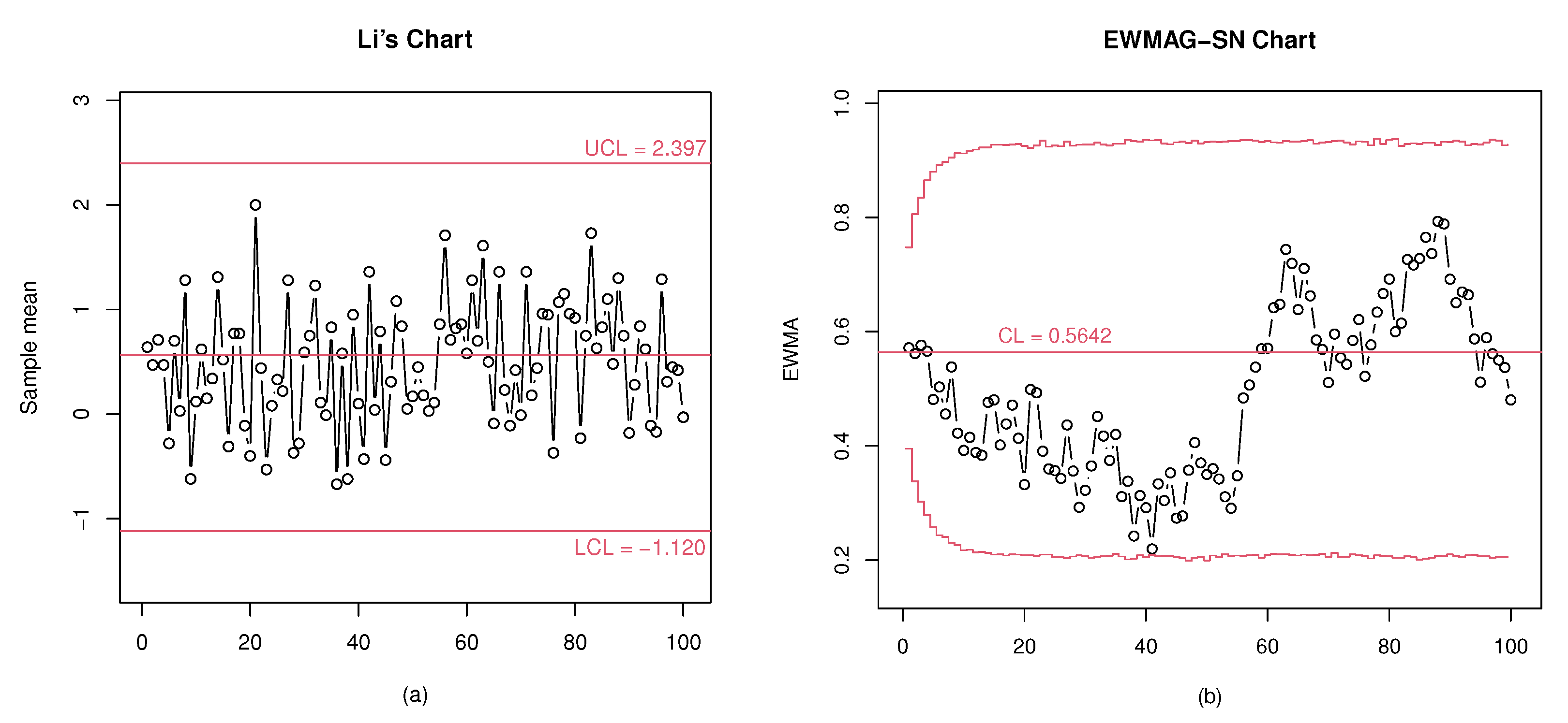
In the following, an example based on a set of simulated skew-normal samples is presented in order to illustrate the design and performance of the investigated control schemes. Both the charts were calibrated to reach a nominal FAR value of $\alpha =0.0027$. For this propose, 100 in-control samples of size $n=2$ were generated from a skew-normal process with a location parameter ${\xi }_0=0$, scale parameter ${\omega }_0=1$, and shape parameter ${\lambda }_0=1$. These settings yield a mean level of ${\mu }_0=0.5642$ when the process works under stable conditions.

According to Li’s proposal, the required values of the constants $A_1^L$ and $A_1^U$ in (9) satisfying the desired FAR level were taken from the table provided by the authors for the case of known in-control parameters and $n=2$. Thus, the control limits were set as $LCL=-1.120$ and $UCL=2.394$, respectively. The EWMAG-SN was designed for $\theta =0.1$ as the chart smoothing parameter. The control limits of the EWMAG-SN chart were approximated for the given FAR level by generating $M=100,000$ in-control psuedo-EWMA values at each monitoring moment. The schemes are shown in Figure 1. As can be seen, neither of the proposed charts present any evidence that something wrong is happening in the process.

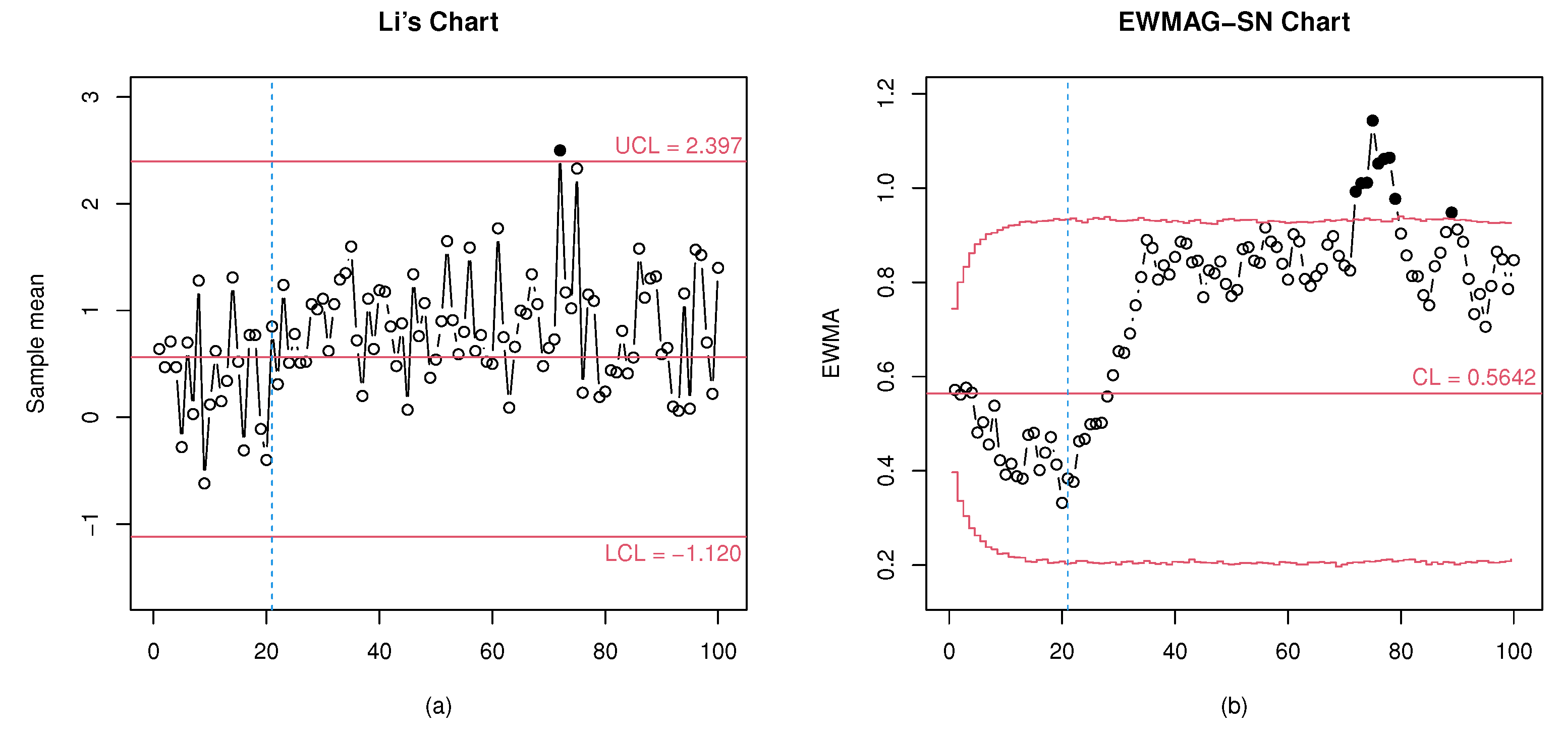
We are now left with the first 20 samples of the in-control process. From the 21st monitoring instant, it is proposed that 80 additional samples of size $n=2$ be generated from a skew-normal process with ${\xi }_1={\xi }_0=0$, ${\omega }_1={\omega }_0=1$, and ${\lambda }_1=1$. This yields a new value ${\mu }_1=0.7136$ for the mean level. This implies that the process experienced an increase in the mean that is exclusively due to an increase in the shape parameter of the basic distribution. The respective schemes are shown in Figure 2. The blue dashed line shows the shifting point in the sampling sequence.

As can be observed in Figure 2, Li’s chart only signals at the 72nd monitoring moment, while the EWMAG-SN chart shows alarms in samples 72 up to 79 as well as 89. If it were not for the single true signal of Li’s chart, it could be said that the pattern of dots it exhibits is more consistent with that of an in-control process. Meanwhile, although the EWMAG-SN chart begins signaling at the same time as Li’s chart, the shift in the mean level of theprocess is evident much earlier.

7. Conclusions and Recommendations

Li et al. [13] have proposed a methodology for monitoring the mean level and the dispersion of skew-normal processes that has been proven to work acceptably well in terms of the FAR for a fixed value of the shape parameter of the basic model. Although they authors do not address the out-of-control performance of their proposed methodology, we feel that it may be suitable for monitoring changes in the mean and the dispersion of skew-normal processes due to changes in the location and/or the scale parameter for a fixed stable value of the shape parameter.

Through our simulations, it was possible to show in this article that at least the chart for the mean level of Li’s methodology in Phase II suffers from the undesirable property of not being ARL-unbiased when increases in the process mean are only due to increases in the shape parameter of the skew-normal basic model. That is, Li’s chart takes longer to detect an increase (small in most cases) in the process mean than it takes to emit an alarm signal that is known to be false. This fact has serious implications in practical applications. In a real-life monitoring situation, it is not possible to know in advance the kind of changes that will take place in a process. If monitoring is being carried out with the assistance of Li’s chart, a small change in the process asymmetry will not be detected with a high probability by the scheme. Thus, the use of this methodology is not recommended unless there is some indication of what is causing or could cause process instability.

To overcome the drawbacks of the Li’s chart for monitoring the mean of skew-normal processes, it is recommended to use the EWMAG-SN chart instead. The simulation study carried out in this paper suggests that the EWMA-SN chart does not suffer from a lack of ARL-unbiasedness, at least when changes in the process mean are due solely to changes in the shape parameter of the basic model.

References

- Aris, O.H.; Aslam, M. A new generalized range control chart for the Weibull distribution. Complexity 2018, 2018, 9453589. [Google Scholar] [CrossRef]
- Khan, N.; Aslam, M.; Aldosari, M.S.; Jun, C. A multivariate control chart for monitoring several exponential quality characteristics using EWMA. IEEE Access 2018, 6, 70349–70358. [Google Scholar] [CrossRef]
- Bai, D.S.; Choi, I.S. X¯ and R charts for skewed populations. J. Qual. Technol. 1995, 27, 120–131. [Google Scholar] [CrossRef]
- Khoo, M.B.C.; Atta, A.M.A.; Wu, Z. A multivariate synthetic control chart for monitoring the process mean vector of skewed populations using weighted standard deviations. Commun. Stat.-Comput. 2009, 38, 1493–1518. [Google Scholar] [CrossRef]
- Karagoz, D.; Hamurkaroglu, C. Control charts for skewed distributions. Metod. Zv. 2012, 9, 95–106. [Google Scholar] [CrossRef]
- Aako, O.; Adewara, J.; Adekeye, K.; Nkemnole, E. X¯ and R control charts based on Marshall-Olkin inverse log-logistic distribution for positive skewed data. Afr. J. Pureand Appl. Sci. 2020, 1, 9–16. [Google Scholar] [CrossRef]
- Ahmed, A.; Sanaullah, A.; Hanif, M. A robust alternate to the HEWMA control chart under non-normality. Qual. Technol. Quant. Manag. 2020, 17, 423–447. [Google Scholar] [CrossRef]
- Figueredo, F.; Gomes, M.I. The skew-normal distribution in SPC. REVSTAT- J. 2013, 11, 83–104. [Google Scholar]
- Seppala, T.; Moskowitz, H.; Plante, R.; Tang, J. Statistical process control via the subgroup bootstrap. J. Qual. 1995, 27, 139–153. [Google Scholar] [CrossRef]
- Liu, R.Y.; Tang, J. Control charts for dependent and independent measurements based on the bootstrap. J. Am. Assoc. 1996, 91, 1694–1700. [Google Scholar] [CrossRef]
- Jones, L.A.; Woodall, W.H. The performance of bootstrap control charts. J. Qual. Technol. 1998, 30, 362–375. [Google Scholar] [CrossRef]
- Tsai, T.R. Skew normal distribution and the design of control charts for averages. Int. J. Reliab. Qual. Saf. Eng. 2007, 14, 49–63. [Google Scholar] [CrossRef]
- Li, C.; Su, N.C.; Su, P.F.; Shyr, Y. The design of X¯ and R control charts for skew-normal distributed data. Commun. Stat.-Methods 2014, 43, 4908–4924. [Google Scholar] [CrossRef]
- Shen, X.; Zou, C.; Jiang, W.; Tsung, F. Monitoring Poisson count data with probability control limits when sample sizes are time varying. Naval Res. Logist. 2013, 60, 625–636. [Google Scholar] [CrossRef]
- Azzalini, A. A class of distributions which includes the normal ones. Scand. J. Stat. 1985, 12, 171–178. [Google Scholar]
- Azzalini, A. Further results on a class of distributions which includes the normal ones. Statistica 1986, XLVI, 199–208. [Google Scholar]
- Azzalini, A.; Regoli, G. Some properties of skew-symmetric distributions. Ann. Inst. Stat. Math. 2012, 64, 857–879. [Google Scholar] [CrossRef] [Green Version]
Figure 1.
Control charts for the in-control skew-normal process with , , , and .
Figure 2.
Control charts for the artificially created out-of-control situation of .