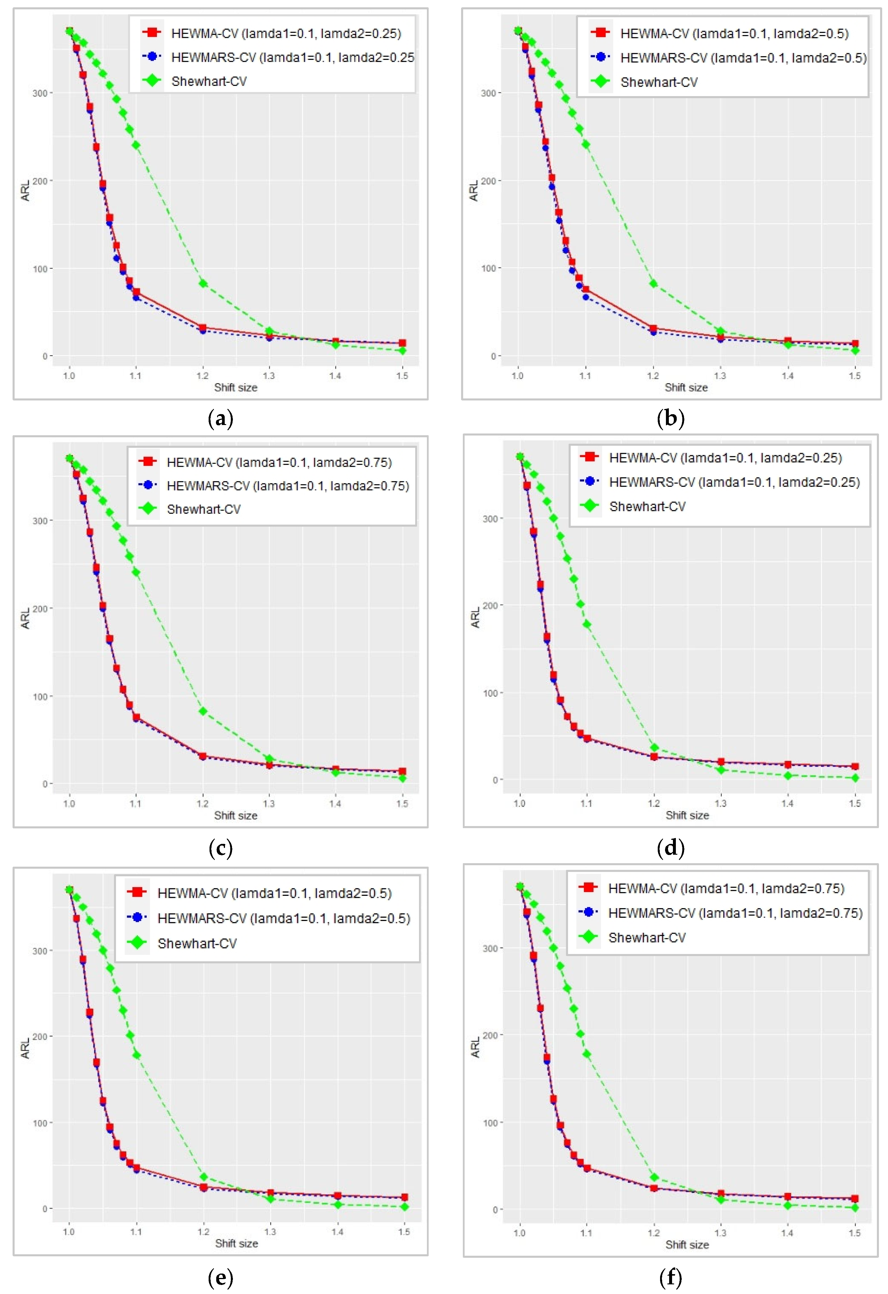
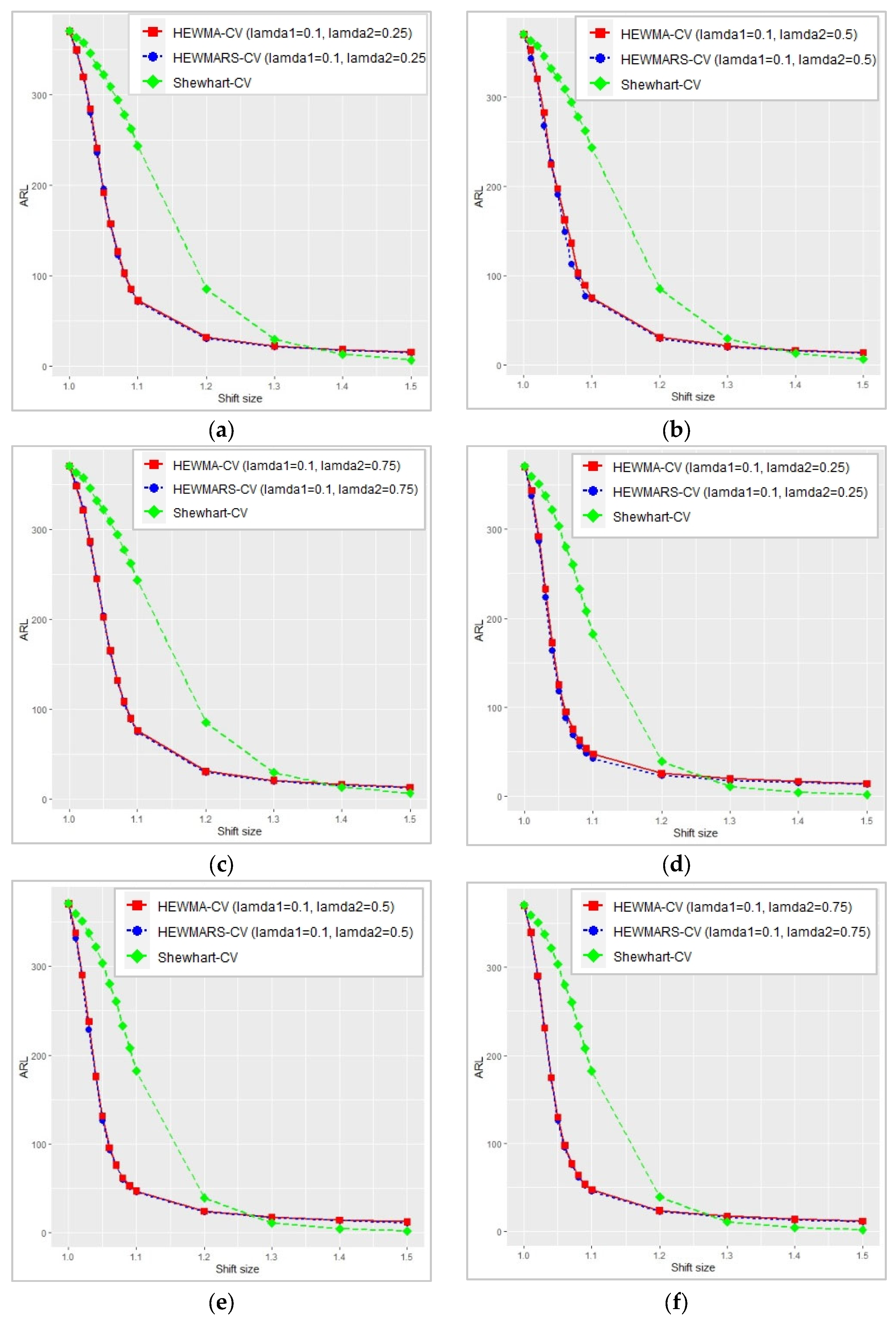
Figure 1.
Comparison of ARL between HEWMARS-CV, HEWMA-CV, and Shewhart Control Charts when the CV parameter = 0.08, the exponential smoothing parameter and various values of and the sample size is. (a) and n = 10; (b) and n = 10; (c) and n = 10; (d) and n = 20; (e) and n = 20; (f) and n = 20.
Figure 1.
Comparison of ARL between HEWMARS-CV, HEWMA-CV, and Shewhart Control Charts when the CV parameter = 0.08, the exponential smoothing parameter and various values of and the sample size is. (a) and n = 10; (b) and n = 10; (c) and n = 10; (d) and n = 20; (e) and n = 20; (f) and n = 20.
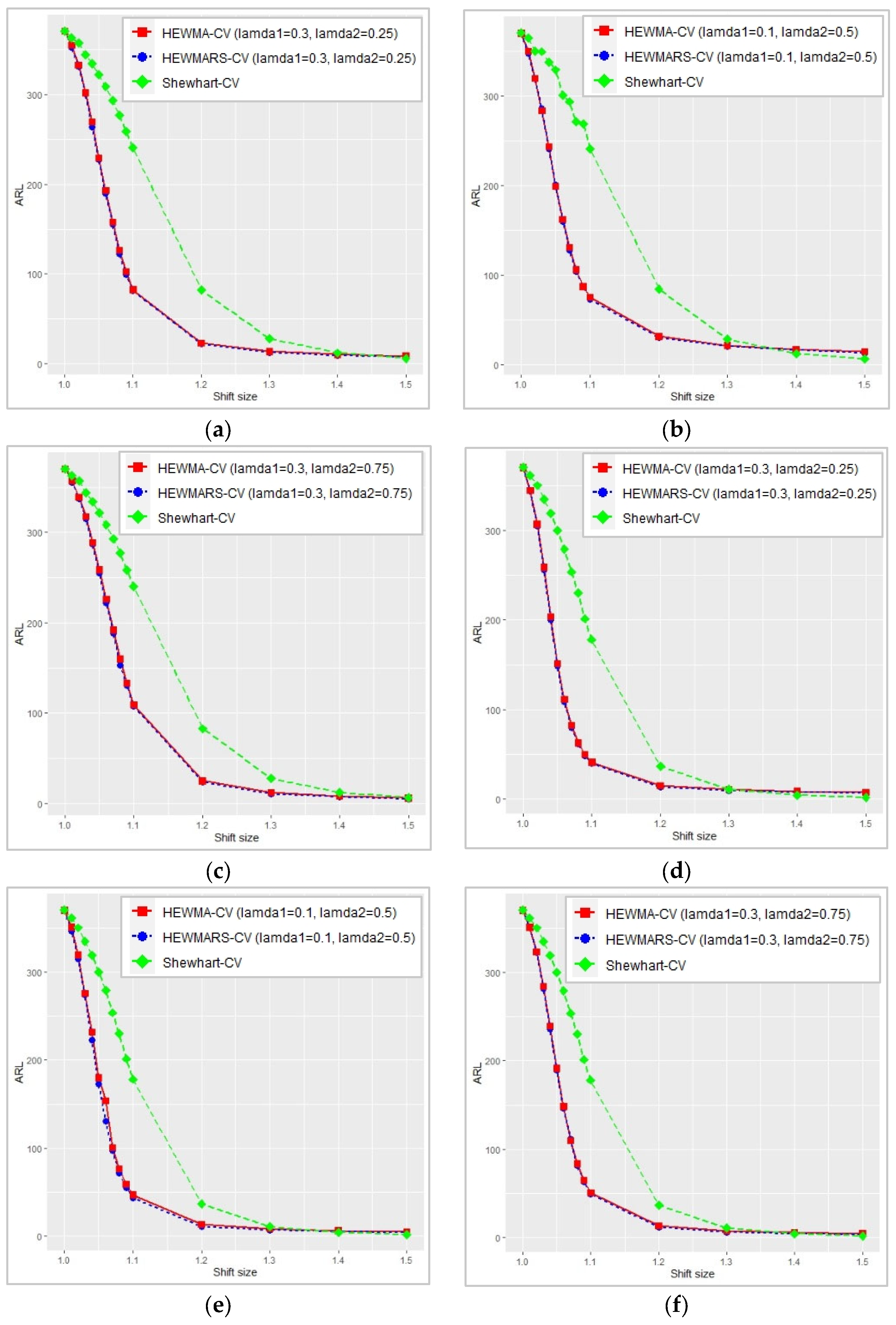
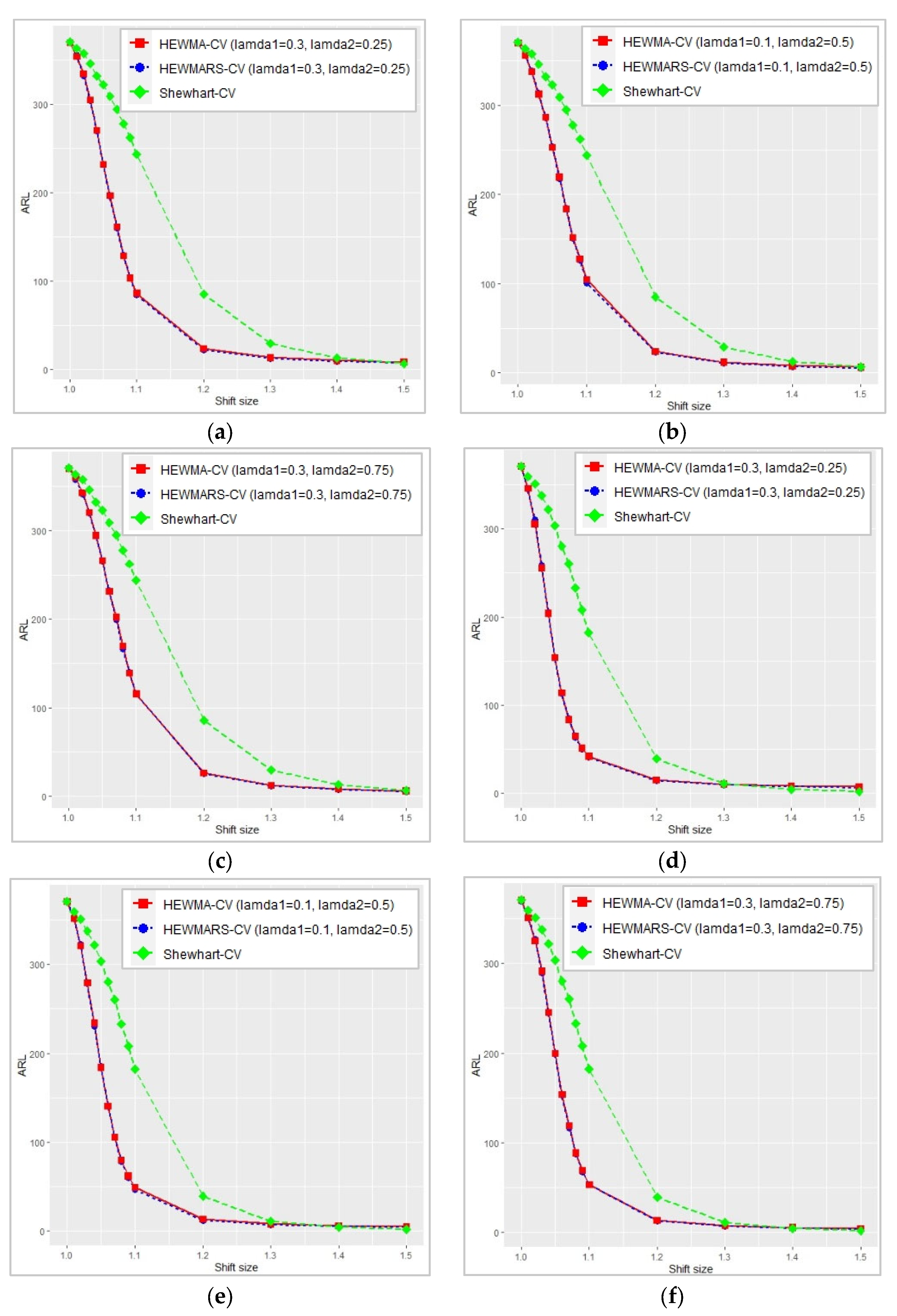
Figure 2.
Comparison of ARL between HEWMARS-CV, HEWMA-CV, and Shewhart Control Charts when the CV parameter = 0.08, the exponential smoothing parameter and various values of and the sample size is. (a) and n = 10; (b) and n = 10; (c) and n = 10; (d) and n = 20; (e) and n = 20; (f) and n = 20.
Figure 2.
Comparison of ARL between HEWMARS-CV, HEWMA-CV, and Shewhart Control Charts when the CV parameter = 0.08, the exponential smoothing parameter and various values of and the sample size is. (a) and n = 10; (b) and n = 10; (c) and n = 10; (d) and n = 20; (e) and n = 20; (f) and n = 20.
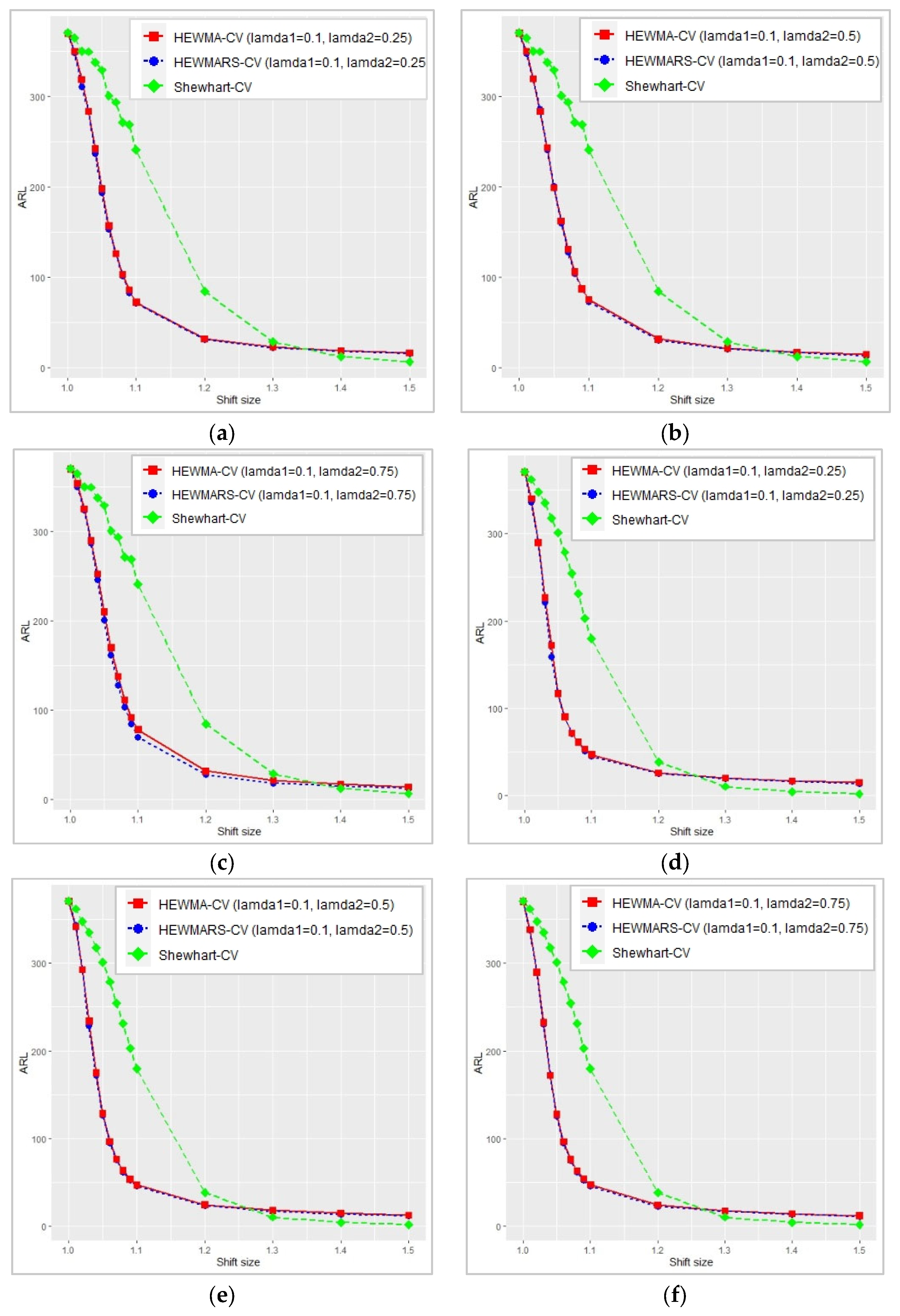
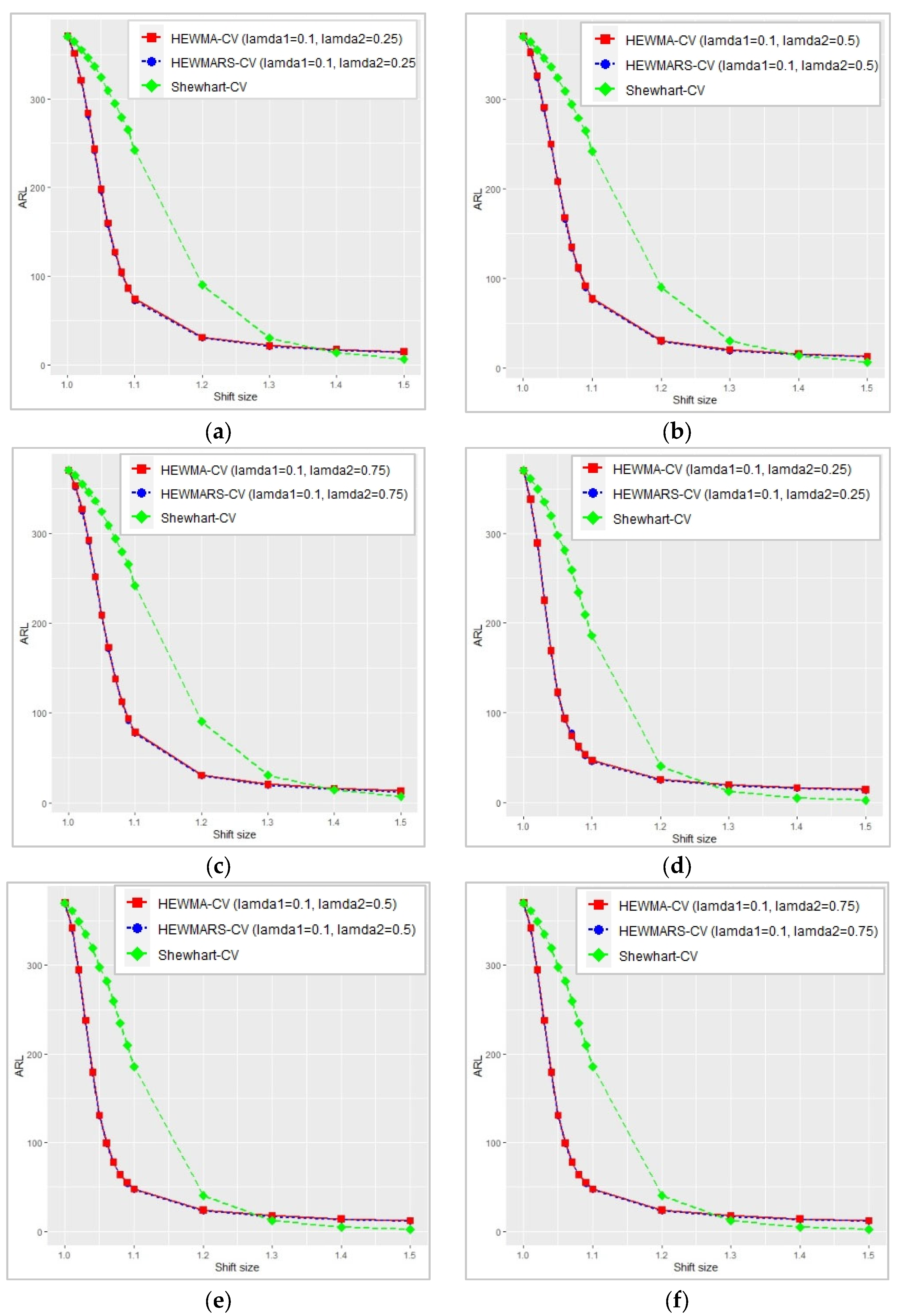
Figure 3.
Comparison of ARL between HEWMARS-CV, HEWMA-CV, and Shewhart Control Charts when the CV parameter = 0.10, the exponential smoothing parameter and various values of and the sample size is. (a) and n = 10; (b) and n = 10; (c) and n = 10; (d) and n = 20; (e) and n = 20; (f) and n = 20.
Figure 3.
Comparison of ARL between HEWMARS-CV, HEWMA-CV, and Shewhart Control Charts when the CV parameter = 0.10, the exponential smoothing parameter and various values of and the sample size is. (a) and n = 10; (b) and n = 10; (c) and n = 10; (d) and n = 20; (e) and n = 20; (f) and n = 20.
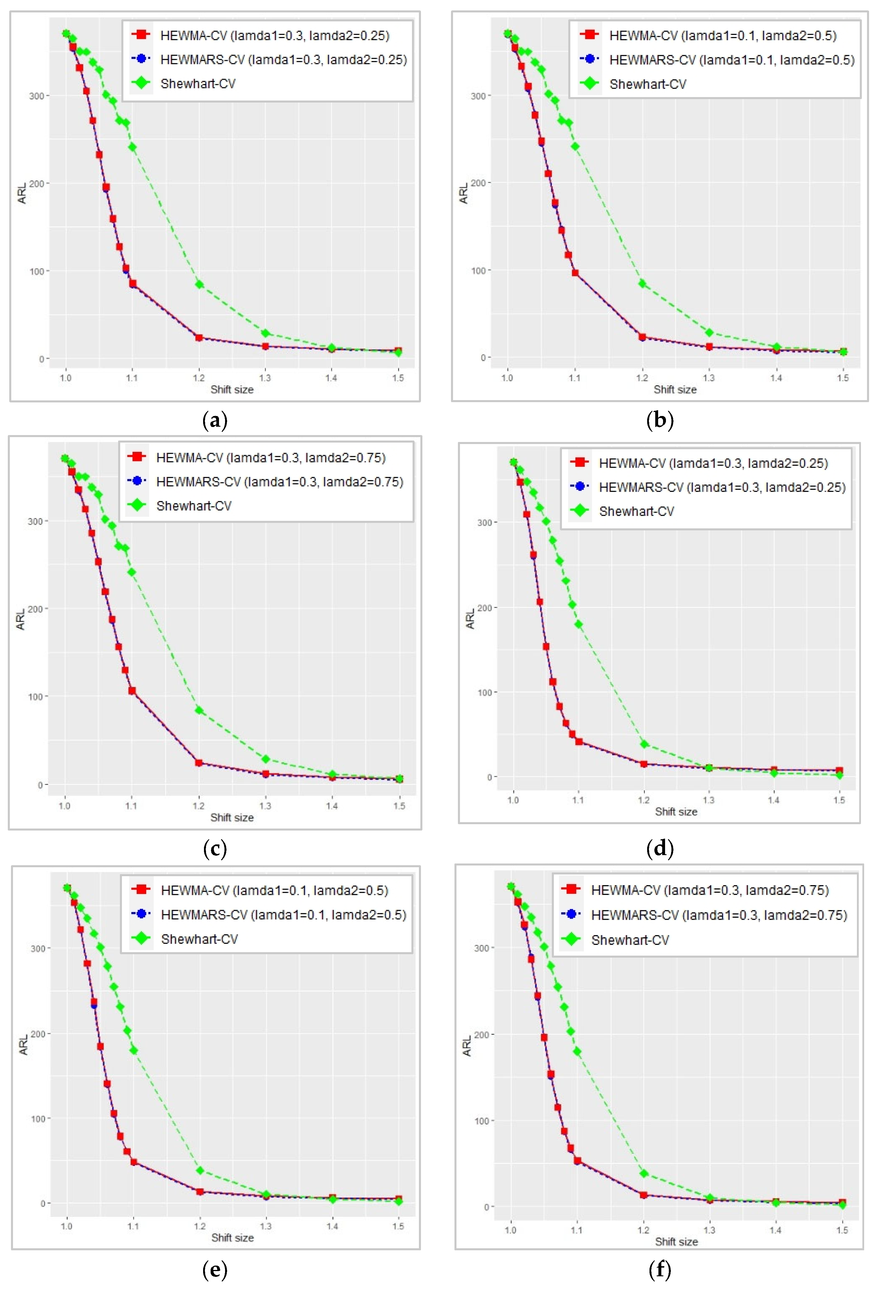
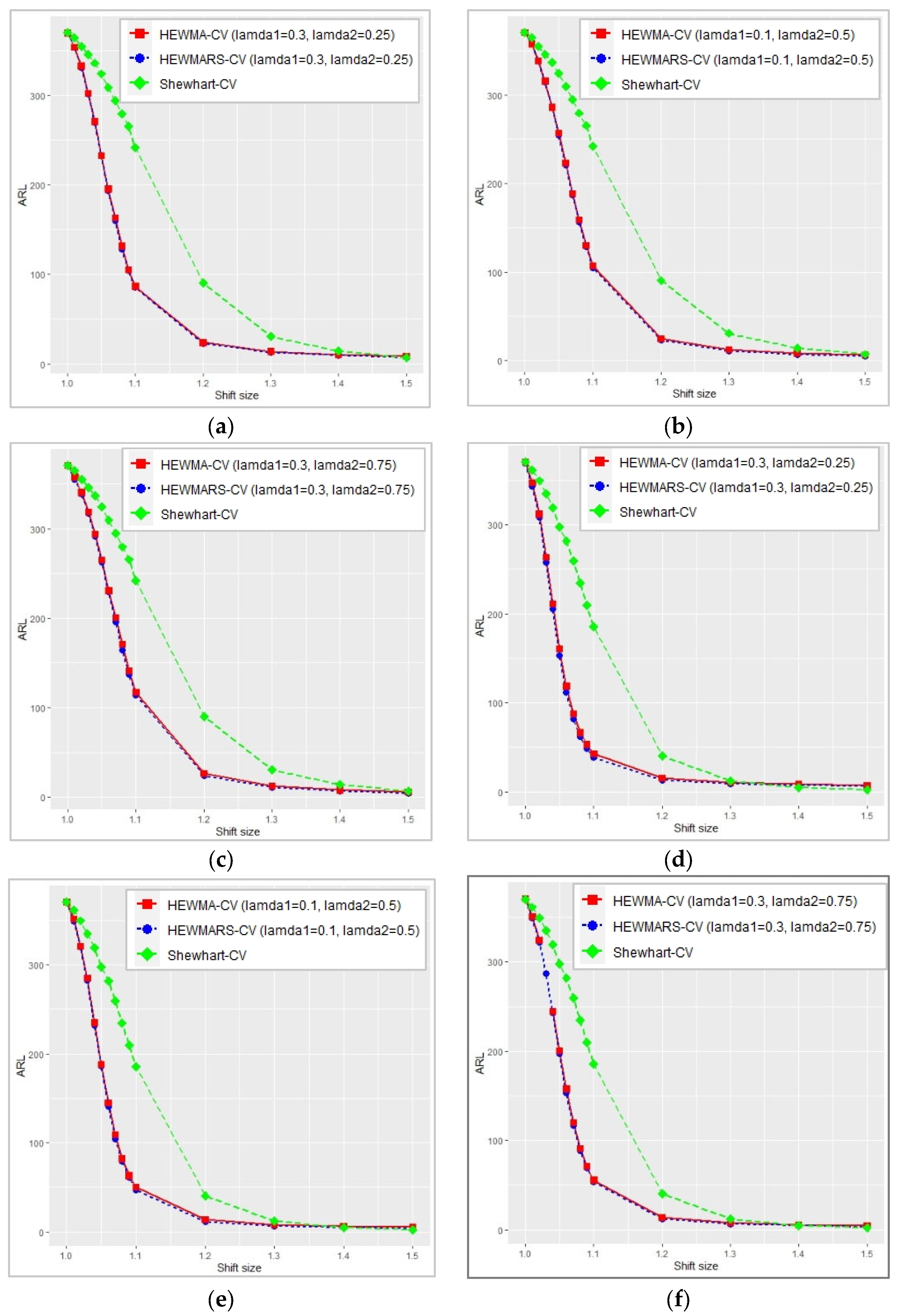
Figure 4.
Comparison of ARL between HEWMARS-CV, HEWMA-CV, and Shewhart Control Charts when the CV parameter = 0.10, the exponential smoothing parameter and various values of and the sample size is. (a) and n = 10; (b) and n = 10; (c) and n = 10; (d) and n = 20; (e) and n = 20; (f) and n = 20.
Figure 4.
Comparison of ARL between HEWMARS-CV, HEWMA-CV, and Shewhart Control Charts when the CV parameter = 0.10, the exponential smoothing parameter and various values of and the sample size is. (a) and n = 10; (b) and n = 10; (c) and n = 10; (d) and n = 20; (e) and n = 20; (f) and n = 20.
Figure 5.
Comparison of ARL between HEWMARS-CV, HEWMA-CV, and Shewhart Control Charts when the CV parameter = 0.15, the exponential smoothing parameter and various values of and the sample size is. (a) and n = 10; (b) and n = 10; (c) and n = 10; (d) and n = 20; (e) and n = 20; (f) and n = 20.
Figure 5.
Comparison of ARL between HEWMARS-CV, HEWMA-CV, and Shewhart Control Charts when the CV parameter = 0.15, the exponential smoothing parameter and various values of and the sample size is. (a) and n = 10; (b) and n = 10; (c) and n = 10; (d) and n = 20; (e) and n = 20; (f) and n = 20.
Figure 6.
Comparison of ARL between HEWMARS-CV, HEWMA-CV, and Shewhart Control Charts when the CV parameter = 0.15, the exponential smoothing parameter and various values of and the sample size is. (a) and n = 10; (b) and n = 10; (c) and n = 10; (d) and n = 20; (e) and n = 20; (f) and n = 20.
Figure 6.
Comparison of ARL between HEWMARS-CV, HEWMA-CV, and Shewhart Control Charts when the CV parameter = 0.15, the exponential smoothing parameter and various values of and the sample size is. (a) and n = 10; (b) and n = 10; (c) and n = 10; (d) and n = 20; (e) and n = 20; (f) and n = 20.
Figure 7.
Comparison of ARL between HEWMARS-CV, HEWMA-CV, and Shewhart Control Charts when the CV parameter = 0.20, the exponential smoothing parameter and various values of and the sample size is. (a) and n = 10; (b) and n = 10; (c) and n = 10; (d) and n = 20; (e) and n = 20; (f) and n = 20.
Figure 7.
Comparison of ARL between HEWMARS-CV, HEWMA-CV, and Shewhart Control Charts when the CV parameter = 0.20, the exponential smoothing parameter and various values of and the sample size is. (a) and n = 10; (b) and n = 10; (c) and n = 10; (d) and n = 20; (e) and n = 20; (f) and n = 20.
Figure 8.
Comparison of ARL between HEWMARS-CV, HEWMA-CV, and Shewhart Control Charts when the CV parameter = 0.20, the exponential smoothing parameter and various values of and the sample size is. (a) and n = 10; (b) and n = 10; (c) and n = 10; (d) and n = 20; (e) and n = 20; (f) and n = 20.
Figure 8.
Comparison of ARL between HEWMARS-CV, HEWMA-CV, and Shewhart Control Charts when the CV parameter = 0.20, the exponential smoothing parameter and various values of and the sample size is. (a) and n = 10; (b) and n = 10; (c) and n = 10; (d) and n = 20; (e) and n = 20; (f) and n = 20.
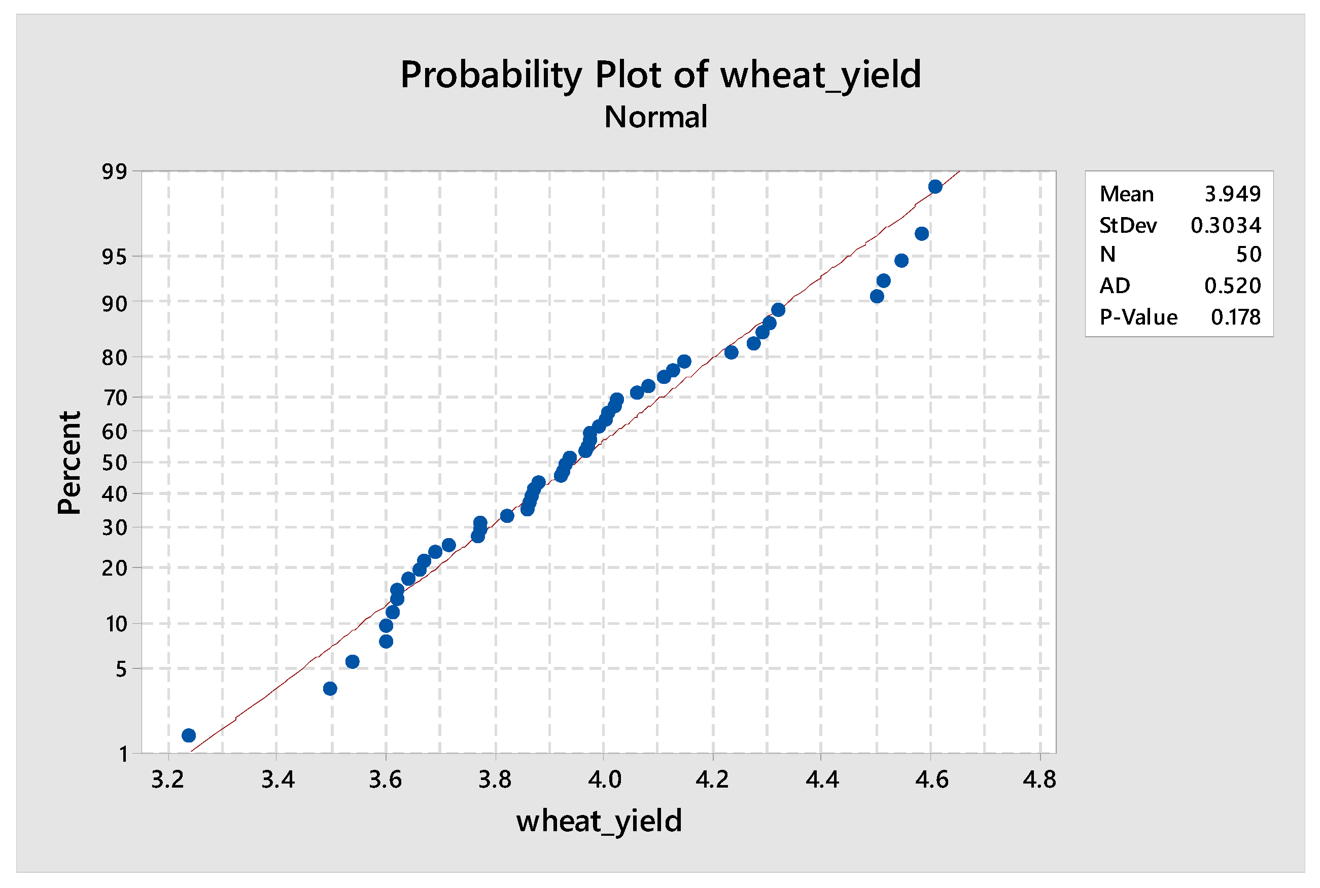
Figure 9.
The probability plot of wheat yield based on the Anderson–Darling test.
Figure 9.
The probability plot of wheat yield based on the Anderson–Darling test.
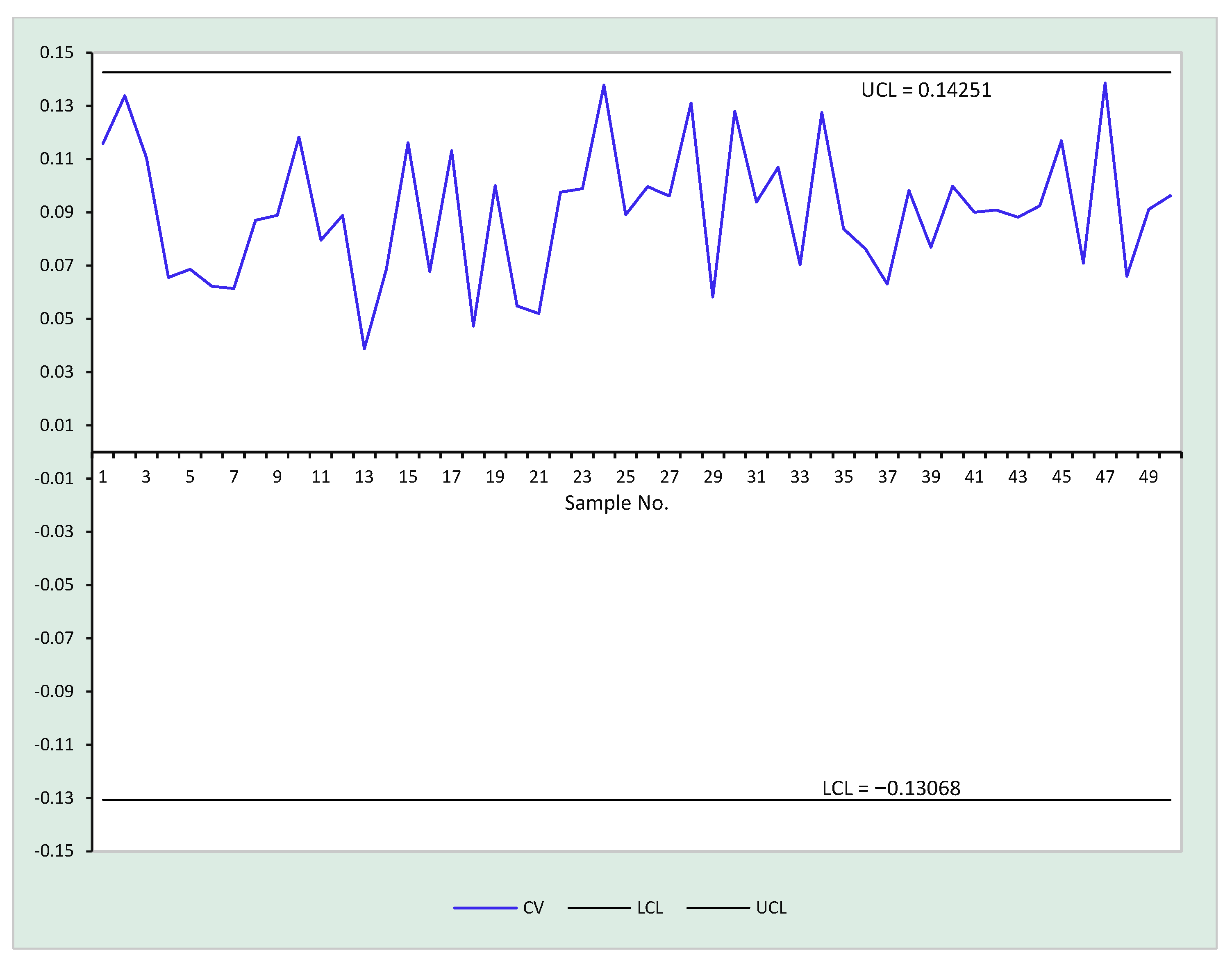
Figure 10.
Shewhart control chart with = 0.08 and n = 10.
Figure 10.
Shewhart control chart with = 0.08 and n = 10.
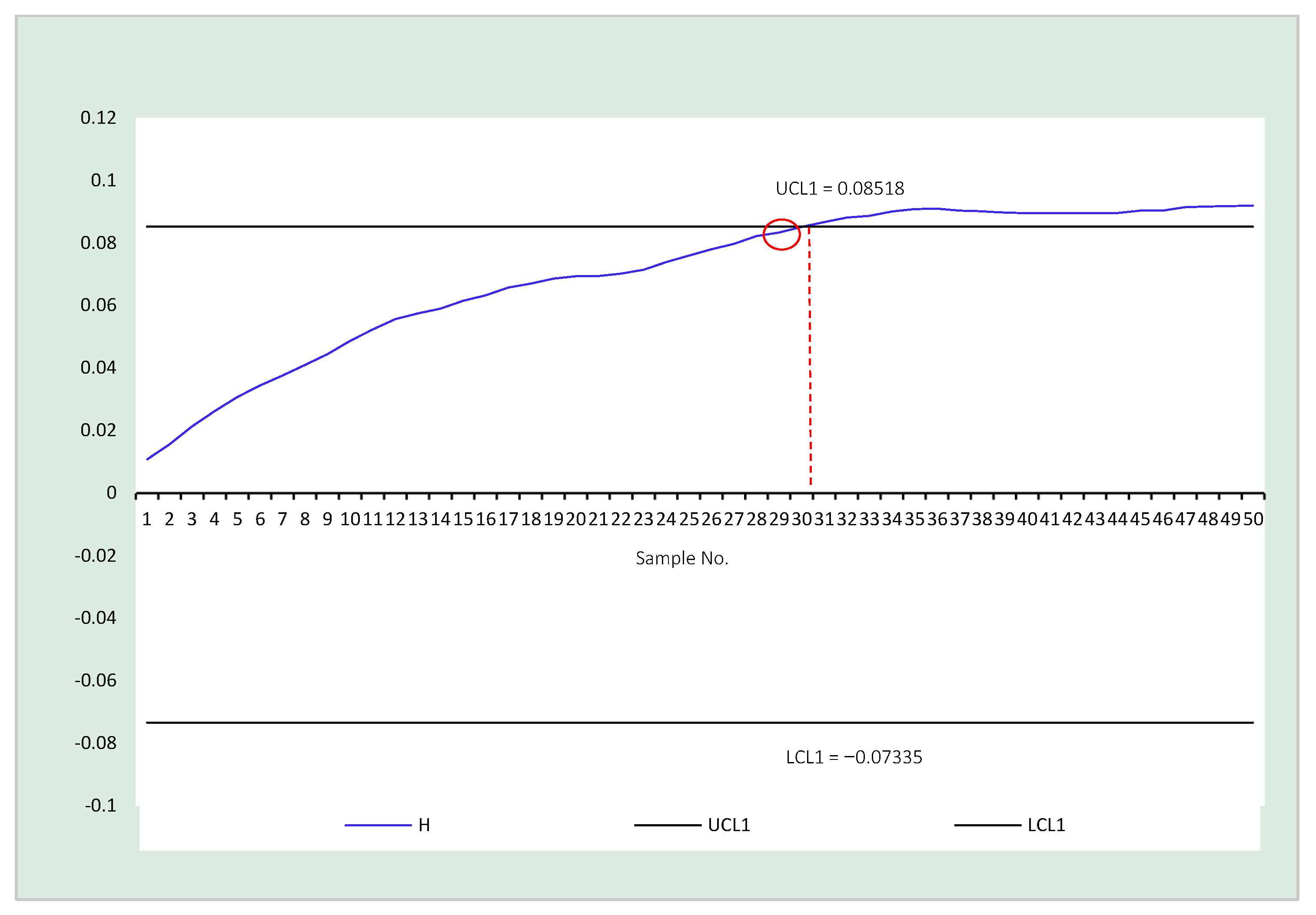
Figure 11.
HEWMA-CV control chart with = 0.08, = 0.10, = 0.25, and n = 10.
Figure 11.
HEWMA-CV control chart with = 0.08, = 0.10, = 0.25, and n = 10.
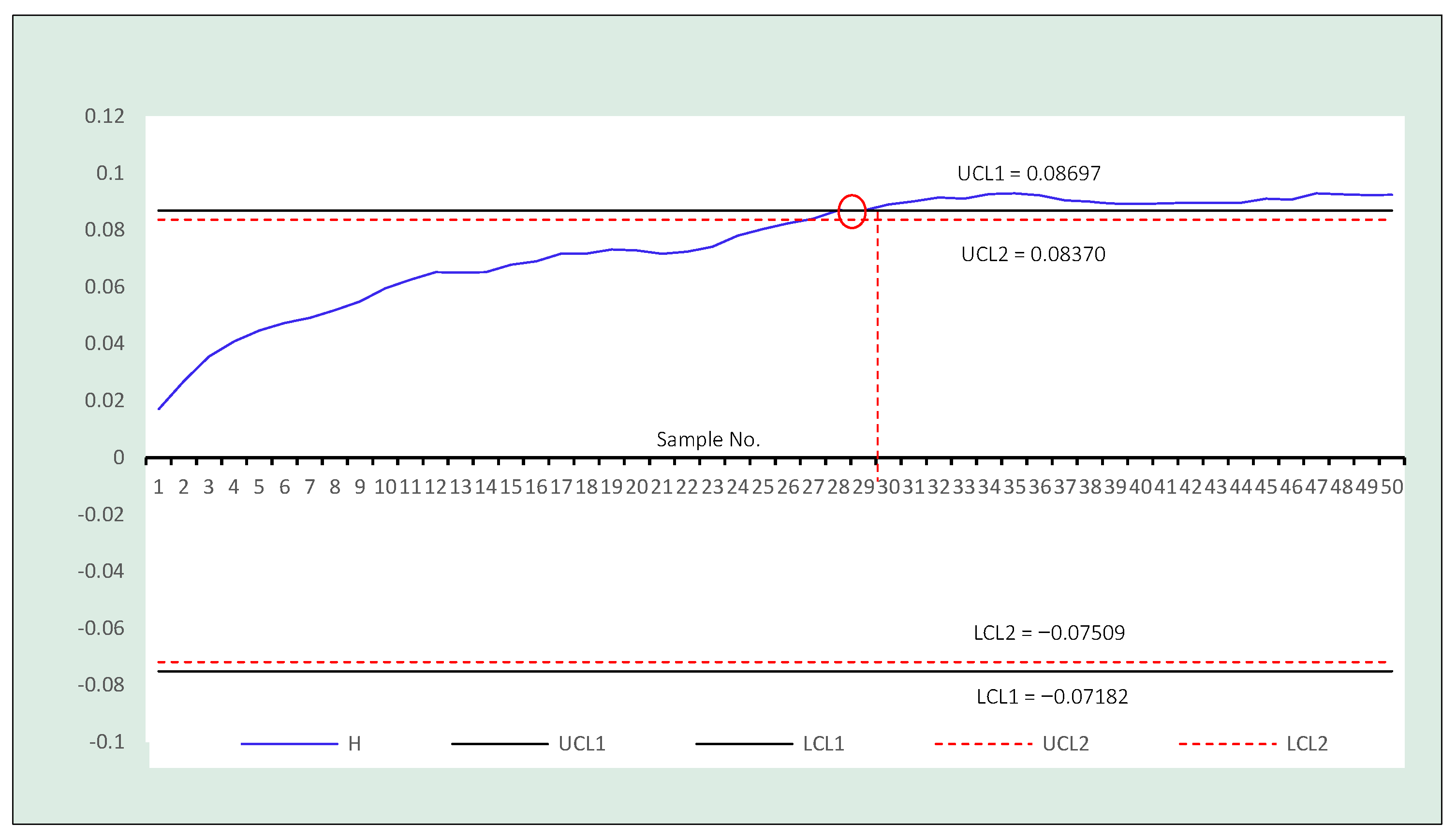
Figure 12.
HEWMARS-CV control chart with = 0.08, = 0.10, = 0.50, and n = 10.
Figure 12.
HEWMARS-CV control chart with = 0.08, = 0.10, = 0.50, and n = 10.
Table 1.
Comparison of ARL between HEWMARS-CV, HEWMA-CV, and Shewhart Control Charts given = 0.08 and = 0.10.
Table 1.
Comparison of ARL between HEWMARS-CV, HEWMA-CV, and Shewhart Control Charts given = 0.08 and = 0.10.
Sample Size
| Shift Size
| | HEWMARS-CV | | HEWMA-CV | | Shewhart-CV |
|---|
| 0.10, 0.25 | 0.10, 0.50 | 0.10, 0.75 | | 0.10, 0.25 | 0.10, 0.50 | 0.10, 0.75 | | |
|---|
| L1, L2 | 3.720, 3.610 | 2.480, 2.380 | 1.864, 1.856 | L | 3.710 | 2.475 | 1.863 | L | 2.250 |
|---|
| 10 | 1.00 | | 370.994 | 369.019 | 370.302 | | 370.991 | 370.177 | 370.556 | | 370.312 |
| | 1.01 | | 349.203 | 348.099 | 349.962 | | 351.132 | 352.090 | 352.563 | | 363.059 |
| | 1.02 | | 319.118 | 319.004 | 321.177 | | 320.636 | 323.997 | 325.174 | | 357.059 |
| | 1.03 | | 279.586 | 280.171 | 284.137 | | 284.292 | 285.769 | 286.929 | | 344.108 |
| | 1.04 | | 236.516 | 236.193 | 241.173 | | 238.384 | 244.117 | 246.208 | | 334.108 |
| | 1.05 | | 191.323 | 191.974 | 198.990 | | 196.195 | 202.736 | 203.088 | | 322.072 |
| | 1.06 | | 151.740 | 153.921 | 162.192 | | 157.733 | 163.493 | 165.504 | | 308.733 |
| | 1.07 | | 111.450 | 120.433 | 130.226 | | 125.891 | 131.115 | 131.841 | | 293.250 |
| | 1.08 | | 95.342 | 97.053 | 105.904 | | 101.038 | 106.680 | 107.446 | | 277.034 |
| | 1.09 | | 78.854 | 79.613 | 87.013 | | 85.861 | 88.841 | 89.597 | | 258.553 |
| | 1.10 | | 66.110 | 66.427 | 73.602 | | 72.958 | 75.735 | 75.626 | | 240.411 |
| | 1.20 | | 28.157 | 26.241 | 29.950 | | 32.373 | 31.361 | 31.213 | | 82.531 |
| | 1.30 | | 20.193 | 18.233 | 19.963 | | 23.069 | 21.534 | 21.248 | | 27.921 |
| | 1.40 | | 16.718 | 14.499 | 15.470 | | 16.732 | 17.067 | 16.648 | | 12.193 |
| | 1.50 | | 14.524 | 12.210 | 12.716 | | 14.560 | 14.349 | 13.868 | | 6.175 |
| | | | 0.10, 0.25 | 0.10, 0.50 | 0.10, 0.75 | | 0.10, 0.25 | 0.10, 0.50 | 0.10, 0.75 | | |
| | | L1, L2 | 4.540, 4.525 | 3.013, 2.980 | 2.261, 2.252 | L | 4.538 | 3.010 | 2.260 | L | 3.010 |
| 20 | 1.00 | | 369.917 | 370.134 | 369.228 | | 370.380 | 370.416 | 370.183 | | 370.559 |
| | 1.01 | | 335.234 | 335.390 | 337.395 | | 337.579 | 337.221 | 341.432 | | 361.402 |
| | 1.02 | | 281.225 | 286.748 | 287.063 | | 284.771 | 289.990 | 291.113 | | 350.244 |
| | 1.03 | | 218.747 | 224.371 | 229.707 | | 223.970 | 227.949 | 230.909 | | 334.545 |
| | 1.04 | | 159.266 | 166.920 | 169.223 | | 164.240 | 169.834 | 174.310 | | 318.723 |
| | 1.05 | | 115.123 | 121.949 | 124.246 | | 119.990 | 125.432 | 126.821 | | 300.025 |
| | 1.06 | | 89.220 | 90.840 | 94.002 | | 91.570 | 94.550 | 96.280 | | 279.018 |
| | 1.07 | | 71.246 | 71.650 | 74.330 | | 72.296 | 75.853 | 76.404 | | 253.826 |
| | 1.08 | | 59.205 | 59.207 | 61.097 | | 61.066 | 62.245 | 62.514 | | 229.839 |
| | 1.09 | | 50.533 | 50.764 | 51.850 | | 53.201 | 53.337 | 54.210 | | 201.499 |
| | 1.10 | | 45.592 | 44.450 | 45.736 | | 47.346 | 47.359 | 47.461 | | 178.254 |
| | 1.20 | | 24.800 | 22.699 | 23.015 | | 26.211 | 24.673 | 24.413 | | 36.586 |
| | 1.30 | | 19.104 | 16.765 | 16.674 | | 20.309 | 18.289 | 17.908 | | 10.604 |
| | 1.40 | | 16.024 | 13.646 | 13.348 | | 17.161 | 14.991 | 14.480 | | 4.097 |
| | 1.50 | | 13.999 | 11.591 | 11.198 | | 15.056 | 12.871 | 12.309 | | 1.952 |
Table 2.
Comparison of ARL between HEWMARS-CV, HEWMA-CV, and Shewhart Control Charts given = 0.08 and = 0.30.
Table 2.
Comparison of ARL between HEWMARS-CV, HEWMA-CV, and Shewhart Control Charts given = 0.08 and = 0.30.
Sample Size
| Shift Size
| | HEWMARS-CV | | HEWMA-CV | | Shewhart-CV |
|---|
| 0.30, 0.25 | 0.30, 0.50 | 0.30, 0.75 | | 0.30, 0.25 | 0.30, 0.50 | 0.30, 0.75 | | |
|---|
| L1, L2 | 2.182, 2.176 | 1.520, 1.380 | 1.162, 1.145 | L | 2.181 | 1.510 | 1.161 | L | 2.250 |
|---|
| 10 | 1.00 | | 370.363 | 370.231 | 369.983 | | 370.317 | 370.220 | 370.164 | | 370.312 |
| | 1.01 | | 352.514 | 354.319 | 355.298 | | 354.914 | 357.861 | 357.116 | | 363.059 |
| | 1.02 | | 330.883 | 335.231 | 337.604 | | 332.620 | 338.231 | 339.202 | | 357.059 |
| | 1.03 | | 300.883 | 310.835 | 314.751 | | 301.988 | 314.669 | 317.548 | | 344.108 |
| | 1.04 | | 263.935 | 279.657 | 287.332 | | 269.491 | 285.713 | 288.795 | | 334.108 |
| | 1.05 | | 227.352 | 245.563 | 254.964 | | 229.351 | 252.176 | 258.841 | | 322.072 |
| | 1.06 | | 189.591 | 213.415 | 222.439 | | 193.256 | 217.097 | 226.381 | | 308.733 |
| | 1.07 | | 155.338 | 174.930 | 188.732 | | 157.704 | 182.044 | 191.976 | | 293.250 |
| | 1.08 | | 122.831 | 143.953 | 152.690 | | 126.573 | 151.933 | 160.047 | | 277.034 |
| | 1.09 | | 99.167 | 115.200 | 130.988 | | 102.607 | 124.754 | 133.145 | | 258.553 |
| | 1.10 | | 81.126 | 94.765 | 107.595 | | 82.685 | 101.189 | 109.093 | | 240.411 |
| | 1.20 | | 22.126 | 19.356 | 23.395 | | 23.371 | 23.752 | 25.029 | | 82.531 |
| | 1.30 | | 12.802 | 9.356 | 10.688 | | 13.850 | 12.123 | 12.120 | | 27.921 |
| | 1.40 | | 9.408 | 6.250 | 6.782 | | 10.509 | 8.385 | 8.057 | | 12.193 |
| | 1.50 | | 7.675 | 4.816 | 4.889 | | 8.753 | 6.601 | 6.093 | | 6.175 |
| | | , | 0.30, 0.25 | 0.30, 0.50 | 0.30, 0.75 | , | 0.30, 0.25 | 0.30, 0.50 | 0.30, 0.75 | | |
| | | L1, L2 | 2.614, 2.599 | 1.780, 1.735 | 1.359, 1.328 | L | 2.615 | 1.779 | 1.357 | L | 3.010 |
| 20 | 1.00 | | 370.273 | 370.037 | 370.537 | | 370.280 | 370.220 | 370.182 | | 370.559 |
| | 1.01 | | 343.600 | 346.823 | 350.590 | | 344.693 | 350.905 | 351.129 | | 361.402 |
| | 1.02 | | 305.053 | 315.028 | 322.309 | | 307.042 | 319.436 | 323.073 | | 350.244 |
| | 1.03 | | 256.331 | 274.119 | 281.928 | | 258.696 | 275.761 | 283.931 | | 334.545 |
| | 1.04 | | 200.059 | 222.608 | 235.847 | | 203.737 | 231.874 | 239.278 | | 318.723 |
| | 1.05 | | 148.417 | 173.169 | 189.600 | | 151.400 | 180.052 | 191.684 | | 300.025 |
| | 1.06 | | 108.814 | 130.294 | 146.280 | | 111.570 | 153.955 | 148.480 | | 279.018 |
| | 1.07 | | 79.853 | 97.215 | 111.121 | | 82.554 | 100.780 | 109.926 | | 253.826 |
| | 1.08 | | 61.347 | 71.228 | 81.451 | | 62.870 | 76.306 | 83.446 | | 229.839 |
| | 1.09 | | 48.376 | 55.093 | 62.865 | | 50.000 | 59.191 | 64.716 | | 201.499 |
| | 1.10 | | 39.601 | 43.340 | 48.965 | | 41.197 | 47.034 | 50.886 | | 178.254 |
| | 1.20 | | 13.392 | 11.057 | 11.473 | | 15.265 | 13.376 | 13.330 | | 36.586 |
| | 1.30 | | 9.483 | 6.539 | 6.265 | | 10.686 | 8.237 | 7.799 | | 10.604 |
| | 1.40 | | 7.631 | 4.932 | 4.347 | | 8.765 | 6.300 | 5.799 | | 4.097 |
| | 1.50 | | 6.501 | 3.984 | 3.349 | | 7.583 | 5.300 | 4.600 | | 1.952 |
Table 3.
Comparison of ARL between HEWMARS-CV, HEWMA-CV and Shewhart Control Charts given = 0.10 and = 0.10.
Table 3.
Comparison of ARL between HEWMARS-CV, HEWMA-CV and Shewhart Control Charts given = 0.10 and = 0.10.
Sample Size
| Shift Size
| | HEWMARS-CV | | HEWMA-CV | | Shewhart-CV |
|---|
| 0.10, 0.25 | 0.10, 0.50 | 0.10, 0.75 | | 0.10, 0.25 | 0.10, 0.50 | 0.10, 0.75 | | |
|---|
| L1, L2 | 4.135, 4.128 | 2.761, 2.755 | 2.083, 2.005 | L | 4.135 | 2.761 | 2.083 | L | 2.235 |
|---|
| 10 | 1.00 | | 370.278 | 370.464 | 370.165 | | 370.063 | 370.200 | 370.447 | | 370.723 |
| | 1.01 | | 348.824 | 347.351 | 350.407 | | 350.246 | 350.083 | 353.997 | | 364.989 |
| | 1.02 | | 310.543 | 320.099 | 323.986 | | 319.047 | 319.591 | 325.724 | | 350.007 |
| | 1.03 | | 283.373 | 285.794 | 286.788 | | 283.706 | 283.867 | 289.888 | | 349.744 |
| | 1.04 | | 236.498 | 240.937 | 245.799 | | 242.375 | 243.282 | 252.391 | | 337.979 |
| | 1.05 | | 193.459 | 200.707 | 200.566 | | 197.920 | 199.265 | 210.185 | | 329.297 |
| | 1.06 | | 153.477 | 159.972 | 161.105 | | 156.970 | 162.178 | 169.872 | | 301.211 |
| | 1.07 | | 125.808 | 128.045 | 127.575 | | 125.848 | 131.082 | 137.465 | | 293.936 |
| | 1.08 | | 101.101 | 103.692 | 102.882 | | 103.256 | 105.889 | 111.346 | | 271.031 |
| | 1.09 | | 82.626 | 86.627 | 83.911 | | 85.805 | 87.224 | 91.431 | | 268.908 |
| | 1.10 | | 70.929 | 73.016 | 69.760 | | 72.285 | 74.998 | 78.038 | | 241.279 |
| | 1.20 | | 30.747 | 29.994 | 27.191 | | 31.821 | 31.426 | 31.289 | | 84.285 |
| | 1.30 | | 21.732 | 20.239 | 18.047 | | 22.837 | 21.371 | 21.146 | | 28.330 |
| | 1.40 | | 17.608 | 15.819 | 14.150 | | 18.668 | 16.916 | 16.529 | | 11.728 |
| | 1.50 | | 15.103 | 13.163 | 11.714 | | 16.132 | 14.188 | 13.764 | | 6.407 |
| | | , | 0.10, 0.25 | 0.10, 0.50 | 0.10, 0.75 | , | 0.10, 0.25 | 0.10, 0.50 | 0.10, 0.75 | | |
| | | L1, L2 | 5.071, 5.054 | 3.368, 3.355 | 2.527, 2.515 | L | 5.071 | 3.368 | 2.527 | L | 2.990 |
| 20 | 1.00 | | 370.197 | 370.845 | 370.167 | | 370.560 | 370.698 | 370.441 | | 370.870 |
| | 1.01 | | 336.136 | 343.096 | 337.367 | | 340.285 | 341.867 | 338.217 | | 362.121 |
| | 1.02 | | 289.520 | 293.128 | 289.735 | | 289.818 | 292.878 | 289.679 | | 347.938 |
| | 1.03 | | 221.018 | 229.114 | 230.158 | | 226.589 | 234.234 | 232.322 | | 335.171 |
| | 1.04 | | 159.216 | 172.399 | 172.955 | | 172.190 | 175.273 | 172.235 | | 317.302 |
| | 1.05 | | 116.324 | 126.402 | 125.512 | | 116.823 | 128.533 | 127.572 | | 300.914 |
| | 1.06 | | 89.724 | 95.107 | 95.082 | | 90.220 | 96.813 | 96.332 | | 278.986 |
| | 1.07 | | 71.078 | 75.467 | 74.596 | | 71.780 | 76.400 | 76.341 | | 254.704 |
| | 1.08 | | 60.759 | 61.493 | 61.460 | | 61.224 | 63.665 | 63.073 | | 230.906 |
| | 1.09 | | 50.761 | 52.491 | 52.725 | | 53.138 | 53.852 | 54.085 | | 202.941 |
| | 1.10 | | 45.432 | 45.940 | 45.886 | | 47.095 | 47.272 | 47.333 | | 179.432 |
| | 1.20 | | 24.724 | 23.234 | 22.853 | | 25.988 | 24.612 | 24.318 | | 38.258 |
| | 1.30 | | 18.963 | 17.019 | 16.513 | | 20.115 | 18.182 | 17.683 | | 10.524 |
| | 1.40 | | 15.882 | 13.763 | 13.194 | | 16.986 | 14.863 | 14.337 | | 4.194 |
| | 1.50 | | 13.847 | 11.634 | 11.037 | | 14.929 | 12.715 | 12.148 | | 1.994 |
Table 4.
Comparison of ARL between HEWMARS-CV, HEWMA-CV, and Shewhart Control Charts given = 0.10 and = 0.30.
Table 4.
Comparison of ARL between HEWMARS-CV, HEWMA-CV, and Shewhart Control Charts given = 0.10 and = 0.30.
Sample Size
n | Shift Size
| | HEWMARS-CV | | HEWMA-CV | | Shewhart-CV |
|---|
| 0.30, 0.25 | 0.30, 0.50 | 0.30, 0.75 | | 0.30, 0.25 | 0.30, 0.50 | 0.30, 0.75 | | |
|---|
| L1, L2 | 2.439, 2.430 | 1.685,1.675 | 1.299, 1.290 | L | 2.439 | 1.685 | 1.299 | L | 2.235 |
|---|
| 10 | 1.00 | | 369.648 | 369.256 | 370.715 | | 370.593 | 370.623 | 370.731 | | 370.723 |
| | 1.01 | | 353.636 | 352.458 | 355.372 | | 355.554 | 354.739 | 355.449 | | 364.989 |
| | 1.02 | | 331.934 | 332.597 | 333.755 | |
331.797
| 333.286 | 335.516 | | 350.007 |
| | 1.03 | | 305.946 | 306.991 | 312.821 | | 305.010 | 310.372 | 313.069 | | 349.744 |
| | 1.04 | | 270.623 | 278.384 | 284.826 | |
271.365
| 277.306 | 285.781 | | 337.979 |
| | 1.05 | | 233.991 | 244.647 | 254.175 | | 232.533 | 247.734 | 253.182 | | 329.297 |
| | 1.06 | | 192.880 | 211.190 | 219.484 | | 195.327 | 210.317 | 219.095 | | 301.211 |
| | 1.07 | | 157.989 | 173.904 | 186.266 | | 159.377 | 177.044 | 187.690 | | 293.936 |
| | 1.08 | | 127.449 | 146.665 | 157.316 | | 127.221 | 145.067 | 156.370 | | 271.031 |
| | 1.09 | | 100.216 | 116.932 | 129.884 | | 103.301 | 117.278 | 130.089 | | 268.908 |
| | 1.10 | | 83.675 | 96.604 | 105.434 | | 85.294 | 96.568 | 106.599 | | 241.279 |
| | 1.20 | | 22.427 | 22.049 | 23.369 | | 23.414 | 23.101 | 24.445 | | 84.285 |
| | 1.30 | | 12.753 | 10.864 | 10.835 | | 13.852 | 12.088 | 11.962 | | 28.330 |
| | 1.40 | | 9.370 | 7.146 | 6.910 | | 10.426 | 8.336 | 7.964 | | 11.728 |
| | 1.50 | | 7.634 | 5.419 | 4.949 | | 8.693 | 6.536 | 6.027 | | 6.407 |
| | | , | 0.30, 0.25 | 0.30, 0.50 | 0.30, 0.75 | , | 0.30, 0.25 | 0.30, 0.50 | 0.30, 0.75 | | |
| | | L1, L2 | 2.925, 2.915 | 1.995, 1.990 | 1.523, 1.518 | L | 2.925 | 1.995 | 1.523 | L | 2.990 |
| 20 | 1.00 | | 370.812 | 370.917 | 370.209 | | 370.983 | 370.984 | 370.755 | | 370.870 |
| | 1.01 | | 347.666 | 353.638 | 351.636 | | 347.386 | 353.316 | 352.912 | | 362.121 |
| | 1.02 | | 308.833 | 320.910 | 323.733 | | 309.324 | 321.929 | 326.688 | | 347.938 |
| | 1.03 | | 259.886 | 281.868 | 289.519 | | 261.934 | 282.110 | 286.469 | | 335.171 |
| | 1.04 | | 205.754 | 231.844 | 242.173 | | 206.590 | 237.014 | 244.398 | | 317.302 |
| | 1.05 | | 153.682 | 183.443 | 196.377 | | 153.401 | 184.270 | 195.778 | | 300.914 |
| | 1.06 | | 111.950 | 138.644 | 150.663 | | 112.136 | 140.725 | 153.579 | | 278.986 |
| | 1.07 | | 82.363 | 104.081 | 115.662 | | 82.712 | 105.578 | 114.768 | | 254.704 |
| | 1.08 | | 62.171 | 77.229 | 86.938 | | 63.450 | 78.581 | 87.542 | | 230.906 |
| | 1.09 | | 49.560 | 60.524 | 65.853 | | 50.492 | 60.911 | 67.833 | | 202.941 |
| | 1.10 | | 40.607 | 47.215 | 51.674 | | 41.446 | 48.584 | 53.402 | | 179.432 |
| | 1.20 | | 14.001 | 12.248 | 12.355 | | 15.206 | 13.331 | 13.467 | | 38.258 |
| | 1.30 | | 9.551 | 7.137 | 6.710 | | 10.656 | 8.215 | 7.779 | | 10.524 |
| | 1.40 | | 7.630 | 5.248 | 4.625 | | 8.692 | 6.281 | 5.713 | | 4.194 |
| | 1.50 | | 6.504 | 4.208 | 3.537 | | 7.534 | 5.242 | 4.611 | | 1.994 |
Table 5.
Comparison of ARL between HEWMARS-CV, HEWMA-CV, and Shewhart Control Charts given = 0.15 and .
Table 5.
Comparison of ARL between HEWMARS-CV, HEWMA-CV, and Shewhart Control Charts given = 0.15 and .
Sample Size
| Shift Size
| | HEWMARS-CV | | HEWMA-CV | | Shewhart-CV |
|---|
| 0.10, 0.25 | 0.10, 0.50 | 0.10, 0.75 | | 0.10, 0.25 | 0.10, 0.50 | 0.10, 0.75 | | |
|---|
| L1, L2 | 4.836, 4.815 | 3.232, 3.100 | 2.436, 2.414 | L | 4.836 | 3.232 | 2.436 | L | 2.205 |
|---|
| 10 | 1.00 | | 370.046 | 370.545 | 370.153 | | 370.162 | 370.350 | 370.847 | | 370.713 |
| | 1.01 | | 348.798 | 343.668 | 350.031 | | 349.685 | 353.057 | 348.925 | | 363.408 |
| | 1.02 | | 319.560 | 320.606 | 323.024 | | 319.839 | 320.916 | 321.470 | | 357.367 |
| | 1.03 | | 280.270 | 267.917 | 284.861 | | 284.445 | 282.813 | 286.855 | | 46.168 |
| | 1.04 | | 236.534 | 226.970 | 246.092 | | 241.236 | 224.561 | 245.293 | | 332.012 |
| | 1.05 | | 195.943 | 191.432 | 204.007 | | 192.118 | 197.464 | 202.769 | | 322.639 |
| | 1.06 | | 156.444 | 149.176 | 164.483 | | 157.466 | 162.834 | 165.453 | | 309.205 |
| | 1.07 | | 123.021 | 113.573 | 131.744 | | 126.626 | 136.697 | 132.266 | | 294.718 |
| | 1.08 | | 101.456 | 99.414 | 107.056 | | 102.908 | 103.085 | 108.633 | | 277.690 |
| | 1.09 | | 84.886 | 77.493 | 88.320 | | 85.108 | 89.470 | 89.930 | | 262.326 |
| | 1.10 | | 71.666 | 74.213 | 74.349 | | 72.746 | 75.308 | 76.490 | | 243.924 |
| | 1.20 | | 30.281 | 29.923 | 29.396 | | 31.786 | 30.912 | 30.824 | | 85.366 |
| | 1.30 | | 21.340 | 20.049 | 19.314 | | 22.496 | 21.082 | 20.782 | | 29.431 |
| | 1.40 | | 17.176 | 15.540 | 14.783 | | 18.346 | 16.542 | 16.153 | | 13.003 |
| | 1.50 | | 14.687 | 12.858 | 12.148 | | 15.792 | 13.858 | 13.366 | | 6.750 |
| | | , | 0.10, 0.25 | 0.10, 0.50 | 0.10, 0.75 | , | 0.10, 0.25 | 0.10, 0.50 | 0.10, 0.75 | | |
| | | L1, L2 | 5.970, 5.869 | 3.961, 3.960 | 2.975, 2.965 | L | 5.970 | 3.961 | 2.975 | L | 2.975 |
| 20 | 1.00 | | 370.570 | 370.450 | 370.662 | | 370.267 | 370.479 | 370.083 | | 370.898 |
| | 1.01 | | 337.676 | 331.952 | 339.109 | | 343.264 | 337.476 | 339.767 | | 359.399 |
| | 1.02 | | 286.948 | 290.236 | 288.891 | | 291.885 | 290.350 | 290.265 | | 351.302 |
| | 1.03 | | 223.539 | 228.588 | 231.633 | | 232.813 | 238.003 | 231.110 | | 337.361 |
| | 1.04 | | 164.149 | 175.956 | 173.814 | | 172.635 | 175.987 | 174.802 | | 321.599 |
| | 1.05 | | 118.005 | 126.497 | 126.648 | | 125.258 | 131.618 | 129.807 | | 303.489 |
| | 1.06 | | 88.724 | 93.198 | 95.945 | | 94.793 | 95.837 | 97.743 | | 280.582 |
| | 1.07 | | 69.235 | 76.151 | 75.598 | | 75.616 | 76.229 | 77.291 | | 260.188 |
| | 1.08 | | 57.071 | 60.423 | 61.975 | | 63.098 | 61.554 | 64.155 | | 232.593 |
| | 1.09 | | 48.505 | 52.166 | 52.375 | | 53.741 | 53.127 | 53.822 | | 207.865 |
| | 1.10 | | 42.911 | 46.203 | 46.017 | | 47.827 | 47.201 | 47.617 | | 182.083 |
| | 1.20 | | 23.282 | 23.201 | 22.701 | | 25.740 | 24.176 | 23.921 | | 39.074 |
| | 1.30 | | 18.098 | 16.818 | 16.231 | | 19.807 | 17.823 | 17.386 | | 11.291 |
| | 1.40 | | 15.134 | 13.507 | 12.925 | | 16.654 | 14.511 | 13.990 | | 4.485 |
| | 1.50 | | 13.203 | 11.397 | 10.745 | | 14.617 | 12.395 | 11.845 | | 2.110 |
Table 6.
Comparison of ARL between HEWMARS-CV, HEWMA-CV, and Shewhart Control Charts given = 0.15 and .
Table 6.
Comparison of ARL between HEWMARS-CV, HEWMA-CV, and Shewhart Control Charts given = 0.15 and .
Sample Size
| Shift Size
| | HEWMARS-CV | | HEWMA-CV | | Shewhart-CV |
|---|
| 0.30, 0.25 | 0.30, 0.50 | 0.30, 0.75 | | 0.30, 0.25 | 0.30, 0.50 | 0.30, 0.75 | | |
|---|
| L1, L2 | 2.865, 2.850 | 1.990, 1.985 | 1.540, 1.535 | L | 2.865 | 1.990 | 1.540 | L | 2.205 |
|---|
| 10 | 1.00 | | 370.386 | 370.348 | 370.739 | | 369.830 | 369.791 | 370.002 | | 370.713 |
| | 1.01 | | 355.792 | 356.090 | 357.528 | | 354.528 | 356.020 | 360.141 | | 363.408 |
| | 1.02 | | 332.336 | 338.257 | 341.108 | | 334.573 | 337.650 | 342.545 | | 357.367 |
| | 1.03 | | 303.942 | 313.520 | 319.727 | | 305.077 | 312.645 | 320.574 | | 346.168 |
| | 1.04 | | 269.631 | 286.346 | 294.800 | | 270.487 | 286.861 | 294.578 | | 332.012 |
| | 1.05 | | 232.259 | 253.710 | 265.217 | | 231.954 | 252.959 | 266.166 | | 322.639 |
| | 1.06 | | 195.681 | 217.215 | 232.456 | | 197.013 | 219.712 | 231.389 | | 309.205 |
| | 1.07 | | 160.039 | 184.599 | 199.570 | | 161.697 | 184.066 | 202.138 | | 294.718 |
| | 1.08 | | 129.527 | 150.981 | 166.101 | | 129.012 | 151.575 | 169.833 | | 277.690 |
| | 1.09 | | 103.810 | 126.228 | 139.785 | | 103.810 | 127.694 | 138.965 | | 262.326 |
| | 1.10 | | 84.504 | 101.139 | 115.614 | | 86.463 | 104.953 | 115.540 | | 243.924 |
| | 1.20 | | 22.402 | 23.074 | 25.120 | | 23.723 | 24.101 | 26.159 | | 85.366 |
| | 1.30 | | 12.593 | 11.040 | 11.308 | | 13.660 | 12.238 | 12.308 | | 29.431 |
| | 1.40 | | 9.246 | 7.282 | 7.073 | | 10.290 | 8.309 | 8.058 | | 13.003 |
| | 1.50 | | 7.469 | 5.459 | 5.039 | | 8.562 | 6.528 | 6.074 | | 6.750 |
| | | , | 0.30, 0.25 | 0.30, 0.50 | 0.30, 0.75 | , | 0.30, 0.25 | 0.30, 0.50 | 0.30, 0.75 | | |
| | | L1, L2 | 3.450, 3.445 | 2.359, 2.350 | 1.805, 1.795 | L | 3.450 | 2.359 | 1.805 | L | 2.975 |
| 20 | 1.00 | | 370.161 | 370.487 | 369.534 | | 370.814 | 370.903 | 370.870 | | 370.898 |
| | 1.01 | | 345.069 | 352.521 | 351.638 | | 346.010 | 351.545 | 350.742 | | 359.399 |
| | 1.02 | | 310.309 | 322.531 | 326.772 | | 305.664 | 321.163 | 325.401 | | 351.302 |
| | 1.03 | | 259.106 | 278.847 | 289.351 | | 255.873 | 279.602 | 291.561 | | 337.361 |
| | 1.04 | | 205.310 | 230.498 | 244.575 | | 204.371 | 234.185 | 245.392 | | 321.599 |
| | 1.05 | | 153.714 | 185.322 | 199.188 | | 153.916 | 184.319 | 199.518 | | 303.489 |
| | 1.06 | | 113.636 | 140.684 | 153.304 | | 114.174 | 140.584 | 153.948 | | 280.582 |
| | 1.07 | | 84.657 | 106.091 | 116.334 | | 83.846 | 105.556 | 119.239 | | 260.188 |
| | 1.08 | | 63.672 | 78.576 | 87.823 | | 65.148 | 79.851 | 88.689 | | 232.593 |
| | 1.09 | | 50.176 | 60.390 | 67.639 | | 51.483 | 62.115 | 69.197 | | 207.865 |
| | 1.10 | | 40.930 | 46.677 | 53.278 | | 42.073 | 49.226 | 53.518 | | 182.083 |
| | 1.20 | | 14.104 | 12.305 | 12.469 | | 15.181 | 13.558 | 13.677 | | 39.074 |
| | 1.30 | | 9.514 | 7.054 | 6.647 | | 10.508 | 8.190 | 7.729 | | 11.291 |
| | 1.40 | | 7.548 | 5.117 | 4.538 | | 8.558 | 6.200 | 5.637 | | 4.485 |
| | 1.50 | | 6.387 | 4.105 | 3.448 | | 7.398 | 5.137 | 4.525 | | 2.110 |
Table 7.
Comparison of ARL between HEWMARS-CV, HEWMA-CV, and Shewhart Control Charts given = 0.20 and .
Table 7.
Comparison of ARL between HEWMARS-CV, HEWMA-CV, and Shewhart Control Charts given = 0.20 and .
Sample Size
| Shift Size
| | HEWMARS-CV | | HEWMA-CV | | Shewhart-CV |
|---|
| 0.10, 0.25 | 0.10, 0.50 | 0.10, 0.75 | | 0.10, 0.25 | 0.10, 0.50 | 0.10, 0.75 | | |
|---|
| L1, L2 | 5.331, 5.315 | 3.572, 3.549 | 2.695, 2.685 | L | 5.313 | 3.549 | 2.695 | L | 2.193 |
|---|
| 10 | 1.00 | | 370.545 | 370.237 | 370.191 | | 370.907 | 370.839 | 370.136 | | 370.364 |
| | 1.01 | | 351.120 | 353.490 | 351.682 | | 351.155 | 352.527 | 352.970 | | 364.558 |
| | 1.02 | | 320.144 | 323.914 | 324.892 | | 320.813 | 326.774 | 327.014 | | 354.944 |
| | 1.03 | | 281.777 | 289.968 | 290.934 | | 284.239 | 291.548 | 292.628 | | 345.996 |
| | 1.04 | | 241.023 | 249.953 | 252.208 | | 243.290 | 250.577 | 251.541 | | 336.386 |
| | 1.05 | | 196.591 | 209.215 | 208.220 | | 198.497 | 208.637 | 209.267 | | 324.123 |
| | 1.06 | | 158.713 | 166.244 | 171.646 | | 160.275 | 168.367 | 172.977 | | 309.150 |
| | 1.07 | | 126.770 | 134.381 | 137.548 | | 127.222 | 135.553 | 137.828 | | 294.483 |
| | 1.08 | | 103.745 | 111.001 | 112.472 | | 104.772 | 112.216 | 112.306 | | 279.421 |
| | 1.09 | | 86.291 | 90.121 | 91.052 | | 86.988 | 92.007 | 93.851 | | 265.427 |
| | 1.10 | | 72.282 | 76.427 | 77.627 | | 74.670 | 77.955 | 78.601 | | 242.006 |
| | 1.20 | | 30.399 | 29.533 | 29.837 | | 31.614 | 31.092 | 30.768 | | 90.228 |
| | 1.30 | | 21.045 | 19.543 | 19.451 | | 22.283 | 20.864 | 20.567 | | 30.948 |
| | 1.40 | | 16.883 | 15.058 | 14.720 | | 17.980 | 16.321 | 15.912 | | 13.989 |
| | 1.50 | | 14.396 | 12.399 | 12.009 | | 15.466 | 13.554 | 13.108 | | 7.147 |
| | | , | 0.10, 0.25 | 0.10, 0.50 | 0.10, 0.75 | , | 0.10, 0.25 | 0.10, 0.50 | 0.10, 0.75 | | |
| | | L1, L2 | 6.631, 6.610 | 4.412, 4.409 | 3.315, 3.310 | L | 6.631 | 4.412 | 3.315 | L | 2.993 |
| 20 | 1.00 | | 370.450 | 370.988 | 370.149 | | 370.445 | 370.838 | 370.518 | | 370.320 |
| | 1.01 | | 338.016 | 340.797 | 341.538 | | 338.446 | 342.438 | 341.757 | | 361.470 |
| | 1.02 | | 287.926 | 293.949 | 295.018 | | 289.641 | 294.954 | 295.341 | | 349.509 |
| | 1.03 | | 225.019 | 237.311 | 237.201 | | 225.536 | 237.820 | 237.415 | | 335.222 |
| | 1.04 | | 169.383 | 178.566 | 176.123 | | 169.387 | 179.550 | 179.566 | | 319.512 |
| | 1.05 | | 121.888 | 129.676 | 131.417 | | 122.824 | 131.112 | 132.322 | | 297.868 |
| | 1.06 | | 92.827 | 98.708 | 99.941 | | 93.875 | 99.761 | 100.188 | | 281.957 |
| | 1.07 | | 17.375 | 77.999 | 77.828 | | 74.489 | 78.051 | 78.584 | | 259.506 |
| | 1.08 | | 60.975 | 63.536 | 63.924 | | 62.288 | 63.979 | 64.934 | | 234.765 |
| | 1.09 | | 52.260 | 53.559 | 54.267 | | 53.412 | 55.077 | 55.047 | | 209.703 |
| | 1.10 | | 45.546 | 46.926 | 46.648 | | 47.112 | 47.687 | 47.664 | | 185.877 |
| | 1.20 | | 24.117 | 22.911 | 22.643 | | 25.409 | 23.995 | 23.787 | | 40.611 |
| | 1.30 | | 18.285 | 16.493 | 16.064 | | 19.362 | 17.505 | 17.133 | | 12.044 |
| | 1.40 | | 15.188 | 13.193 | 12.616 | | 16.280 | 14.148 | 13.658 | | 4.828 |
| | 1.50 | | 13.152 | 11.063 | 10.496 | | 14.248 | 12.078 | 11.533 | | 2.310 |
Table 8.
Comparison of ARL between HEWMARS-CV, HEWMA-CV, and Shewhart Control Charts given = 0.20 and .
Table 8.
Comparison of ARL between HEWMARS-CV, HEWMA-CV, and Shewhart Control Charts given = 0.20 and .
Sample Size
| Shift Size
| | HEWMARS-CV | | HEWMA-CV | | Shewhart-CV |
|---|
| 0.30, 0.25 | 0.30, 0.50 | 0.30, 0.75 | | 0.30, 0.25 | 0.30, 0.50 | 0.30, 0.75 | | |
|---|
| L1, L2 | 3.173, 3.150 | 2.216, 2.178 | 1.717, 1.651 | L | 3.174 | 2.217 | 1.718 | L | 2.193 |
|---|
| 10 | 1.00 | | 369.888 | 370.106 | 369.844 | | 370.081 | 370.328 | 370.542 | | 370.364 |
| | 1.01 | | 354.024 | 357.120 | 354.613 | | 354.065 | 357.693 | 357.696 | | 364.558 |
| | 1.02 | | 331.060 | 338.109 | 338.460 | | 332.974 | 338.192 | 340.402 | | 354.944 |
| | 1.03 | | 301.690 | 314.014 | 317.075 | | 302.577 | 315.615 | 318.377 | | 345.996 |
| | 1.04 | | 269.392 | 285.313 | 291.268 | | 271.081 | 286.036 | 293.641 | | 336.386 |
| | 1.05 | | 232.577 | 254.243 | 262.540 | | 232.854 | 256.705 | 264.752 | | 324.123 |
| | 1.06 | | 193.637 | 220.564 | 229.468 | | 195.599 | 223.257 | 230.882 | | 309.150 |
| | 1.07 | | 160.236 | 187.136 | 195.996 | | 163.451 | 188.461 | 200.638 | | 294.483 |
| | 1.08 | | 128.366 | 156.156 | 164.734 | | 131.679 | 158.972 | 170.754 | | 279.421 |
| | 1.09 | | 104.742 | 128.579 | 137.372 | | 105.330 | 130.209 | 141.365 | | 265.427 |
| | 1.10 | | 85.590 | 104.907 | 114.052 | | 86.690 | 107.103 | 117.122 | | 242.006 |
| | 1.20 | | 22.652 | 23.313 | 23.826 | | 23.793 | 25.010 | 26.577 | | 90.228 |
| | 1.30 | | 12.572 | 10.925 | 10.683 | | 13.822 | 12.430 | 12.471 | | 30.948 |
| | 1.40 | | 9.116 | 7.051 | 6.449 | | 10.267 | 8.375 | 8.105 | | 13.989 |
| | 1.50 | | 7.294 | 5.257 | 4.564 | | 8.467 | 6.491 | 6.032 | | 7.147 |
| | | , | 0.30, 0.25 | 0.30, 0.50 | 0.30, 0.75 | , | 0.30, 0.25 | 0.30, 0.50 | 0.30, 0.75 | | |
| | | L1, L2 | 3.853, 3.760 | 2.643, 2.560 | 2.024, 1.998 | L | 3.854 | 2.642 | 2.025 | L | 2.993 |
| 20 | 1.00 | | 369.120 | 370.126 | 370.463 | | 370.667 | 370.652 | 370.998 | | 370.320 |
| | 1.01 | | 342.961 | 349.165 | 349.617 | | 347.327 | 351.445 | 351.120 | | 361.470 |
| | 1.02 | | 308.384 | 320.179 | 322.054 | | 312.222 | 321.054 | 324.679 | | 349.509 |
| | 1.03 | | 258.112 | 282.322 | 286.754 | | 263.606 | 284.962 | 288.170 | | 335.222 |
| | 1.04 | | 205.205 | 231.788 | 243.416 | | 211.288 | 234.969 | 244.768 | | 319.512 |
| | 1.05 | | 153.314 | 186.083 | 197.054 | | 160.725 | 188.138 | 200.732 | | 297.868 |
| | 1.06 | | 111.566 | 140.980 | 152.938 | | 118.708 | 144.740 | 157.965 | | 281.957 |
| | 1.07 | | 81.791 | 104.430 | 116.809 | | 87.839 | 109.048 | 119.888 | | 259.506 |
| | 1.08 | | 62.282 | 78.920 | 88.256 | | 66.596 | 82.266 | 91.243 | | 234.765 |
| | 1.09 | | 48.416 | 60.693 | 69.160 | | 53.240 | 63.168 | 70.891 | | 209.703 |
| | 1.10 | | 38.866 | 47.050 | 53.894 | | 43.036 | 50.512 | 55.547 | | 185.877 |
| | 1.20 | | 12.776 | 11.408 | 12.338 | | 15.296 | 13.608 | 13.889 | | 40.611 |
| | 1.30 | | 8.724 | 6.246 | 6.503 | | 10.424 | 8.153 | 7.780 | | 12.044 |
| | 1.40 | | 6.988 | 4.638 | 4.419 | | 8.433 | 6.139 | 5.602 | | 4.828 |
| | 1.50 | | 5.941 | 3.775 | 3.323 | | 7.260 | 5.094 | 4.444 | | 2.310 |


