Nonlinearity of Boolean Functions: An Algorithmic Approach Based on Multivariate Polynomials

Abstract

We review and compare three algebraic methods to compute the nonlinearity of Boolean functions. Two of them are based on Gröbner basis techniques: the first one is defined over the binary field, while the second one over the rationals. The third method improves the second one by avoiding the Gröbner basis computation. We also estimate the complexity of the algorithms, and, in particular, we show that the third method reaches an asymptotic worst-case complexity of $O\left(n{2}^n\right)$ operations over the integers, that is, sums and doublings. This way, with a different approach, the same asymptotic complexity of established algorithms, such as those based on the fast Walsh transform, is reached.

1. Introduction

Any function that maps binary strings of fixed length to the set $\{0,1\}$ is called a Boolean function (B.f.). Besides being mathematically interesting combinatorial objects, Boolean functions have turned to be a fundamental tool for their relations to coding theory (to the covering radii of Reed–Muller codes), combinatorics (difference set) and cryptography, in particular for the design of symmetric and, recently, also homomorphic ciphers. Due to this, researchers have uninterruptedly studied these objects for more than four decades.

Modern symmetric ciphers are designed to achieve the principles of confusion and diffusion [1]. Diffusion aims at distributing uniformly the dependence of the output bits from all the input bits. This property is usually optimally achieved by means of linear operations. On the other hand, confusions aims at complicating the relationship between the output bits, the input bits and the key. This is usually achieved by exploiting relations that are not linear. In symmetric cryptography, Boolean functions are often used in the confusion layer of ciphers. An affine B.f. does not provide an effective confusion. To overcome this, functions that are as far as possible from being an affine function are needed. The effectiveness of these functions is measured by several parameters, one of these is called “nonlinearity”. In particular, it is hard to approximate a B.f. with high nonlinearity by an affine (or linear) function, which is a fundamental property in the defense against linear cryptanalysis. Furthermore, B.f.s with highest nonlinearity (so called “bent” functions [2]), have two fundamental properties: they achieve optimal diffusion (similarly to linear functions) and their derivative takes on each value exactly half the time, i.e., they are balanced, which makes them ideal to be resistant against differential cryptanalysis. Unfortunately, bent functions are not balanced. When used to build stream ciphers, for example, they make them susceptible to correlation attacks. In these case, bent functions need to be replaced with a B.f. that is both balanced and highly non-linear. Due to the extremely high number of B.f. and the scarcity of B.f.s with cryptographically interesting properties, one can either build B.f.s with predetermined nonlinearity (often this approach implies the lost of some desirable properties such as good diffusion, see, e.g., [3], or high algebraic degree, for example symmetric functions with highest nonlinearity are quadratic [4,5]), or to run a brute-force search among the available B.f.s. In this last case, it becomes crucial to be able to compute the nonlinearity of a B.f. efficiently. We refer to [6,7,8] for other applications of B.f.s in cryptography.

1.1. Related Works

Techniques to compute the nonlinearity of Boolean functions have been known for many years, since the seminal work of Rothaus in 1976 [2], where he introduced “bent” functions (even though his first paper in English on bent functions was written in 1966 [9]), Boolean functions achieving maximal nonlinearity. These functions were also studied by Dillon in 1974 [10], and it is claimed that they were already known also by Eliseev and Stepchenko in the Soviet Union in the early 1960s, but their technical reports have never been declassified [11]. A good overview and surveys on B.f. can be found, for example, in [12], or, specifically for bent functions, in  [9,11,13].

All methods to compute the nonlinearity of a generic B.f. f rely on butterfly algorithms such as the Fast Fourier transform, or  the fast Möbius transform, which are exponential in the number of variables of f. These methods allow to compute the so called Walsh spectrum, from which the nonlinearity can be directly quantified (see Section 2). With these methods, usually one can compute the nonlinearity up to about 40 variables, on a relatively powerful personal laptop. When f has a particular structure, there might be faster methods to compute the nonlinearity. For example, in 2013, Çalik [14,15] showed that, when f is sparse, the task of nonlinearity computation can be reduced to solving an associated binary integer programming problem. The algorithm is used to compute the nonlinearity of some sparse functions (up to 100 monomials) with 60 variables. Other kinds of properties of a B.f. are reflected in the structure of the Walsh spectrum, which becomes easier to determine. This is the case, for example, of quadratic functions, Maiorana–McFarland’s functions [16], or normal functions [17,18] (see [19] for more details).

When computing the nonlinearity is not feasible, it becomes interesting to provide lower bounds for this value. In 2008, Carlet [20], improving previous results from [21,22,23], introduces a recursive method for lower bounding the nonlinearity profile of a B.f. and deduces bounds on the second order nonlinearity for several classes of cryptographic Boolean functions, including the Welch and the multiplicative inverse functions (used in the S-boxes of the AES block cipher). Some more recent results [24] improve the lower bounds on the second-order nonlinearity of three classes of Boolean functions whose form is related to the absolute trace map.

Recently, in the context of defining a homomorphic encryption cipher, Carlet, Méaux, and Rotella [19] have studied the main cryptographic features, including nonlinearity, of Boolean functions when the input to these functions is restricted to some subset. The nonlinearity with restricted input is the focus of [25].

Cryptographic attack have also pushed to generalization of the concept of nonlinearity, as recently done for example by Semaev in [26], where “multidimensional” nonlinearity parameters for conventional and vectorial Boolean functions are introduced.

Techniques that are similar to those presented in this work, have also been applied in [27,28] to compute the minimum distance and the weight distribution of, respectively, systematic nonlinear codes, and  generic binary nonlinear codes.

1.2. Our Contribution

In this paper, we review three methods to compute the nonlinearity, which are based on the theory of multivariate polynomials instead of the standard approach in terms of the Walsh transform. These three methods are unpublished and have been partially presented only in conference (the method from Section 4.1 in WCC 2007 [29], the one from Section 4.2 in MEGA 2015 [30], and  the one from Section 4.3 in YACC 2014 [31]). All three methods compute the nonlinearity of Boolean functions by starting from their truth table (i.e., evaluation vector) representation (see Section 2). Moreover, we give an estimate of the complexity of our methods, comparing it with the complexity of the classical method which uses the fast Walsh transform and the fast Möbius transform.

The first method, described in Section 4.1, computes the nonlinearity of a B.f. f from the evaluation vector (truth table) of f. We construct a polynomial system of equations over the binary field with two elements, representing the set of all affine functions with a given distance t from f. Then, using Gröbner basis algorithms, we solve the system for $t=1$, and, if there is no solution, we increase t and try with the newly derived system. We repeat the procedure until a solution is found. At this point, the value of t returns the nonlinearity of the B.f. f. As already mentioned, this method, not only returns the nonlinearity of f, but  also all affine functions with distance t from f (and thus also all the best affine approximations of f, i.e., those affine functions g for which the distance between f and g is minimal), compactly represented as a polynomial system of equations over the binary field. Traditional methods to compute the nonlinearity only return the set of distances of all affine functions from f in the form of the so called Walsh table. Although all such affine functions could be deduced from the Walsh table, this does not provide a compact algebraic representation for them. This is the main reason why this method is considerably less efficient than those based on the fast Fourier transform.

At the cost of losing the information of all affine functions, we improve the efficiency of the previous method. Again, starting from the evaluation vector of f, we construct a polynomial, that we call the nonlinearity polynomial, whose evaluation contains all the distances of f from all possible affine functions, and  the minimum such distance will be the nonlinearity. This evaluation can be found again using Gröbner basis algorithms over the rational or a prime field (see Section 4.2) or by using a more traditional butterfly algorithm (see Section 4.3). This last option let us compute the nonlinearity of f with the same asymptotical complexity $O\left(n{2}^n\right)$ of the traditional technique using the Fast Walsh transform. Notice that, though we are not aware of any proof, the asymptotic complexity of $O\left(n{2}^n\right)$ seems to be already optimal. This claim is enforced by the fact that the input of the problem has a dimension of $2^n$.

1.3. Outline of the Paper

In Section 2 and Section 3 we recall the basic notions and statements, especially regarding Boolean functions, which are necessary for our methods. In Section 4, we present our original algorithms, and  we introduce the notion of nonlinearity polynomial and describe its properties. Finally, in Section 5 we analyze the complexity of the proposed methods, both experimentally and theoretically.

2. Preliminaries and Notation on Boolean Functions

In this chapter we summarize some definitions and known results from [12,32], concerning Boolean functions and the classical techniques to determine their nonlinearity.

We denote by $\mathbb{F}$ the binary field ${\mathbb{F}}_2$. The set ${\mathbb{F}}^n$ is the set of all binary vectors of length n, viewed as an $\mathbb{F}$-vector space. Let $v\in {\mathbb{F}}^n$. The Hamming weight $\mathrm{w}\left(v\right)$ of the vector v is the number of its nonzero coordinates. For any two vectors $v_1,v_2\in {\mathbb{F}}^n$, the Hamming distance between $v_1$ and $v_2$, denoted by $\mathrm{d}(v_1,v_2)$, is the number of coordinates in which the two vectors differ. A Boolean function is a function $f:{\mathbb{F}}^n\to \mathbb{F}$. The set of all Boolean functions from ${\mathbb{F}}^n$ to $\mathbb{F}$ will be denoted by ${\mathcal{B}}_n$.

2.1. Representations of Boolean Functions

We assume implicitly to have ordered ${\mathbb{F}}^n$, so that ${\mathbb{F}}^n=\{{\mathsf{p}}_1,\dots ,{\mathsf{p}}_{2^n}\}$. A Boolean function f can be specified by a truth table, which gives the evaluation of f at all ${\mathsf{p}}_i$’s.

Definition 1.

We consider the evaluation map ${\mathcal{B}}_n⟶{\mathbb{F}}^{2^n}$ such that

$$f⟼\underline{f}=(f\left({\mathsf{p}}_1\right),\dots ,f\left({\mathsf{p}}_{2^n}\right)).$$

The vector $\underline{f}$ is called the evaluation vector of f.

Once the order on ${\mathbb{F}}^n$ is chosen, i.e., the ${\mathsf{p}}_i$’s are fixed, it is clear that the evaluation vector of f uniquely identifies f.

A B.f. $f\in {\mathcal{B}}_n$ can be expressed in a unique way as a square free polynomial in $\mathbb{F}[X]=\mathbb{F}[x_1,\dots ,x_n]$, i.e., $f={\sum }_{v\in {\mathbb{F}}^n}{b}_v{X}^v,$ where $X^v=x^{v_1}\cdots x^{v_n}$. This representation is called the Algebraic Normal Form (ANF).

Definition 2.

The degree of the ANF of a B.f. f is called the algebraic degree of f, denoted by $degf$, and it is equal to $max\{\mathrm{w}\left(v\right)\mid vs.\in {\mathbb{F}}^n,b_v\ne 0\}$.

Let ${\mathcal{A}}_n$ be the set of all affine functions from ${\mathbb{F}}^n$ to $\mathbb{F}$, i.e., the set of all Boolean functions in ${\mathcal{B}}_n$ with algebraic degree 0 or 1. If $\alpha \in {\mathcal{A}}_n$ then its ANF can be written as $\alpha \left(X\right)=a_0+{\sum }_{i=1}^n{a}_i{x}_i.$ There exists a simple divide-and-conquer butterfly algorithm [12] (p. 10) to compute the ANF from the truth-table (or vice versa) of a Boolean function, which requires $O\left(n{2}^n\right)$ bit sums, while $O\left(2^n\right)$ bits must be stored. This algorithm is known as the fast Möbius transform.

In [33], a useful representation of Boolean functions for characterizing several cryptographic criteria (see also [34,35]) is introduced.

Boolean functions can be represented as elements of $\mathbb{K}[X]/\langle X^2-X\rangle$, where $\langle X^2-X\rangle$ is the ideal generated by the polynomials $x_1^2-x_1,\dots ,x_n^2-x_n$, and $\mathbb{K}$ is $\mathbb{Q}$, $\mathbb{R}$, or $\mathbb{C}$.

Definition 3.

Let f be a function on ${\mathbb{F}}^n$ taking values in a field $\mathbb{K}$. We call the numerical normal form (NNF) of f the following expression of f as a polynomial:

$$f(x_1,\dots ,x_n)=\sum _{u\in {\mathbb{F}}^n}{\lambda }_u\left(\prod _{i=1}^n{x}_i^{u_i}\right)=\sum _{u\in {\mathbb{F}}^n}{\lambda }_u{X}^u,$$

with ${\lambda }_u\in \mathbb{K}$ and $u=(u_1,\dots ,u_n)$.

It can be proved that any B.f. f admits a unique numerical normal form. As for the ANF, it is possible to compute the NNF of a B.f. from its truth table by mean of an algorithm similar to a fast Fourier transform, thus requiring $O\left(n{2}^n\right)$ additions over $\mathbb{K}$ and storing $O\left(2^n\right)$ elements of $\mathbb{K}$.

From now on let $\mathbb{K}=\mathbb{Q}$. The truth table of f can be recovered from its NNF by the formula $f\left(u\right)={\sum }_{a⪯u}{\lambda }_a,\forall u\in {\mathbb{F}}^n,$ where $a⪯u\iff \forall i\in \{1,\dots ,n\}{a}_i\le u_i$. Conversely, it is possible to derive an explicit formula for the coefficients of the NNF by means of the truth table of f.

Proposition 1.

Let f be any integer-valued function on ${\mathbb{F}}^n$. For every $u\in {\mathbb{F}}^n$, the coefficient ${\lambda }_u$ of the monomial $X^u$ in the NNF of f is:

$${\lambda }_u={(-1)}^{\mathrm{w}\left(u\right)}\sum _{a\in {\mathbb{F}}^n|a⪯u}{(-1)}^{\mathrm{w}\left(a\right)}f\left(a\right).$$

(1)

2.2. Nonlinearity and Walsh Transform of a Boolean Function

Definition 4.

Let $f,g\in {\mathcal{B}}_n$. Then $\mathrm{d}(f,g)=\left|\right\{v:f\left(v\right)\ne g\left(v\right)\left\}\right|$.

Lemma 1.

Let $f,g\in {\mathcal{B}}_n$. Then $\mathrm{d}(f,g)=\mathrm{d}(\underline{f},\underline{g})=\mathrm{w}(\underline{f}+\underline{g}).$

Definition 5.

Let $f\in {\mathcal{B}}_n$. The nonlinearity of f is the minimum of the distances between f and any affine function $\mathrm{N}\left(f\right)={min}_{\alpha \in {\mathcal{A}}_n}\mathrm{d}(f,\alpha ).$

The maximum nonlinearity for a B.f. f is bounded by:

$$\begin{array}{c}\hfill max\{\mathrm{N}\left(f\right)\mid f\in {\mathcal{B}}_n\}\le 2^{n-1}-2^{\frac{n}{2}-1}.\end{array}$$

(2)

Definition 6.

The Walsh transform of a B.f. $f\in {\mathcal{B}}_n$ is the function $\widehat{F}:{\mathbb{F}}^n⟶\mathbb{Z},$ such that $x⟼{\sum }_{y\in {\mathbb{F}}^n}{(-1)}^{x·y+f\left(y\right)},$ where $x·y$ is the scalar product.

Fact. 

$\mathrm{N}\left(f\right)={min}_{v\in {\mathbb{F}}^n}\{2^{n-1}-\frac{1}{2}|\widehat{F}\left(v\right)\left|\right\}=2^{n-1}-\frac{1}{2}{max}_{v\in {\mathbb{F}}^n}\left\{\right|\widehat{F}\left(v\right)\left|\right\}$

Definition 7.

The set of integers $\{\widehat{F}\left(v\right)\mid v\in {\mathbb{F}}^n\}$ is called the Walsh spectrum of the B.f. f.

It is possible to compute the Walsh spectrum of f from its evaluation vector in $O\left(n{2}^n\right)$ integer operations, while storing $O\left(2^n\right)$ integers, by means of the fast Walsh transform (the Walsh transform is the Fourier transform of the sign function of f). Thus, the computation of the nonlinearity of a B.f. f, when this is given either in its ANF or in its evaluation vector, requires $O\left(n{2}^n\right)$ integer operations and a memory of $O\left(2^n\right)$.

3. Preliminary Results

Here we present the main results from [29,36]. The same techniques are also applied in [27,37].

Polynomials and Vector Weights

Let $\mathbb{K}$ be a field and $X=\{x_1,\dots ,x_s\}$ be a set of variables. We denote by $\mathbb{K}[X]$ the multivariate polynomial ring in the variables X. If $f_1,\dots ,f_N\in \mathbb{K}[X]$, we denote by $\langle \{f_1,\dots ,f_N\}\rangle$ the ideal in $\mathbb{K}[X]$ generated by $f_1,\dots ,f_N$. Let q be the power of a prime. We denote by $E_q[X]=\{x_1^q-x_1,\dots ,x_s^q-x_s\},$ the set of field equations in ${\mathbb{F}}_q[X]={\mathbb{F}}_q[x_1,\dots ,x_s]$, where $s\ge 1$ is an integer, understood from now on. We write $E[X]$ when $q=2$.

Definition 8.

Let $1\le t\le s$ and $\mathsf{m}\in {\mathbb{F}}_q[X]$. We say that $\mathsf{m}$ is a square free monomial of degree t (or a simple t-monomial) if:

$$\mathsf{m}=x_{h_1}\cdots x_{h_t},\mathrm{where}{h}_1,\dots ,h_t\in \{1,\dots ,s\}\mathrm{and}{h}_{\ell }\ne h_j,\forall \ell \ne j,$$

i.e., a monomial in ${\mathbb{F}}_q[X]$ such that ${deg}_{x_{h_i}}\left(\mathsf{m}\right)=1$ for any $1\le i\le t$. We denote by ${\mathcal{M}}_{s,t}$ the set of all square free monomials of degree t in ${\mathbb{F}}_q[X]$.

Let $t\in \mathbb{N}$, with $1\le t\le s$ and let $I_{s,t}\subset {\mathbb{F}}_q[X]$ be the following ideal

$$I_{s,t}=\langle \{{\sigma }_t,\dots ,{\sigma }_s\}\cup E_q[X]\rangle ,$$

where ${\sigma }_i$ are the elementary symmetric functions: ${\sigma }_1=x_1+x_2+\dots +x_s,{\sigma }_2=x_1{x}_2+x_1{x}_3+\dots +x_1{x}_s+x_2{x}_3+\dots +x_{s-1}{x}_s,\dots ,{\sigma }_s=x_1{x}_2\cdots x_{s-1}{x}_s.$

We also denote by $I_{s,s+1}$ the ideal $\langle E_q[X]\rangle$. For any $1\le i\le s$, let $P_i$ be the set which contains all vectors in ${\left({\mathbb{F}}_q\right)}^n$ of weight i, $P_i=\{v\in {\mathbb{F}}_q^n\mid \mathrm{w}\left(v\right)=i\}$, and let $Q_i$ be the set which contains all vectors of weight up to i, $Q_i={\bigsqcup }_{0\le j\le i}{P}_j$.

Theorem 1.

Let t be an integer such that $1\le t\le s$. Then the vanishing ideal $\mathcal{I}\left(Q_t\right)$ of $Q_t$ is $\mathcal{I}\left(Q_t\right)=I_{s,t+1},$ and its reduced Gröbner basis G is

$$\begin{array}{ccc}G=E_q[X]\cup {\mathcal{M}}_{s,t},\hfill & & for t\ge 2,\hfill \\ G=\{x_1,\dots ,x_s\},\hfill & & for t=1.\hfill \end{array}$$

Let ${\mathbb{F}}_q[Z]$ be a polynomial ring over ${\mathbb{F}}_q$. Let $\mathsf{m}\in {\mathcal{M}}_{s,t}$, $\mathsf{m}=z_{h_1}\cdots z_{h_t}$. For any polynomial vector W in the module ${\left({\mathbb{F}}_q[Z]\right)}^n$, $W=(W_1,\dots ,W_n)$, we denote by $\mathsf{m}\left(W\right)$ the following polynomial in ${\mathbb{F}}_q[Z]$:

$$\mathsf{m}\left(W\right)=W_{h_1}·\dots ·W_{h_t}.$$

Example 1.

Let $n=s=3,q=2$, $W=(x_1{x}_2+x_3,x_2,x_2{x}_3)\in {\left(\mathbb{F}[x_1,x_2,x_3]\right)}^3$ and $\mathsf{m}=z_1{z}_3$. Then $\mathsf{m}\left(W\right)=(x_1{x}_2+x_3)\left(x_2{x}_3\right).$

4. Computing the Nonlinearity of a Boolean Function

In this section, we present three methods to compute the nonlinearity of a B.f. f. The first exploits Gröbner basis algorithms over the binary field, and  is somehow inefficient, but beside the nonlinearity, also returns all affine functions of a given distance from f. The second methods is more efficient and uses Gröbner basis algorithms over the rational or a prime field. Finally, the third method, the most efficient, is based on a butterfly structure similar to a fast Fourier transform.

4.1. Gröebner Bases over the Biniary Field

In this section, we show how to use Theorem 1 to compute the nonlinearity of a given B.f. $f\in {\mathcal{B}}_n$. We want to define an ideal such that a point in its variety corresponds to an affine function with distance at most $t-1$ from f.

Let A be the variable set $A={\left\{a_i\right\}}_{0\le i\le n}$. We denote by ${\mathfrak{g}}_n\in \mathbb{F}[A,X]$ the following polynomial:

$${\mathfrak{g}}_n=a_0+\sum _{i=1}^n{a}_i{x}_i.$$

According to Lemma 1, determining the nonlinearity of $f\in {\mathcal{B}}_n$ is the same as finding the minimum weight of the vectors in the set $\{\underline{f}+\underline{g}\mid g\in {\mathcal{A}}_n\}\subset {\mathbb{F}}^{2^n}$. We can consider the evaluation vector of the polynomial ${\mathfrak{g}}_n$ as follows:

$$\underline{{\mathfrak{g}}_n}=({\mathfrak{g}}_n(A,{\mathsf{p}}_1),\dots ,{\mathfrak{g}}_n(A,{\mathsf{p}}_{2^n}))\in {\left(\mathbb{F}[A]\right)}^{2^n}.$$

Example 2.

Let ${\mathfrak{g}}_3$ be a general affine function in ${\mathcal{A}}_3$. Then ${\mathfrak{g}}_3=a_1{x}_1+a_2{x}_2+a_3{x}_3+a_0$. We consider vectors in ${\mathbb{F}}^3$ ordered as follows (note that, in all the examples, we first list the vectors from smaller to higher Hamming weight. Among vectors of the same weight, we list first those having a smaller integer representation, with least significant bit on the right):

$$\begin{array}{cccc}{\mathsf{p}}_1=(0,0,0),& {\mathsf{p}}_2=(0,0,1),& {\mathsf{p}}_3=(0,1,0),& {\mathsf{p}}_4=(1,0,0),\\ {\mathsf{p}}_5=(0,1,1),& {\mathsf{p}}_6=(1,0,1),& {\mathsf{p}}_7=(1,1,0),& {\mathsf{p}}_8=(1,1,1).\end{array}$$

Thus, we have that the evaluation vector of ${\mathfrak{g}}_3$ is $\underline{{\mathfrak{g}}_3}=(a_0,a_0+a_1,a_0+a_2,a_0+a_3,a_0+a_1+a_2,a_0+a_1+a_3,a_0+a_2+a_3,a_0+a_1+a_2+a_3).$

Definition 9.

We denote by $J_t^n\left(f\right)$ the ideal in $\mathbb{F}[A]$:

$$\begin{array}{cc}\hfill J_t^n\left(f\right)& =\langle \{\mathsf{m}\left({\mathfrak{g}}_n(A,{\mathsf{p}}_1)+f\left({\mathsf{p}}_1\right),\dots ,{\mathfrak{g}}_n(A,{\mathsf{p}}_{2^n})+f\left({\mathsf{p}}_{2^n}\right)\right)\mid \mathsf{m}\in {\mathcal{M}}_{2^n,t}\}\cup E[A]\rangle \hfill \\ & =\langle \{\mathsf{m}(\underline{{\mathfrak{g}}_n}+\underline{f})\mid \mathsf{m}\in {\mathcal{M}}_{2^n,t}\}\cup E[A]\rangle .\hfill \end{array}$$

Remark 1.

As $E[A]\subset J_t^n\left(f\right)$, $J_t^n\left(f\right)$ is zero-dimensional and radical ([38]).

Lemma 2.

For $1\le t\le 2^n$ the following statements are equivalent:

1.

$\mathcal{V}\left(J_t^n\left(f\right)\right)\ne \varnothing$,

2.

$\exists u\in \{\underline{f}+\underline{g}\mid g\in {\mathcal{A}}_n\}such that \mathrm{w}\left(u\right)\le t-1$,

3.

$\exists \alpha \in {\mathcal{A}}_{n}such that \mathrm{d}(f,\alpha )\le t-1$.

Proof. 

(2)⇔(3). Obvious.

(1)⇒(2). Let $\overline{A}=({\overline{a}}_0,{\overline{a}}_1,\dots ,{\overline{a}}_n)\in \mathcal{V}\left(J_t^n\left(f\right)\right)\subset {\mathbb{F}}^{n+1}$ and $u=({\mathfrak{g}}_n(\overline{A},v_1)+f\left(v_1\right),\dots ,$${\mathfrak{g}}_n(\overline{A},v_{2^n})+f\left(v_{2^n}\right))\in {\mathbb{F}}^{2^n}$. We have that $\mathsf{m}\left(u\right)=0$ for all $\mathsf{m}\in {\mathcal{M}}_{2^n,t}$. Thus, $u\in \mathcal{V}\left(I_{2^n,t}\right)$ and, thanks to Theorem 1, $u\in Q_{t-1}$, i.e., $\mathrm{w}\left(u\right)\le t-1$.

(2)⇒(1). It can be proved by reversing the above argument. □

From Lemma 2 we immediately have the following theorem.

Theorem 2.

Let $f\in {\mathcal{B}}_n$. The nonlinearity $\mathrm{N}\left(f\right)$ is the minimum t such that $\mathcal{V}\left(J_{t+1}^n\left(f\right)\right)\ne \varnothing$.

From this theorem we can derive an algorithm to compute the nonlinearity for a function $f\in {\mathcal{B}}_n$, by computing any Gröbner basis of $J_t^n\left(f\right)$.

Remark 2.

If f is not affine, we can start our check from $J_2^n\left(f\right)$.

Example 3.

Let $f:{\mathbb{F}}^3\to \mathbb{F}$ be the Boolean function: $f(x_1,x_2,x_3)=x_1{x}_2+x_1{x}_3+x_2+1.$ We want to compute $\mathrm{N}\left(f\right)$ and clearly f is not affine. We compute vector $\underline{f}$ and we take a general affine function ${\mathfrak{g}}_3$ (as in Example 2), so that $\underline{f}=(1,1,0,1,1,0,0,0)$, $\underline{{\mathfrak{g}}_3}=(a_0,a_0+a_1,a_0+a_2,a_0+a_3,a_0+a_1+a_2,a_0+a_1+a_3,a_0+a_2+a_3,a_0+a_1+a_2+a_3).$ Thus, $\underline{f}+\underline{{\mathfrak{g}}_3}=(a_0+1,a_0+a_1+1,a_0+a_2,a_0+a_3+1,a_0+a_1+a_2+1,a_0+a_1+a_3,a_0+a_2+a_3,a_0+a_1+a_2+a_3)=(p_1,p_2,\dots ,p_8)$. The ideal $J_2^3\left(f\right)$ is the ideal generated by $J_2^3\left(f\right)=\langle \{p_1{p}_2,p_1{p}_3,\dots ,p_7{p}_8\}\cup \{a_0^2+a_0,a_1^2+a_1,a_2^2+a_2,a_3^2+a_3\}\rangle .$ We compute any Gröbner basis of this ideal and we obtain that it is trivial, so $\mathcal{V}\left(J_2^3\left(f\right)\right)=\varnothing$ and $\mathrm{N}\left(f\right)>1$. Now we have to compute a Gröbner basis for $J_3^3\left(f\right)$. We obtain, using degrevlex (graded reverse lexicographic order, also known as grevlex, or degrevlex for degree reverse lexicographic order, compares the total degree first, then uses a reverse lexicographic order as tie-breaker, but it reverses the outcome of the lexicographic comparison so that lexicographically larger monomials of the same degree are considered to be degrevlex smaller). Ordering with $a_1>a_2>a_3>a_0$, that $G\left(J_3^3\left(f\right)\right)=\{a_2+a_3+1,a_3^2+a_3,a_1{a}_3+a_0+1,a_0{a}_3+a_0+a_3+1,a_1^2+a_1,a_0{a}_1+a_0+a_1+1,a_0^2+a_0\}$. Thus, $\mathrm{N}\left(f\right)=2$ by Theorem 2. By inspecting $G\left(J_3^3\left(f\right)\right)$, we also obtain all affine functions having distance 2 from f: ${\alpha }_1=1+x_1+x_2,{\alpha }_2=1+x_2,{\alpha }_3=1+x_3,{\alpha }_4=x_1+x_3.$

Example 4.

Let $f:{\mathbb{F}}^5\to \mathbb{F}$ be the Boolean function $f=x_1{x}_3{x}_4{x}_5+x_1{x}_2{x}_4+x_1{x}_4{x}_5+x_2{x}_3{x}_4+x_2{x}_4{x}_5+x_3{x}_4{x}_5+x_4{x}_5.$ As it is obvious that f is not affine, we start from the ideal $J_2^5\left(f\right)$. The Gröbner basis of $J_t^5\left(f\right)$ is trivial with respect to any monomial order for $2\le t\le 4$. For $t=5$, we obtain the Gröbner basis $G\left(J_5^5\left(f\right)\right)=\{a_0,a_5,a_4,a_3,a_2,a_1\}.$ with respect to the degrevlex order with $a_1>a_2>a_3>a_4>a_5>a_0$: Then $\mathrm{N}\left(f\right)=4$, that is, there is only one affine function α that has distance equal to 4 from f: $\alpha =0$.

4.2. Gröebner Bases over the Rational Field

Here we present an algorithm to compute the nonlinearity of a B.f. using Gröbner bases over $\mathbb{Q}$ rather than over $\mathbb{F}$, which turns out to be much faster than Algorithm 1. The same algorithm can be slightly modified to work over the field ${\mathbb{F}}_p$, where p is a prime. The complexity of these algorithms will be analyzed in Section 5.

Algorithm 1${\mathsf{NL}}_{{\mathsf{GB}}_{\mathbb{F}}}$. Basic algorithm to compute the nonlinearity of a B.f. using Gröbner basis over $\mathbb{F}$.

Input: a B.f. f

Output: the nonlinearity of f

1: $j\leftarrow 1$

2: while$\mathcal{V}\left(J_j^n\left(f\right)\right)=\varnothing$ do

3: $j\leftarrow j+1$

4: end while

5: return $j-1$

As we have seen in Section 4.1, the nonlinearity of a B.f. can be computed using Gröbner bases over $\mathbb{F}$. It is sufficient to find the minimum j such that the variety of the ideal $J_t^n\left(f\right)$ is not empty. Recall that

$$J_t^n\left(f\right)=\langle \{\mathsf{m}(\underline{{\mathfrak{g}}_n}+\underline{f})\mid \mathsf{m}\in {\mathcal{M}}_{2^n,t}\}\cup E[A]\rangle .$$

This method becomes impractical even for small values of n, since $\left(\genfrac{}{}{0pt}{}{2^n}{t}\right)$ monomials have to be evaluated. A first slight improvement could be achieved by adding to the ideal one monomial evaluation at a time and check if 1 has appeared in the Gröbner basis. Even this way, the algorithm remains very slow.

For each $i=1,\dots ,2^n$, let us denote:

$$f_i^{\left(\mathbb{F}\right)}\left(A\right)={\mathfrak{g}}_n(A,{\mathsf{p}}_i)+f\left({\mathsf{p}}_i\right)$$

the B.f. where as usual $A=\{a_0,\cdots ,a_n\}$ are the $n+1$ variables representing the coefficient of a generic affine function. In this case we have that:

$$(f_1^{\left(\mathbb{F}\right)}\left(A\right),\cdots ,f_{2^n}^{\left(\mathbb{F}\right)}\left(A\right))=\underline{{\mathfrak{g}}_n}\left(A\right)+\underline{f}\in {\left(\mathbb{F}[A]\right)}^{2^n}$$

Note that the polynomials $f_i^{\left(\mathbb{F}\right)}$ are affine polynomials. We also denote by

$$f_i^{\left(\mathbb{Z}\right)}\left(A\right)=\mathrm{NNF}\left(f_i^{\left(\mathbb{F}\right)}\left(A\right)\right)$$

the NNF of each $f_i^{\left(\mathbb{F}\right)}\left(A\right)$ (obtained as in [33], Theorem 1).

Definition 10.

We call ${\mathfrak{n}}_f\left(A\right)=f_1^{\left(\mathbb{Z}\right)}\left(A\right)+\cdots +f_{2^n}^{\left(\mathbb{Z}\right)}\left(A\right)\in \mathbb{Z}[A]$ the integer nonlinearity polynomial (or simply the nonlinearity polynomial) of the B.f. f. For any $t\in \mathbb{N}$ we define the ideal ${\mathcal{N}}_f^t\subseteq \mathbb{Q}[A]$ as follows:

$$\begin{array}{cc}\hfill {\mathcal{N}}_f^t& =\langle E[A]\bigcup \{f_1^{\left(\mathbb{Z}\right)}+\cdots +f_{2^n}^{\left(\mathbb{Z}\right)}-t\}\rangle =\langle E[A]\bigcup \{{\mathfrak{n}}_f-t\}\rangle \hfill \end{array}$$

Note that the evaluation vector $\underline{{\mathfrak{n}}_f}$ represents all the distances of f from all possible affine functions (in n variables).

Theorem 3.

The variety of the ideal ${\mathcal{N}}_f^t$ is non-empty if and only if the B.f. f has distance t from an affine function. In particular, $\mathrm{N}\left(f\right)=t$, where t is the minimum positive integer such that $\mathcal{V}\left({\mathcal{N}}_f^t\right)\ne \varnothing$.

Proof. 

Note that ${\mathcal{N}}_f^t=\langle E[A]\rangle +\langle \{{\mathfrak{n}}_f\left(A\right)-t\}\rangle$ and so $\mathcal{V}\left({\mathcal{N}}_f^t\right)=\mathcal{V}\left(\langle E[A]\rangle \right)\cap \mathcal{V}\left(\langle \{{\mathfrak{n}}_f\left(A\right)-t\}\rangle \right).$ Therefore, $\mathcal{V}\left({\mathcal{N}}_f^t\right)\ne \varnothing$ if and only if $\exists \overline{a}=({\overline{a}}_0,\dots ,{\overline{a}}_n)\in \mathcal{V}\left(\langle E[A]\rangle \right)$ such that ${\mathfrak{n}}_f\left(\overline{a}\right)=t$. Let $\alpha \in {\mathcal{A}}_n$ such that $\alpha \left(X\right)={\overline{a}}_0+{\sum }_{i=1}^n{\overline{a}}_i{x}_i$. By definition we have $f_i^{\left(\mathbb{Z}\right)}=1\iff f\left({\mathsf{p}}_i\right)\ne \alpha \left({\mathsf{p}}_i\right)$ and $f_i^{\left(\mathbb{Z}\right)}=0\iff f\left({\mathsf{p}}_i\right)=\alpha \left({\mathsf{p}}_i\right).$ Hence ${\mathfrak{n}}_f\left(\overline{a}\right)={\sum }_{i=1}^{2^n}{f}_i^{\left(\mathbb{Z}\right)}\left(\overline{a}\right)-t=0\iff \left|\{i\mid f\left({\mathsf{p}}_i\right)\ne \alpha \left({\mathsf{p}}_i\right)\}\right|=t\iff \mathrm{d}(f,\alpha )=t.$ and our claim follows directly. □

To compute the nonlinearity of f we can use Algorithm 2 over the rational field ($\mathbb{K}=\mathbb{Q}$), with input f.

Algorithm 2${\mathsf{NL}}_{{\mathsf{GB}}_{\mathbb{F}}}$. To compute the nonlinearity of the B.f. f using Gröbner basis over a field $\mathbb{K}$.

Input:f

Output: nonlinearity of f

1: Compute ${\mathfrak{n}}_f$

2: $j\leftarrow 1$

3: while $\mathcal{V}\left({\mathcal{N}}_f^j\right)=\varnothing$ do

4: $j\leftarrow j+1$

5: end while

6: return j

4.3. Fast Polynomial Evaluation

Once the nonlinearity polynomial ${\mathfrak{n}}_f$ is defined, we can use another approach to compute the nonlinearity avoiding the computations of Gröbner bases. We have to find the minimum nonnegative integer t in the set of the evaluations of ${\mathfrak{n}}_f$, that is, in $\{{\mathfrak{n}}_f\left(\overline{a}\right)\mid \overline{a}\in {\{0,1\}}^{n+1}\subset {\mathbb{Z}}^{n+1}\}$. To compute the evaluations we can use a Fast Polynomial Evaluation algorithm ($\mathsf{FPE}$), such as the fast Möbius transform. In Algorithm 3, we explicitly show the above steps.

Algorithm 3${\mathsf{NL}}_{{\mathsf{GB}}_{\mathbb{F}}}$. To compute the nonlinearity of the Boolean function, using Nonlinearity Polynomial ($\mathsf{NLP}$) and Fast Polynomial Evaluation ($\mathsf{FPE}$).
Input:f
Output: nonlinearity of f
1: if $f\in {\mathcal{A}}_n$ then
2:  return 0
3: else
4:  Compute ${\mathfrak{n}}_f$	// Algorithm 4: $\mathsf{NLP}$
5:  Compute $m=min\{{\mathfrak{n}}_f\left(\overline{a}\right)\mid \overline{a}\in {\{0,1\}}^{n+1}\}$	// $\mathsf{FPE}$
6:  return m
7: end if

Example 5.

Consider the case $n=2$, $f(x_1,x_2)=x_1{x}_2+1$. We have that $\underline{f}=(1,1,1,0)$ and $\underline{{\mathfrak{g}}_n}=(a_0,a_0+a_1,a_0+a_2,a_0+a_1+a_2)$. Let us compute all $f_i^{\left(\mathbb{F}\right)}={(\underline{{\mathfrak{g}}_n}+\underline{f})}_i$ and $f_i^{\left(\mathbb{Z}\right)}$, for $i=1,\dots ,2^2$:

$$\begin{array}{ccccc}\hfill f_1^{\left(\mathbb{F}\right)}& =a_0+1\hfill & & \hfill \to f_1^{\left(\mathbb{Z}\right)}& =-a_0+1\hfill \\ \hfill f_2^{\left(\mathbb{F}\right)}& =a_0+a_1+1\hfill & & \hfill \to f_2^{\left(\mathbb{Z}\right)}& =2a_0{a}_1-a_0-a_1+1\hfill \\ \hfill f_3^{\left(\mathbb{F}\right)}& =a_0+a_2+1\hfill & & \hfill \to f_3^{\left(\mathbb{Z}\right)}& =2a_0{a}_2-a_0-a_2+1\hfill \\ \hfill f_4^{\left(\mathbb{F}\right)}& =a_0+a_1+a_2\hfill & & \hfill \to f_4^{\left(\mathbb{Z}\right)}& =4a_0{a}_1{a}_2-2a_0{a}_1-2a_0{a}_2\hfill \\ & & \hfill & \hfill & +a_0-2a_1{a}_2+a_1+a_2\hfill \end{array}$$

Then ${\mathfrak{n}}_f=f_1^{\left(\mathbb{Z}\right)}+f_2^{\left(\mathbb{Z}\right)}+f_3^{\left(\mathbb{Z}\right)}+f_4^{\left(\mathbb{Z}\right)}=4a_0{a}_1{a}_2-2a_0-2a_1{a}_2+3$ and since

$$\underline{{\mathfrak{n}}_f}=(3,1,3,1,3,1,1,3)$$

then the nonlinearity of f is 1. Observe that the vector $\underline{{\mathfrak{n}}_f}$ represents all the distances of f from all possible affine functions in 2 variables, that is, from $0,1,x_1,x_1+1,x_2,x_2+1,x_1+x_2,x_1+x_2+1$.

4.4. Properties of the Nonlinearity Polynomial

From now on, with abuse of notation, we sometimes consider 0 and 1 as elements of $\mathbb{F}$ and other times as elements of $\mathbb{Z}$. We have the following simple lemma:

Lemma 3.

Given $b_1,\dots ,b_n\in \mathbb{F}$

$$b_1\oplus \dots \oplus b_n=\sum _{\mathbf{v}=(v_1,\dots ,v_n)\in {\mathbb{F}}^n,\mathbf{v}\ne \mathbf{0}}{(-2)}^{\mathrm{w}\left(\mathbf{v}\right)-1}·b_1^{v_1}\cdots b_n^{v_n}.$$

where the sum on the right is in $\mathbb{Z}$.

It is easy to show that $b_1\oplus \dots \oplus b_n\in \{0,1\}$. We give a theorem to compute the coefficients of the nonlinearity polynomial.

Theorem 4.

Let $v=(v_0,v_1,\dots ,v_n)\in {\mathbb{F}}^{n+1}$, $\tilde{v}=(v_1,\dots ,v_n)\in {\mathbb{F}}^n$, $A^v=a_0^{v_0}\cdots a_n^{v_n}\in \mathbb{F}[A]$ and $c_v\in \mathbb{Z}$ be such that ${\mathfrak{n}}_f={\sum }_{v\in {\mathbb{F}}^{n+1}}{c}_v{A}^v$. Then the coefficients of ${\mathfrak{n}}_f$ can be computed as:

$$\begin{array}{c}\hfill c_v=\sum _{u\in {\mathbb{F}}^n}f\left(u\right)=\mathrm{w}\left(\underline{f}\right)\mathrm{if}vs.=0\end{array}$$

(3)

$$\begin{array}{c}\hfill c_v={(-2)}^{\mathrm{w}\left(v\right)}\sum _{\begin{array}{c}u\in {\mathbb{F}}^n\\ \tilde{v}⪯u\end{array}}\left[f\left(u\right)-\frac{1}{2}\right]\mathrm{if}vs.\ne 0\end{array}$$

(4)

Proof. 

The nonlinearity polynomial is the integer sum of the $2^n$ numerical normal forms of the affine polynomials ${\mathfrak{g}}_n(A,u)\oplus f\left(u\right)\in \mathbb{F}[A]$, each identified by the vector $u\in {\mathbb{F}}^n$, i.e.,:

$$\begin{array}{cc}\hfill {\mathfrak{n}}_f=& \sum _{u\in {\mathbb{F}}^n}\mathrm{NNF}({\mathfrak{g}}_n(A,u)\oplus f\left(u\right))=\sum _{u\in {\mathbb{F}}^n}\mathrm{NNF}(a_0\oplus a_1{u}_1\oplus \dots \oplus a_n{u}_n\oplus f\left(u\right))\hfill \end{array}$$

which is a polynomial in $\mathbb{Z}[A]$. The NNF of ${\mathfrak{g}}_n(A,u)\oplus f\left(u\right)$ is a polynomial with $2^{n+1}$ terms, i.e.,:

$$\begin{array}{c}\hfill \mathrm{NNF}({\mathfrak{g}}_n(A,u)\oplus f\left(u\right))=\sum _{v\in {\mathbb{F}}^{n+1}}{\lambda }_v{A}^v,\end{array}$$

for some ${\lambda }_v\in \mathbb{Z}$, and by Proposition 1

$$\begin{array}{c}\hfill {\lambda }_v\left(u\right)={(-1)}^{\mathrm{w}\left(v\right)}\sum _{a\in {\mathbb{F}}^{n+1}|a⪯v}{(-1)}^{\mathrm{w}\left(a\right)}\left({\mathfrak{g}}_n(a,u)\oplus f\left(u\right)\right).\end{array}$$

Let us prove Equation (3). When $v=(0,\dots ,0)$ we have

$$\begin{array}{cc}\hfill c_{(0,\dots ,0)}& =\sum _{u\in {\mathbb{F}}^n}\left[{\mathfrak{g}}_n((0,\dots ,0),u)\oplus f\left(u\right)\right]=\sum _{u\in {\mathbb{F}}^n}f\left(u\right).\hfill \end{array}$$

Let us prove Equation (4). Suppose $v\ne 0$. Now the coefficient $c_v$ of the monomial $A^v$ of the nonlinearity polynomial is such that:

$$\begin{array}{cc}\hfill c_v& =\sum _{u\in {\mathbb{F}}^n}{\lambda }_v\left(u\right)=\hfill \\ \hfill & =\sum _{u\in {\mathbb{F}}^n}{(-1)}^{\mathrm{w}\left(v\right)}\sum _{\begin{array}{c}a\in {\mathbb{F}}^{n+1},\\ a⪯v\end{array}}{(-1)}^{\mathrm{w}\left(a\right)}\left[{\mathfrak{g}}_n(a,u)\oplus f\left(u\right)\right]=\hfill \\ \hfill & ={(-1)}^{\mathrm{w}\left(v\right)}\sum _{u\in {\mathbb{F}}^n}\sum _{\begin{array}{c}a\in {\mathbb{F}}^{n+1},\\ a⪯v\end{array}}{(-1)}^{\mathrm{w}\left(a\right)}\left[{\mathfrak{g}}_n(a,u)\oplus f\left(u\right)\right].\hfill \end{array}$$

(5)

We claim that each u such that $\tilde{v}=(v_1,\dots ,v_n)u$ yields a zero term in the summation. If $\tilde{v}u$ then $\exists i\in \{1,\dots ,n\}$ s.t. $v_i>u_i$, i.e., $v_i=1,u_i=0$. We show now that $\forall a\in {\mathbb{F}}^{n+1}$ s.t. $a⪯vs.\exists \overline{a}=({\overline{a}}_0,\dots ,{\overline{a}}_n)\in {\mathbb{F}}^{n+1}$ s.t. $\overline{a}⪯v$ and

$$\begin{array}{c}\hfill {(-1)}^{\mathrm{w}\left(a\right)}\left[{\mathfrak{g}}_n(a,u)\oplus f\left(u\right)\right]+{(-1)}^{\mathrm{w}\left(\overline{a}\right)}\left[{\mathfrak{g}}_n(\overline{a},u)\oplus f\left(u\right)\right]=0\end{array}$$

(6)

It is sufficient to choose ${\overline{a}}_i\ne a_i$ and ${\overline{a}}_j=a_j$ for all $j\in \{1,\dots ,n\},j\ne i$. Clearly $\overline{a}⪯v$ and $a⪯v$ since $v_i=1$. By direct substitution we obtain

$$\begin{array}{cc}\hfill & {(-1)}^{\mathrm{w}\left(a\right)}\left[{\mathfrak{g}}_n(a,u)\oplus f\left(u\right)\right]+{(-1)}^{\mathrm{w}\left(\overline{a}\right)}\left[{\mathfrak{g}}_n(\overline{a},u)\oplus f\left(u\right)\right]=\hfill \\ \hfill =& {(-1)}^{\mathrm{w}\left(a\right)}\left[a_0\oplus a_1{u}_1\oplus \dots \oplus a_i{u}_i\oplus \dots \oplus a_n{u}_n\right]+\hfill \\ \hfill & {(-1)}^{\mathrm{w}\left(a\right)}(-1)\left[{\overline{a}}_0\oplus {\overline{a}}_1{u}_1\oplus \dots \oplus {\overline{a}}_i{u}_i\oplus \dots \oplus {\overline{a}}_n{u}_n\right]\hfill \\ \hfill =& {(-1)}^{\mathrm{w}\left(a\right)}[a_i{u}_i-{\overline{a}}_i{u}_i]=0.\hfill \end{array}$$

Thanks to (6) we can continue from (5) and get

$$\begin{array}{cc}\hfill c_v={(-1)}^{\mathrm{w}\left(v\right)}\sum _{\begin{array}{c}u\in {\mathbb{F}}^n\\ \tilde{v}⪯u\end{array}}\sum _{\begin{array}{c}a\in {\mathbb{F}}^{n+1},\\ a⪯v\end{array}}{(-1)}^{\mathrm{w}\left(a\right)}& [{\mathfrak{g}}_n(a,u)+f\left(u\right)\hfill \\ \hfill -2& {\mathfrak{g}}_n(a,u)f\left(u\right)],\hfill \end{array}$$

(7)

where we used $a\oplus b=a+b-2ab$.

Now we consider $v,u$ fixed, and $\tilde{v}⪯u$. There are exactly $2^{\mathrm{w}\left(v\right)}$ vectors a such that $a⪯v$, i.e.,:

$$\begin{array}{c}\hfill |\{a\in {\mathbb{F}}^{n+1}\mid a⪯vs.\}|=2^{\mathrm{w}\left(v\right)}\end{array}$$

(8)

Now we want to study the internal summation in (7). If $u=(0,\dots ,0)$ then $\forall a=(a_0,\dots ,a_n)⪯v$ we have ${\mathfrak{g}}_n(a,u)=a_0\oplus a_1{u}_1\oplus \dots a_n{u}_n=a_0$. Otherwise, if $u\ne (0,\dots ,0)$ we can consider the following set of indices $U=\{j\mid u_j=1\}=\{j_1,\dots ,j_{\mathrm{w}\left(u\right)}\}$, which has size $\mathrm{w}\left(u\right)$. Since $a⪯v$ and $\tilde{v}⪯u$ then $(a_1,\dots ,a_n)⪯u$ by transitivity. For all $j\notin U$ we have $a_j=0$, and then $\mathrm{w}(a_0,a_{j_1},\dots ,a_{j_{\mathrm{w}\left(u\right)}})=\mathrm{w}\left(a\right)$. Thus, for any $u\in {\mathbb{F}}^n$ we have

$$\begin{array}{c}\hfill {\mathfrak{g}}_n(a,u)=a_0\oplus a_{j_1}\oplus \dots \oplus a_{j_{\mathrm{w}\left(u\right)}}=\left\{\begin{array}{c}1 \mathrm{if} \mathrm{w}\left(a\right)\mathrm{is} \mathrm{odd}\hfill \\ 0 \mathrm{if} \mathrm{w}\left(a\right)\mathrm{is} \mathrm{even}\hfill \end{array}\right.\end{array}$$

(9)

and each of the two cases happens for exactly one half of the vectors $a⪯v$. Clearly the two halves are disjointed. This yields, from (5) and (7), the following chain of equalities:

$$\begin{gathered} \begin{array}{cc}\hfill c_v=\sum _{u\in {\mathbb{F}}^n}{\lambda }_v\left(u\right)=& \\ \hfill ={(-1)}^{\mathrm{w}\left(v\right)}\sum _{u\in {\mathbb{F}}^n \\ \tilde{v}⪯u}[& \sum _{\begin{array}{c}a\in {\mathbb{F}}^{n+1},\\ a⪯v\\ {\mathfrak{g}}_n(a,u)=0\end{array}}{(-1)}^{\mathrm{w}\left(a\right)}f\left(u\right)+\hfill \\ \hfill & \sum _{\begin{array}{c}a\in {\mathbb{F}}^{n+1},\\ a⪯v\\ {\mathfrak{g}}_n(a,u)=1\end{array}}{(-1)}^{\mathrm{w}\left(a\right)}(1-f\left(u\right))]=\hfill \\ \hfill ={(-1)}^{\mathrm{w}\left(v\right)}\sum _{u\in {\mathbb{F}}^n \\ \tilde{v}⪯u}[& \sum _{\begin{array}{c}a\in {\mathbb{F}}^{n+1},\\ a⪯v\\ {\mathfrak{g}}_n(a,u)=0\end{array}}f\left(u\right)+\sum _{\begin{array}{c}a\in {\mathbb{F}}^{n+1},\\ a⪯v\\ {\mathfrak{g}}_n(a,u)=1\end{array}}(f\left(u\right)-1)]=\hfill \\ \hfill ={(-1)}^{\mathrm{w}\left(v\right)}\sum _{\begin{array}{c}u\in {\mathbb{F}}^n\\ \tilde{v}⪯u\end{array}}[& 2^{\mathrm{w}\left(v\right)-1}f\left(u\right)+2^{\mathrm{w}\left(v\right)-1}(f\left(u\right)-1)]=\hfill \\ \hfill ={(-1)}^{\mathrm{w}\left(v\right)}\sum _{\begin{array}{c}u\in {\mathbb{F}}^n\\ \tilde{v}⪯u\end{array}}[& 2^{\mathrm{w}\left(v\right)}f\left(u\right)-2^{\mathrm{w}\left(v\right)-1}]=\hfill \\ \hfill ={(-2)}^{\mathrm{w}\left(v\right)}\sum _{\begin{array}{c}u\in {\mathbb{F}}^n\\ \tilde{v}⪯u\end{array}}[& f\left(u\right)-\frac{1}{2}]\hfill \end{array} \end{gathered}$$

which proves the theorem. □

In particular we have:

Corollary 1.

Let $u=(u_1,\dots ,u_n)$ and the nonlinearity polynomial

$${\mathfrak{n}}_f=\sum _{u\in {\mathbb{F}}^n}{c}_{(0,u)}{a}_1^{u_1}·\dots ·a_n^{u_n}+a_0\sum _{u\in {\mathbb{F}}^n}{c}_{(1,u)}{a}_1^{u_1}·\dots ·a_n^{u_n}.$$

Then, we have that:

$$\begin{array}{c}\hfill c_{(1,0,\dots ,0)}=2^n-2\mathrm{w}\left(\underline{f}\right)\end{array}$$

(10)

Furthermore, $\forall \tilde{v}\in {\mathbb{F}}^n,\tilde{v}\ne 0$ we have:

$$\begin{array}{c}\hfill c_{(1,\tilde{v})}=-2c_{(0,\tilde{v})},.\end{array}$$

(11)

Corollary 1 shows that it is sufficient to store half of the coefficients of ${\mathfrak{n}}_f$, precisely the coefficients of the monomials where $a_0$ does not appear.

Corollary 2.

Each coefficient c of the nonlinearity polynomial ${\mathfrak{n}}_f$ is such that $\left|c\right|\le 2^n$.

Corollary 3.

Given the nonlinearity polynomial of f as

$${\mathfrak{n}}_f(a_0,\dots ,a_n)=c_{(0,\dots ,0)}+\sum _{\underset{(p_0,\dots ,p_n)\ne (0,\dots ,0)}{(p_0,\dots ,p_n)\in {\mathbb{F}}^{n+1}}}{c}_{(p_0,\dots ,p_n)}{a}_0^{p_0}·\dots ·a_n^{p_n}$$

then the nonlinearity polynomial of $f\oplus 1$ is related to that of f by the following rule:

$$\begin{array}{cc}\hfill {\mathfrak{n}}_{f\oplus 1}(a_0,\dots ,a_n)& =2^n-c_{(0,\dots ,0)}+\hfill \\ \hfill & \sum _{\underset{(p_0,\dots ,p_n)\ne (0,\dots ,0)}{(p_0,\dots ,p_n)\in {\mathbb{F}}^{n+1}}}-c_{(p_0,\dots ,p_n)}{a}_0^{p_0}·\dots ·a_n^{p_n}\hfill \end{array}$$

A scheme that shows how to derive the coefficients of the nonlinearity polynomial in the case $n=3$ can be seen in

Table 1. Computation of the coefficients of the nonlinearity polynomial with $n=3$. Each line represents the NNF coefficients of the terms of $f\left(u\right)+{\mathfrak{g}}_n(A,u)$ not containing $a_0$.

u	$\mathit{f}\left(\mathit{u}\right)+{\mathfrak{g}}_{\mathit{n}}({\mathit{a}}_0,{\mathit{a}}_1,{\mathit{a}}_2,{\mathit{a}}_3,\mathit{u})$	1	${\mathit{a}}_3$	${\mathit{a}}_2$	${\mathit{a}}_2{\mathit{a}}_3$	${\mathit{a}}_1$	${\mathit{a}}_1{\mathit{a}}_3$	${\mathit{a}}_1{\mathit{a}}_2$	${\mathit{a}}_1{\mathit{a}}_2{\mathit{a}}_3$
000	$v_1+a_0$	$v_1$
001	$v_2+a_0+a_3$	$v_2$	$1-2v_2$
010	$v_2+a_0+a_2$	$v_3$		$1-2v_3$
011	$v_2+a_0+a_2+a_3$	$v_4$	$1-2v_4$	$1-2v_4$	$-2+4v_4$
100	$v_2+a_0+a_1$	$v_5$				$1-2v_5$
101	$v_2+a_0+a_1+a_3$	$v_6$	$1-2v_6$			$1-2v_6$	$-2+4v_6$
110	$v_2+a_0+a_1+a_2$	$v_7$		$1-2v_7$		$1-2v_7$		$-2+4v_7$
111	$v_2+a_0+a_1+a_2+a_3$	$v_8$	$1-2v_8$	$1-2v_8$	$-2+4v_8$	$1-2v_8$	$-2+4v_8$	$-2+4v_8$	$4-8v_8$

and

Table 2. Computation of the coefficients of the nonlinearity polynomial with $n=3$. Each line represents the NNF coefficients of the terms of $f\left(u\right)+{\mathfrak{g}}_n(A,u)$ containing $a_0$.

u	$\mathit{f}\left(\mathit{u}\right)+{\mathfrak{g}}_{\mathit{n}}({\mathit{a}}_0,{\mathit{a}}_1,{\mathit{a}}_2,{\mathit{a}}_3,\mathit{u})$	${\mathit{a}}_0$	${\mathit{a}}_0{\mathit{a}}_3$	${\mathit{a}}_0{\mathit{a}}_2$	${\mathit{a}}_0{\mathit{a}}_2{\mathit{a}}_3$	${\mathit{a}}_0{\mathit{a}}_1$	${\mathit{a}}_0{\mathit{a}}_1{\mathit{a}}_3$	${\mathit{a}}_0{\mathit{a}}_1{\mathit{a}}_2$	${\mathit{a}}_0{\mathit{a}}_1{\mathit{a}}_2{\mathit{a}}_3$
000	$v_1+a_0$	$1-2v_1$
001	$v_2+a_0+a_3$	$1-2v_2$	$-2+4v_2$
010	$v_2+a_0+a_2$	$1-2v_3$		$-2+4v_3$
011	$v_2+a_0+a_2+a_3$	$1-2v_4$	$-2+4v_4$	$-2+4v_4$	$4-8v_4$
100	$v_2+a_0+a_1$	$1-2v_5$				$-2+4v_5$
101	$v_2+a_0+a_1+a_3$	$1-2v_6$	$-2+4v_6$			$-2+4v_6$	$4-8v_6$
110	$v_2+a_0+a_1+a_2$	$1-2v_7$		$-2+4v_7$		$-2+4v_7$		$4-8v_7$
111	$v_2+a_0+a_1+a_2+a_3$	$1-2v_8$	$-2+4v_8$	$-2+4v_8$	$4-8v_8$	$-2+4v_8$	$4-8v_8$	$4-8v_8$	$-8+16v_8$

.

5. Complexity Considerations

In this section, we analyze the complexity of constructing the nonlinearity polynomial and of running Algorithms 1–3 to compute the nonlinearity. Recall that, using the Fast Möbius and the Fast Walsh Transform, the complexity of computing the nonlinearity of a B.f. with n variables, having as input its coefficients vector, is $O\left(n{2}^n\right)$.

5.1. Complexity of Constructing the Nonlinearity Polynomial

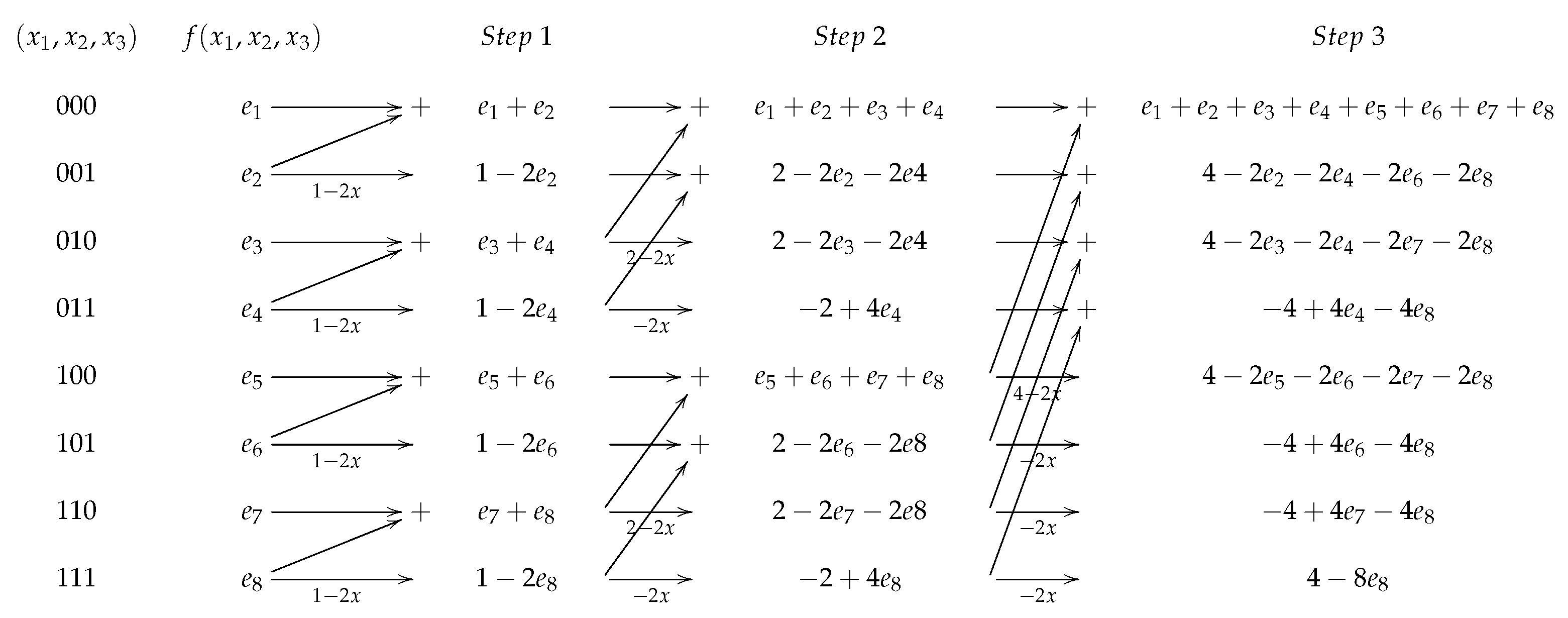
In Algorithm 4, we provide the pseudo code to compute the coefficients of the nonlinearity polynomial in $O\left(n{2}^n\right)$ integer operations. In Figure 1, Algorithm 4 is visualized for $n=3$.

Algorithm 4$\mathsf{NLP}$. Algorithm to calculate the nonlinearity polynomial ${\mathfrak{n}}_f$ in $O\left(n{2}^n\right)$ integer operations.

Input: The evaluation vector $\underline{f}$ of a B.f. $f(x_1,\dots ,x_n)$

Output: the vector $c=(c_1,\dots ,c_{2^{n+1}})$ of the coefficients of ${\mathfrak{n}}_f$

Calculation of the coefficients of the monomials not containing $a_0$

1: $(c_1,\dots ,c_{2^n})=\underline{f}$

2: for$i=0,\dots ,n-1$ do

3:  $b\leftarrow 0$

4:  repeat

5:    for $x=b,\dots ,b+2^i-1$ do

6:      $c_{x+1}\leftarrow c_{x+1}+c_{x+2^i+1}$

7:      if $x=b$ then

8:        $c_{x+2^i+1}\leftarrow 2^i-2c_{x+2^i+1}$

9:      else

10:        $c_{x+2^i+1}\leftarrow -2c_{x+2^i+1}$

11:      end if

12:    end for

13:    $b\leftarrow b+2^{i+1}$

14:  until $b=2^n$

15: end for

Calculation of the coefficients of the monomials containing $a_0$

16: $c_{1+2^n}\leftarrow 2^n-2c_1$

17: for$i=2,\dots ,2^n$ do

18:  $c_{i+2^n}\leftarrow -2c_i$

19: end for

20: return c

Theorem 5.

Algorithm 4 requires:

1.

$O\left(n{2}^n\right)$ integer sums and doublings, in particular about $n{2}^{n-1}$ integer sums and about $n{2}^{n-1}$ integer doublings.

2.

The storage of $O\left(2^n\right)$ integers of size less than or equal to $2^n$.

Proof. 

In the first part of Algorithm 4 (the computation of the coefficients of the monomials not containing $a_0$) the iteration on i is repeated n times. For each i, Step 9 and Step 11 or 13 are repeated $2^i\frac{2^n}{2^{i+1}}=2^{n/2}$ times (since b goes from 0 to $2^n$ by a step of $2^{i+1}$ and x performs $2^i$ steps). In Step 9 only one integer sum is performed, in Steps 11 we have one integer sum and one doubling, and in Step 13 only one doubling. Then the total amount of integer operation is $O\left(n{2}^n\right)$. Finally the computation of the coefficients of the monomials containing $a_0$ requires only $2^n$ integer doublings. To store all the monomials of the nonlinearity polynomial we have to store $2^{n+1}$ integers, although Corollary 1 shows that it is sufficient to store only the first half of them, i.e., $2^n$ integers. By Corollary 2, their size is less than or equal to $2^n$. □

5.2. Some Considerations on Algorithm 1

In Algorithm 1, almost all the computations are wasted evaluating all possible simple-t-monomials in $2^n$ variables, which are $\left(\genfrac{}{}{0pt}{}{2^n}{t}\right)$. This number grows enormously even for small values of n and t. We investigated experimentally how many of the $\left(\genfrac{}{}{0pt}{}{2^n}{t}\right)$ monomials are actually needed to compute the final Gröbner basis of $J_t^n$. Our experiment ran over all possible Boolean functions in 3 and 4 variables. The results are reported in

Table 3. Number of monomials needed to compute the Gröbner basis of the ideal $J_t^3$, using Algorithm 1: ${\mathsf{NL}}_{{\mathsf{GB}}_{\mathbb{F}}}$.

	${\mathit{J}}_1^3$				${\mathit{J}}_2^3$				${\mathit{J}}_3^3$
NL	#S	m	M	#C	#S	m	M	#C	#S	m	M	#C
0	4	4	4	8	0	0	0	0	0	0	0	0
1	4.5	4	5	4.4	8.5	7	10	28	0	0	0	0
2	4.4	4	5	4	9.7	8	11	24	9.3	8	11	56

,

Table 4. Number of monomials needed to compute the Gröbner basis of the ideal $J_t^4$, $t=1,2,3$, using Algorithm 1: ${\mathsf{NL}}_{{\mathsf{GB}}_{\mathbb{F}}}$.

	${\mathit{J}}_1^4$				${\mathit{J}}_2^4$				${\mathit{J}}_3^4$
NL	#S	m	M	#C	#S	m	M	#C	#S	m	M	#C
0	5	5	5	16	0	0	0	0	0	0	0	0
1	5.25	4	6	8	8.75	8	11	120	0	0	0	0
2	4.83	4	6	5.67	9.97	8	12	62.83	14.50	12	18	560
3	4.62	4	6	4.76	9.92	8	12	42.72	15.76	13	19	315.04
4	4.53	4	6	4.42	9.83	8	12	37.49	15.81	13	19	246.19
5	4.46	4	5	4.19	10.11	8	12	34.39	15.89	13	19	215.68
6	4.43	4	5	4.00	9.71	8	11	24.00	17.29	16	19	156.86

and

Table 5. Number of monomials needed to compute the Gröbner basis of the ideal $J_t^4$,$t=4,5,6,7$, using Algorithm 1: ${\mathsf{NL}}_{{\mathsf{GB}}_{\mathbb{F}}}$.

	${\mathit{J}}_4^4$				${\mathit{J}}_5^4$				${\mathit{J}}_6^4$				${\mathit{J}}_7^4$
NL	#S	m	M	#C	#S	m	M	#C	#S	m	M	#C	#S	m	M	#C
0	0	0	0	0	0	0	0	0	0	0	0	0	0	0	0	0
1	0	0	0	0	0	0	0	0	0	0	0	0	0	0	0	0
2	0	0	0	0	0	0	0	0	0	0	0	0	0	0	0	0
3	20.18	15	23	1820	0	0	0	0	0	0	0	0	0	0	0	0
4	21.44	16	24	1319.96	23.99	22	29	4368	0	0	0	0	0	0	0	0
5	21.54	19	24	1003.15	26.00	24	28	3851.24	23.50	22	25	8008	0	0	0	0
6	19.57	19	20	671.71	28	28	28	2603.79	28	28	28	7608.79	16	16	16	11441

. In this tables, for each $J_t^n$ there are four columns. Let $G_t^n$ be the Gröbner basis of $J_t^n$. Under the column labeled #C we report the average number of checked monomials in $2^n$ variables before obtaining $G_t^n$. Under the column labeled #S we report the average number of monomials which are actually sufficient to obtain $G_t^n$. Under the columns labeled “m” e “M” we report, respectively, the minimum and the maximum number of sufficient monomials to find $G_t^n$ running through all possible Boolean functions in n variables. For example, to compute the Gröbner basis of the ideal $J_2^3$ associated with a B.f. f whose nonlinearity is 2, we needed to check on average 24 monomials before finding the correct basis. Between the 24 monomials only $9.7$ (on average) were sufficient to obtain the same basis, where the number of sufficient monomials never exceeded the range 8–11.

5.3. Algorithms 1 and 2

Since it is not easy to estimate the complexity of a Gröbner basis computation theoretically, we give some experimental results, shown in

Table 6. Experimental comparisons of the coefficients of growth of the analyzed algorithms.

n	${log}_2\left[\frac{(\mathit{n}+1)2^{\mathit{n}+1}}{\mathit{n}{2}^{\mathit{n}}}\right]$	$\mathsf{FWT}$	${\mathsf{NL}}_{\mathsf{NLP}+\mathsf{FPE}}$ Algorithm 3	${\mathsf{NL}}_{{\mathsf{GB}}_{{\mathbb{F}}_{\mathsf{p}}}}$ Algorithm 2	${\mathsf{NL}}_{{\mathsf{GB}}_{\mathbb{Q}}}$ Algorithm 2	${\mathsf{NL}}_{{\mathsf{GB}}_{\mathbb{F}}}$ Algorithm 1
2–3	1.53	-	-	1.45	1.86	2.50
3–4	1.31	-	-	1.88	2.27	7.51
4–5	1.22	0.90	1.02	2.33	2.91	-
5–6	1.17	0.98	1.09	2.64	3.23	-
6–7	1.14	1.01	1.13	2.76	4.29	-
7–8	1.12	1.22	1.07	3.24	-	-
8–9	1.11	0.95	1.17	3.48	-	-
9–10	1.09	1.25	1.07	-	-	-
10–11	1.09	1.07	1.11	-	-	-

.

In this table we report the coefficients of growth of the analyzed algorithms (to compute the values in the columns $\mathsf{FWT}$ and ${\mathsf{NL}}_{\mathsf{NLP}+\mathsf{FPE}}$ we tested 15,000 random Boolean functions from $n=4$, since for $n=3$ there are only $2^{\left(2^3\right)}=256$ Boolean functions), comparing them with the value ${log}_2\left[\frac{(n+1)2^{n+1}}{n{2}^n}\right]$. For each algorithm we compute the average time $t_n$ to compute the nonlinearity of a B.f. with n variables and the average time $t_{n+1}$ to compute the nonlinearity of a B.f. with $n+1$ variables. Then we report in the table the value ${log}_2\left(\frac{t_{n+1}}{t_n}\right)$. When Gröbner bases are computed, then graded reverse lexicographical order is used, with Magma [39] implementation of the Faugère $F4$ algorithm [40]. Since the ideal $J_t^n\left(f\right)$ of Definition 9 is derived from the evaluation of $\left(\genfrac{}{}{0pt}{}{2^n}{t}\right)$ monomials (generating at most the same number of equations), then the complexity of Algorithm 1 is equivalent to the complexity of computing a Gröbner basis of at most $\left(\genfrac{}{}{0pt}{}{2^n}{t}\right)$ equations of degree d (where $1<d\le t$) in $n+1$ variables over the field $\mathbb{F}$. This method becomes almost impractical for $n=5$. We recall that $t\le 2^{n-1}-2^{\frac{n}{2}-1}$ (see Equation (2)).

The complexity of Algorithm 2 is equivalent to the complexity of computing a Gröbner basis of only $n+1$ field equations plus one single polynomial ${\mathfrak{n}}_f$ of degree at most $n+1$ in $n+1$ variables over the rational field, i.e., $\mathbb{K}=\mathbb{Q}$ (or over a prime field, i.e., $\mathbb{K}={\mathbb{F}}_p$) with coefficients of size less then or equal to $2^n$. As shown in Table 6, computing this Gröbner basis over a prime field ${\mathbb{F}}_p$ with $p\sim 2^n$ is much faster than computing the same base over $\mathbb{Q}$. It may be investigated if there exist better size for the prime p.

5.4. Algorithm 3

Theorem 6.

Algorithm 3 returns the nonlinearity of a B.f. f with n variables in $O\left(n{2}^n\right)$ integers operations (sums and doublings).

Proof. 

Algorithm 3 can be divided in three main steps:

• Calculation of the nonlinearity polynomial ${\mathfrak{n}}_f$. This step, as shown in Theorem 5, requires $O\left(n{2}^n\right)$ integer operations and $O\left(2^n\right)$ memory.
• Evaluation of the nonlinearity polynomial ${\mathfrak{n}}_f$. This step can be performed using fast Möbius transform in $O\left(n{2}^n\right)$ integer sums and $O\left(2^n\right)$ memory. We refer to this algorithm as the Fast Polynomial Evaluation ($\mathsf{FPE}$) algorithm.
• Computation of the minimum ${\mathfrak{n}}_f\left(a\right)$ with $a\in {\mathbb{Z}}^{n+1}$. This step requires no more than $O\left(2^n\right)$ checks.

The overall complexity is then $O\left(n{2}^n\right)$ integer operations and $O\left(2^n\right)$ memory. □

6. Conclusions

We presented three approaches to compute the nonlinearity of a Boolean function using multivariate polynomials. In particular we show that the problem of computing the distance of a generic B.f. f from the set of affine functions is equivalent to the problem of solving a multivariate polynomial system over the binary field. This system can be reformulated over the rationals by considering the associated pseudo Boolean function, and we can exhibit a multivariate polynomial whose evaluations solve the problem. Moreover, we evaluate our polynomial using fast Fourier techniques and solve the problem very efficiently. In particular, with our polynomial-based approach we compute the nonlinearity of any B.f. in $O\left(n{2}^n\right)$ operations, reaching the same asymptotic complexity of classical methods. The first of the presented methods returns the nonlinearity of f and a compact algebraic representation of all affine functions with distance t from f, opposed to traditional methods to compute the nonlinearity which only allow to deduce these affine functions from the Walsh table, not yielding a compact algebraic representation. Regarding the two other methods, they make use of a special polynomial, namely the nonlinearity polynomial, which is an interesting mathematical object per se. Studying his properties might open interesting research directions, and, possibly, finding a more efficient way of determining its minimum value, will determine a more efficient way of computing the nonlinearity.

References

- Shannon, C.E. Communication theory of secrecy systems. Bell Syst. Tech. J. 1949, 28, 656–715. [Google Scholar] [CrossRef]
- Rothaus, O.S. On “bent” functions. J. Comb. Theory Ser. A 1976, 20, 300–305. [Google Scholar] [CrossRef] [Green Version]
- Adams, C.M.; Tavares, S.E. The Use of Bent Sequences to Achieve Higher-Order Strict Avalanche Criterion in S-Box Design; Technical Report TR 90-013; Queen’s University: Kingston, ON, Canada, 1990. [Google Scholar]
- Maitra, S.; Sarkar, P. Maximum nonlinearity of symmetric Boolean functions on odd number of variables. IEEE Trans. Inf. Theory 2002, 48, 2626–2630. [Google Scholar] [CrossRef]
- Savickỳ, P. On the bent Boolean functions that are symmetric. Eur. J. Comb. 1994, 15, 407–410. [Google Scholar] [CrossRef] [Green Version]
- Cusick, T.W.; Stanica, P. Cryptographic Boolean Functions and Applications; Academic Press: Cambridge, MA, USA, 2017. [Google Scholar]
- Carlet, C. Boolean Functions for Cryptography and Coding Theory; Cambridge University Press: Cambridge, UK, 2021. [Google Scholar]
- Wu, C.-K.; Feng, D. Boolean Functions and Their Applications in Cryptography; Springer: Berlin/Heidelberg, Germany, 2016. [Google Scholar]
- Carlet, C.; Mesnager, S. Four decades of research on bent functions. Des. Codes Cryptogr. 2016, 78, 5–50. [Google Scholar] [CrossRef]
- Dillon, J.F. Elementary Hadamard Difference Sets. Ph.D. Thesis, University of Maryland, College Park, MD, USA, 1974. [Google Scholar]
- Tokareva, N. Bent Functions: Results and Applications to Cryptography; Academic Press: Cambridge, MA, USA; Elsevier: Amsterdam, The Netherlands, 2015. [Google Scholar]
- Carlet, C. Boolean functions for cryptography and error correcting codes, Boolean Models and Methods in Mathematics. Comput. Sci. Eng. 2010, 2, 257–397. [Google Scholar]
- Mesnager, S. Bent Functions; Springer: Berlin/Heidelberg, Germany, 2016. [Google Scholar]
- Çalık, Ç. Nonlinearity computation for sparse boolean functions. arXiv 2013, arXiv:1305.0860. [Google Scholar]
- Çalık, Ç. Computing Cryptographic Properties of Boolean Functions from the Algebraic Normal form Representation. Ph.D. Thesis, Middle East Technical University, Ankara, Turkey, 2013. [Google Scholar]
- Carlet, C. On the confusion and diffusion properties of Maiorana–McFarland’s and extended Maiorana–McFarland’s functions. J. Complex. 2004, 20, 182–204. [Google Scholar] [CrossRef] [Green Version]
- Dobbertin, H. Construction of bent functions and balanced Boolean functions with high nonlinearity. In International Workshop on Fast Software Encryption; Springer: Berlin/Heidelberg, Germany, 1994; pp. 61–74. [Google Scholar]
- Charpin, P. Normal boolean functions. J. Complex. 2004, 20, 245–265. [Google Scholar] [CrossRef] [Green Version]
- Carlet, C.; Méaux, P.; Rotella, Y. Boolean functions with restricted input and their robustness; application to the flip cipher. IACR Trans. Symmetric Cryptol. 2017, 2017, 192–227. [Google Scholar] [CrossRef]
- Carlet, C. Recursive lower bounds on the nonlinearity profile of boolean functions and their applications. IEEE Trans. Inf. Theory 2008, 54, 1262–1272. [Google Scholar] [CrossRef]
- Iwata, T.; Kurosawa, K. Probabilistic higher order differential attack and higher order bent functions. In International Conference on the Theory and Application of Cryptology and Information Security; Springer: Berlin/Heidelberg, Germany, 1999; pp. 62–74. [Google Scholar]
- Carlet, C. On the higher order nonlinearities of algebraic immune functions. In Annual International Cryptology Conference; Springer: Berlin/Heidelberg, Germany, 2006; pp. 584–601. [Google Scholar]
- Carlet, C.; Dalai, D.K.; Gupta, K.C.; Maitra, S. Algebraic immunity for cryptographically significant boolean functions: Analysis and construction. IEEE Trans. Inf. Theory 2006, 52, 3105–3121. [Google Scholar] [CrossRef]
- Yan, H.; Tang, D. Improving lower bounds on the second-order nonlinearity of three classes of boolean functions. Discret. Math. 2020, 343, 111698. [Google Scholar] [CrossRef]
- Mesnager, S.; Zhou, Z.; Ding, C. On the nonlinearity of boolean functions with restricted input. Cryptogr. Commun. 2019, 11, 63–76. [Google Scholar] [CrossRef]
- Semaev, I. New non-linearity parameters of boolean functions. arXiv 2019, arXiv:1906.00426. [Google Scholar]
- Guerrini, E.; Orsini, E.; Sala, M. Computing the distance distribution of systematic nonlinear codes. J. Algebra Its Appl. 2010, 9, 241–256. [Google Scholar] [CrossRef] [Green Version]
- Bellini, E.; Sala, M. A deterministic algorithm for the distance and weight distribution of binary nonlinear codes. Int. J. Inf. Coding Theory 2018, 5, 18–35. [Google Scholar]
- Sala, M.; Simonetti, I. An algebraic description of Boolean Functions. International Workshop on Coding and Cryptography (WCC) 2007, Versailles, France, 2007. Available online: https://citeseerx.ist.psu.edu/viewdoc/download?doi=10.1.1.74.3211&rep=rep1&type=pdf (accessed on 2 November 2021).
- Bellini, E.; Mora, T.; Sala, M. Algorithmic Approach Using Polynomial Systems for the Nonlinearity of Boolean Functions, Computation Presentation. In Proceedings of the The thirteen conference on Effective Methods in Algebraic Geometry, Trento, Italy, 15–19 June 2015. [Google Scholar]
- Bellini, E. Yet Another Algorithm to Compute the Nonlinearity of a Boolean Function. In Proceedings of the Yet Another Conference on Cryptography, Porquerolles, France, 9–13 June 2014; Available online: http://veron.univ-tln.fr/YACC14/Bellini.pdf (accessed on 2 November 2021).
- MacWilliams, F.J.; Sloane, N.J.A. The Theory of Error-Correcting Codes; North-Holland Publishing Co. Amsterdam, North-Holland Mathematical Library: Amsterdam, North-Holland, 1977; Volume 16. [Google Scholar]
- Carlet, C.; Guillot, P. A new representation of Boolean functions. In Applied Algebra, Algebraic Algorithms and Error-Correcting Codes; Springer: Berlin/Heidelberg, Germany, 1999; pp. 94–103. [Google Scholar]
- Carlet, C.; Guillot, P. Bent, resilient functions and the Numerical Normal Form. DIMACS Ser. Discret. Math. Theor. Comput. Sci. 2001, 56, 87–96. [Google Scholar]
- Carlet, C. On the coset weight divisibility and nonlinearity of resilient and correlation-immune functions. In Sequences and Their Applications; Springer: Berlin/Heidelberg, Germany, 2002; pp. 131–144. [Google Scholar]
- Simonetti, I. On the non-linearity of Boolean functions. In Gröbner Bases, Coding, and Cryptography; RISC Book Series; Sala, M., Mora, T., Perret, L., Sakata, S., Traverso, C., Eds.; Springer: Heidelberg, Germany, 2009; pp. 409–413. [Google Scholar]
- Guerrini, E. On Distance and Optimality in Non-Linear Codes. Master’s Thesis, Department of Mathematics, University of Pisa, Pisa, Italy, 2005. [Google Scholar]
- Seidenberg, A. Constructions in algebra. Trans. Amer. Math. Soc. 1974, 197, 273–313. [Google Scholar] [CrossRef]
- MAGMA: Computational Algebra System for Algebra, Number Theory and Geometry, The University of Sydney Computational Algebra Group. 2020. Available online: http://magma.maths.usyd.edu.au/magma (accessed on 16 December 2021).
- Faugere, J.-C. A new efficient algorithm for computing gröbner bases (f4). J. Pure Appl. Algebra 1999, 139, 61–88. [Google Scholar] [CrossRef]
- Simonetti, I. On Some Applications of Commutative Algebra to Boolean Functions and Their Non-Linearity. Ph.D. Thesis, Department of Mathematics, University of Trento, Trento, Italy, 2007. [Google Scholar]
- Bellini, E. Computational Techniques for Nonlinear Codes and Boolean Functions. Ph.D. Thesis, Department of Mathematics, University of Trento, Trento, Italy, 2014. [Google Scholar]
Figure 1.
Butterfly scheme to efficiently compute the coefficients of the nonlinearity polynomial, where (see Algorithm 4: ).