
Rotational Cryptanalysis on ChaCha Stream Cipher


1
Department of Mathematical Sciences “Giuseppe Luigi Lagrange”, Politecnico di Torino, 10129 Torino, Italy
2
Cryptography Research Centre, Technology Innovation Institute, Abu Dhabi P.O. Box 9639, United Arab Emirates
*
Author to whom correspondence should be addressed.
Symmetry 2022, 14(6), 1087; https://0-doi-org.brum.beds.ac.uk/10.3390/sym14061087
Submission received: 17 March 2022
/
Revised: 13 May 2022
/
Accepted: 20 May 2022
/
Published: 25 May 2022
(This article belongs to the Special Issue The Advances in Algebraic Coding Theory)
Abstract
:In this paper we consider the ChaCha20 stream cipher in the related-key scenario and we study how to obtain rotational-XOR pairs with nonzero probability after the application of the first quarter round. The ChaCha20 input can be viewed as a matrix of 32-bit words, where the first row of the matrix is fixed to a constant value, the second two rows represent the key, and the fourth some initialization values. Under some reasonable independence assumptions and a suitable selection of the input, we show that the aforementioned probability is about , a value greater than , which is the one expected from a random permutation. We also investigate the existence of constants, different from the ones used in the first row of the ChaCha20 input, for which the rotational-XOR probability increases, representing a potential weakness in variants of the ChaCha20 stream cipher. So far, to our knowledge, this is the first analysis of the ChaCha20 stream cipher from a rotational-XOR perspective.
MSC:
Primary: 94A60; 11T71; Secondary: 11T06; 94D101. Introduction
The ChaCha20 stream cypher, published in 2008 [1], was developed by Daniel J. Bernstein as a modification of Salsa20 [2], another stream cypher designed in 2005 by the same author and then later submitted to the eSTREAM project. The aim of ChaCha20 is to increase diffusion and performance on some architectures with respect to Salsa20. Google has selected ChaCha20 along with Bernstein’s Poly1305 message authentication code as a replacement for RC4 in TLS, and its specifications can be found in [3]. Both ciphers are ARX (Add-Rotate-XOR) ciphers, i.e., built on a pseudorandom function based only on the following three 32-bit word operations: modular addition, circular rotation, and bitwise exclusive or (XOR). This pseudorandom function is itself built upon a 512 bit permutation. According to [4], both permutations are not designed to simulate ideal permutations: they are designed to simulate ideal permutations with certain symmetries, i.e., ideal permutations of the orbits of the state space under these symmetries. The input of the ChaCha20 function is partially fixed to specific asymmetric constants, ensuring that different inputs lie in different orbits. As a consequence of the ChaCha20 design, some cryptanalytic techniques, such as rotational cryptanalysis, seem hard to apply.
Related works. Rotational cryptanalysis studies the propagation of rotational pairs throughout the encryption steps of an ARX scheme. It is a probabilistic chosen-plaintext attack that turns to be an effective cryptanalytical tool against ciphers and hash functions that are based on the three ARX operations.
A rotational pair of keys was considered for the first time in the pioneering work on related keys by Biham [5]. This approach was extended by Kelsey et al. in several related-key attacks on block ciphers [6]. A rotational pair of inputs was later adopted in the cryptanalysis of the compression function of Shabal [7] (the term “rotational input” was not used yet), but it was traced only through bitwise operations and not through additions. Bernstein [8] explicitly prevented using rotational pairs in Salsa20 (and ChaCha20) by fixing non-symmetric constants in the input of the permutation. However, he did not provide any complexity or probability estimates for this kind of attack. The designers of the block cipher SEA [9] described the technique of rotational cryptanalysis in 2006 and defended against it with non-linear key-schedule and pseudorandom constants. In his Ph.D. thesis, Daum [10] described the links between modular addition and bit rotations. In 2010, the term “rotational cryptanalysis” appeared for the first time in the papers of Khovratovich and Nikolić [11,12], were they cryptanalyzed the reduced-round Threefish cipher, which is part of the Skein hash function, a SHA-3 competition candidate [13]. Their attack covered 53 rounds of Skein-256 and 57 rounds of Skein-512. In the aforementioned paper [11], the authors proved that for ARX primitives, under the assumption that the cipher can be modeled as a Markov chain, the probability to have a rotational pair of inputs which will produce a rotational pair at the output depends on the number of additions only. This claim was corrected in [14], where the authors showed that chained modular additions used in ARX ciphers do not always form a Markov chain with regards to rotational analysis. They provided a precise value of the probability of such chains and they gave a new algorithm for computing the rotational probability of ARX ciphers. Then, they used the algorithm to correct (from 12 to 7 rounds) the rotational attacks on BLAKE2 [15] and to provide valid rotational attacks against the simplified version of Skein. In 2013, rotational cryptanalysis was also applied to distinguish four rounds of KECCAK permutation [16] in time . A crucial requirement for rotational cryptanalysis to work effectively is that all constants used in the ARX primitive must preserve their values when rotated. This requirement can be relaxed to some extent and instead of assuming completely rotational constants, one can work with constants that are almost rotational, i.e., the XOR difference between the initial constants and the rotated ones gives words of small Hamming weight. A different approach was taken by Ashur and Liu in 2016 [17]. They presented a way to compute the rotational probability when constants are injected into the state and applied their approach to Speck. In particular, they exposed, in the related-key scenario, a trail suggesting that a weak key class of size exists, leading to a 7-round distinguisher for Speck64/32. The technique was later automated in [18], through the use of SAT solvers. In [19], a rotational cryptanalysis of the Salsa core function was presented, also finding rotational distinguishers for the Salsa and Chacha permutations: the rotational distinguisher for the ChaCha permutation performs properly only up to 8 rounds with a probability of approximately , while the rotational distinguisher for the Salsa permutation performs properly up to 32 rounds with a probability of approximately , clarifying the weakness of the Salsa core function with respect to rotational cryptanalysis. Finally, in [20] the authors applied rotational cryptanalysis to Chacha20 permutation without considering the injected constants in the state of the permutation, showing that it does not behave as a random permutation for up to 17 rounds, since the related probability is less than for 17 rounds of ChaCha permutation, while, for a random permutation of the same input size, this probability is .
Our contribution. In this paper we study the applicability to the ChaCha20 stream cipher quarter round function of the techniques due to Ashur and Liu [17], used for the rotational cryptanalysis of Speck in the presence of constants. In order to do this, we first consider the quarter round function of Chacha20, described in Section 2, determining the conditions which guarantee that, starting from randomly and independently chosen -bit words, inputs and a -bit constant giving the –bit words as output, i.e.,
we can find a characteristics of the type
for some input relations , , where is an integer less than the word size and are -bit strings. Then, we search for a suitable selection of and key/nonce/counter relations, the above mentioned input relations , , such that, fixing the rotational amount , we can precisely determine which input constants yield rotational-XOR pairs with high or low probability, in a related-key scenario. We determine a formula to compute this probability as a function of and we show that in the case of the constants commonly used in ChaCha20 it is greater than , revealing the non-randomness of the quarter round permutation. Moreover we investigate the value of this probability for different constants than the ones injected in the ChaCha20 initial state, determining for which of them it increases. While in [19,20] it was only considered the core of ChaCha/Salsa, not the full stream cipher construction, to our knowledge, this is the first attempt to apply rotational analysis to the Chacha20 stream cipher in order to distinguish the behavior of the Chacha20 quarter round from a random permutation and to relate this behaviour to the values of the constants used in Chacha20.
Outline of the paper. In Section 2, we introduce the notation and the essential preliminaries, describing the ChaCha20 stream cipher and the fundamentals of rotational and rotational-XOR cryptanalysis.
In Section 3 we present our analysis. In particular, in Section 3.1, we derive a set of necessary and sufficient conditions which need to be satisfied for a rotational-XOR pair to appear in the output of ChaCha20 quarter round, given that the first word of the input is fixed to a constant value. In Section 3.2, we discuss a suitable choice of the input relations , and of the parameters allowing them to meet the above conditions.In Section 3.3, under the previous choice we compute the probability that these conditions are satisfied by a randomly and independently chosen set of inputs , , as a function of the constant , i.e., the probability that rotational-XOR pairs (with rotational amount ) appear as outputs of the quarter round. In Section 4 we discuss and resume our results. In particular, in Section 4.1 we evaluate this probability for the special constants commonly used in the ChaCha20 stream cipher. We show that, in our scenario, rotational-XOR pairs can appear in ChaCha20 after one round with probability around against the value of for a random permutation. In Section 4.2 we describe the form of some initial constants for which these pairs are very likely. Finally, in Section 5 we give our conclusions.
2. Notation and ChaCha20 Stream Cipher Description
In this section, we first define our notation, then we describe the specifications of the ChaCha20 stream cipher and we provide the basics of rotational and rotational-XOR cryptanalysis.
2.1. Notation
Let be the binary field with two elements, and be the set of all matrices with elements in . Depending on the context, lowercase letters stand for -bit words or for the corresponding non-negative integers they represent, i.e.,
where for all . In the case of ChaCha20, we have and . With uppercase letters we indicate a matrix of words, i.e., .
We also use the following notation:
- ⊕ for the bitwise exclusive or (XOR), i.e., the addition in ;
- ⊞ for the -bit addition ;
- ⊟ for the -bit subtraction , i.e., the sum with the opposite of an element in ;
- for the -bit addition of k words ;
- for the vector bitwise OR operation between x and y;
- for the concatenation of x and y;
- for a non–cyclic left shift by one bit of x;
- ;
- and respectively for constant-distance left and right circular rotation of bits of a -bit word with ;
- for the Hamming weight of x;
- for the cardinality of a set I;
- for the characteristic function of a condition Z, which is equal to 1 when Z is satisfied and equal to 0 otherwise;
- ;
- if and only if we have for all ;
- , where, for ,and, considering ,with and ;
- for the operator which gives for any the integer satisfying
2.2. ChaCha20 Specification
The ChaCha20 permutation has a state of 512 bits, which can be seen as a matrix whose elements are binary vectors of bits, i.e.,
The initial state of ChaCha20 is initialized by setting the first row to a 128-bit constant value, the second and third row are used to store a 256-bit key, and the fourth row contains a 64-bit nonce and a 64-bit counter.
Definition 1
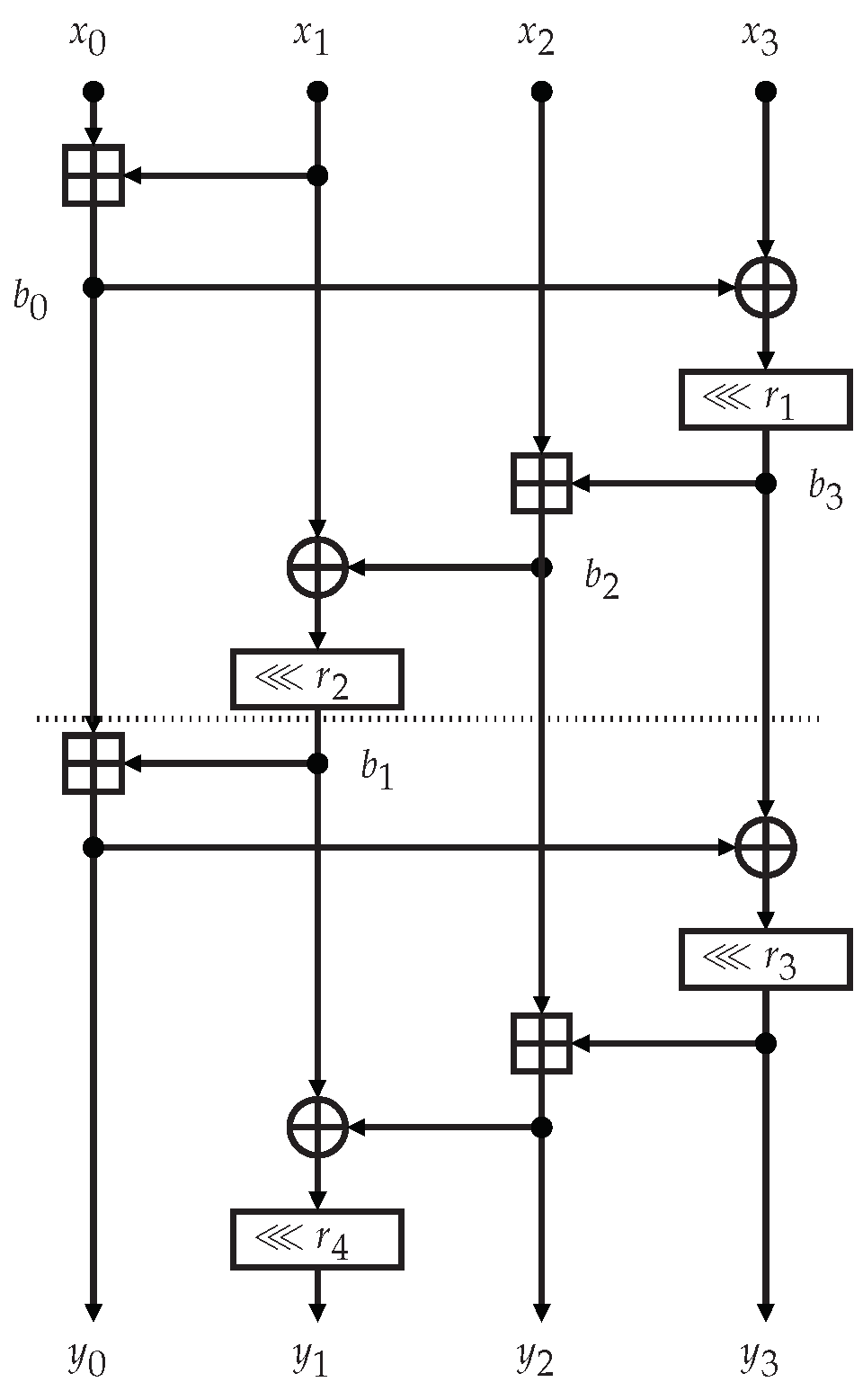
(ChaCha20 quarter round). Let be -bit words, and let , where is the ChaCha20 quarter round, defined as follows:
We show in Figure 1 a schematic drawing of the ChaCha20 quarter round. The permutation used in the ChaCha20 stream cipher performs 20 rounds or, equivalently, 10 double rounds. Two consecutive rounds (or a double round) of the ChaCha20 permutation consist in applying the quarter round four times in parallel to the columns of the state (first round), and then four times in parallel to the diagonals of the state (second round). More formally:
Definition 2
(ChaCha20 column/diagonal round). Let , be two matrices in .
A column round is defined as follows, with :
A diagonal round is defined as follows, for and where each subscript is computed modulo :
2.3. Rotational and Rotational-XOR (RX) Cryptanalysis
Rotational cryptanalysis is essentially a distinguishing attack that exploits rotational offsets with probability higher than the one for a random permutation. If we consider a –bit word x and a rotational offset , we call a rotational pair and we define the rotational property as the property that an operation with the input of a rotational pair gives, as output, another rotational pair. Let us denote with an ARX scheme with q modular additions. Rotational cryptanalysis is based on the following facts:
- The rotational property is preserved through the XOR of rotational pairs and after a rotation by a constant value :
- The rotational property is preserved through a modular addition of two –bit words with a probability given byand computed in Corollary 4.12 of [10], this probability is a decreasing function of , thus it is maximized when ;
- In the case of chained modular additions of more than two –bit strings, must be evaluated using Lemma 2 in [14];
- with probability
- Given a random function , with probability
Thus, we can detect non-randomness in the ARX scheme if . For example, when , an ARX scheme implemented with q not chained additions is vulnerable to rotational cryptanalysis if .
Rotational-XOR cryptanalysis is also a distinguishing attack, firstly introduced in [17] where it was applied to SPECK. This attack studies the propagation of a rotational-XOR pair (RX–pair), i.e., a couple having RX–difference . Clearly RX cryptanalysis is a generalization of rotational cryptanalysis, since they coincide when . Moreover for RX–pairs and we have
- ;
- for a fixed rotational amount .
The propagation of RX–differences through modular addition when can be computed using the following theorem proved in [17], whose statement has been adapted to our notation
Theorem 1
(Ashur-Liu [17]). Let be independent random variables. Let the following be constants in . Then the probability
when and is sufficiently large is equal to
where
and , .
3. Searching for Rotational/RX Pairs in ChaCha20
The aim of this section is to consider the ChaCha20 stream cipher, in which the first row in its initial state has constant entries, giving general conditions on the propagation of rotational/RX–pairs that we simply call rotational propagation. Moreover, by a suitable choice of inputs and parameters, we find a special case in which the rotational propagation can have a non-negligible probability depending on a certain family of these constants.
3.1. Conditions for the Rotational Propagation
Recalling that the first row of the ChaCha20 matrix has constant entries, the following proposition holds
Proposition 1.
Let us consider the ChaCha20 quarter round , a constant –bit string and the rotational amount with . If we have
and we consider the –bit strings and the entries , then
We call input relations the functions , .
Proof.
If we use the input instead of the input , we find
We have to satisfy the following conditions
where (11) and (13) easily give
from conditions and
since we have the condition . Now from (14) and (7) we find
and from (15) and (9) we have
Thus, the four conditions we need to satisfy are (16), (17), (10) and (12). If in (16) we substitute (6) and we take in account (1) in Definition 1, we find the first condition of our thesis
Finally if we substitute (11), (8), (14) and (2) in (12) we have the last condition of our thesis
□
3.2. On the Choices of the Input Relations and of a, b, c, d
One can consider many different choices for the values of and in order to satisfy the conditions of Proposition 1. Our intention is to set these values in order to obtain simplified conditions which can be satisfied with a non-negligible probability depending on the values given to . Considering Equations (14) and (15), a first simplification we apply is to choose a, b, c and d such that
With this setting the conditions of Proposition 1 become
and we have (21) and (22) satisfied when
Regarding the input relations, we consider expressions of the kind , which seem reasonable choices once we look to the remaining conditions (19) and (20). Indeed we may select and as
in order to simplify (19) and to give an expression for (20) very similar to the condition of rotational propagation through modular addition, obtaining
Now we have to think about and, consequently, about how to manage conditions (25) and (26). Clearly a possibility is to choose in order to reduce (26) exactly to the condition for the rotational propagation through modular addition
In this case (25) becomes
which holds for some only under particular conditions on . These conditions turn out to be too restrictive for our purposes. At the end of this subsection, we will prove them in Proposition 2, explaining why they give rise to a small number of possible choices for in order to obtain nonzero probability for (25). This part can be skipped over by the reader without problems. Therefore we may choose as something different from and consequently we may consider (26) as a condition of the form
where in general is not a constant, since it depends on . But we may combine the law of total probability with the Ashur-Liu Theorem 1 in [17] in order to find a probability estimate for (29) in the case . So a good choice is to consider the case and use (25) in order to define as we will do in the next subsection.
Proposition 2.
If we consider
and
then condition (28) holds if and only if we have
or, in other words, if and only if
Proof.
Following this choice, with arguments similar to the ones used by Daum in [10], we may evaluate some probability different from zero for condition (28) only when one of the following conditions is satisfied
- , i.e., which is equivalent to the equationand it gives possible values for ;
- , i.e., , , which is equivalent to the equationand it gives one value for only when and otherwise it is impossible;
- , i.e., , which is equivalent to the equationand it gives possible values for ;
- , i.e., , , which is equivalent to the equationand it gives one value for only when and otherwise it is impossible.
The strong dependence from of the possible values of for which (25) holds for some seems too limiting for our purposes. For example, when we have only two suitable values for from the third case and only a single value from the remaining ones.
3.3. Probability of Rotational Propagation for 1 Bit Rotations
From what we have previously pointed out, we will consider from now on with the choices (24), (35) and (29), where
and we use condition (25) in order to define
This definition of seems reasonable since we can simultaneously have (25) automatically satisfied and a better range of possible values for that may give a non-negligible probability for condition (26).
We will follow this path: first we will prove the following Corollary 1 of Theorem 1, then we will use it together with the law of total probability in order to find a formula for the probability of (29) depending on and in particular on the cardinalities of some sets related to . Finally, we will evaluate these cardinalities in Lemma 1 and we will give in Theorem 2 the value of this probability making explicit its dependence on .
Corollary 1.
Let be independent random variables, and
a constant word in . If j, , is the index of the first bit equal to 0 in starting from the right to the left, with the convention that only when has all the entries equal to 1, then
where
Proof.
We obtain if and only if we have
and, for all ,
Clearly, condition (41) holds when all the bits are equal to 1 for any , while, if , , is the first bit equal to 0 in starting from the right to the left, condition (41) holds for if and only if . Thus in order to have , we need such that , where all the first j bits from to are equal to 1 and the remaining ones from to are equal to 0, or , i.e., all the bits of are equal to 1. In these cases we find from Theorem 1 that On the other hand is equal to 1 if and only if we have
and for all condition (41) holds. Since in (41) implies and we have , an easy inductive argument shows that all the bits of must be equal to 0 in order to have . Thus and we find from Theorem 1 We finally observe that the two characteristic functions and can not be contemporarily equal to 1, and they are contemporarily equal to 0, with , for any other value of different from the ones we have pointed out. □
Thanks to the law of total probability, since for a fixed v we may assume as a constant while and are independent variables, we find
where we used the fact that is uniformly distributed, so . In order to explicitly evaluate applying the results of Corollary 1, we now define sets of –bit words having a special form and, in the next Lemma 1, we will find their cardinalities, depending on .
Definition 3.
Let us consider the vectors such that
We define the sets as
Therefore, from Corollary 1 we have the following explicit expression for
where, for , we evaluate the cardinalities in the following lemma.
Proof.
First of all, we recall that if and only if
or, equivalently, if and only if
and if we use (35) we finally have the condition
If we consider
we find
where . On the other hand, we have
and, since
where , and by Definition 3
we obtain
where .
Therefore, comparing (48) and (50), we find that condition (46) is equivalent to the system of congruences
where, using (47) and (49), and observing that
we can rewrite the first congruence of (51) as
Now, in solving (52) we have to consider the following cases.
- : in this case when congruence (52) becomesComparing the two members it clearly holds if and only ifand, by definition of , the second congruence in (51) holds ifwhere is fixed by (53) and by the free choice of . Therefore we always have only 2 solutions when . When congruence (52) becomesgiving and conditions similar to (53)and the same conditions (54) for congruence (51). Thus also when we find that we do not have conditions on and we always have only 2 solutions. Finally if both members of the congruence (52) are less than and they have the same parity if and only if . Moreover, we havewhere the equality holds if and only if for all , andwhere the equalities hold if for all . Thus we findwhich gives for all and, if , we need for all and . Therefore we have solutions only when the constant is such that for all and, since also in these cases the same conditions (54) for congruence (51) hold, we have free for all and possible solutions.
- : in this case we necessarily have and since only when , thus (52) becomesand we have solutions only when , in order to preserve the same parity for both members. Under this supplementary condition, congruence (55) is equivalent tomoreover in this case the second congruence in (51) givesori.e., for every solution of (56) we have also two possibilities for . Thus, since (56) can be solved as in the previous case distinguishing between , , and , the number of solutions is doubled. So, if and , we find 4 solutions, while, if and for all , we have solutions.
- : in this last case we have in the first congruence in (51) so this congruence becomes the equalitySinceif we have solutions only when for all and , with the two possibilities for given byorso all are solutions. On the other hand, if and , from (57) we also need for all and , therefore and . Thus only is fixed and we have solutions. Finally, when and we also need for all and . Therefore and , thus also in this case we have only fixed and, consequently, there are solutions.
□
Thanks to Lemma 1 and to (44), we have nonzero probabilities only if satisfies one of the following conditions
- ,
- and ,
- , , i.e., is the zero vector in ,
or, in other words, there are possible choices of which are about of all the possible constants.
In the following theorem we give the exact values of excluding the only three trivial values of for which .
Theorem 2.
Let us consider such that for all with and different from , , . Then we have
where
Proof.
With our choices of and from the results of Lemma 1, we have for , for if , and if . Thus, from (44) we obtain
If from the results of Lemma 1 we find
and, since
an easy calculation gives
The case and is straightforward, since all the non-zero cardinalities of the sets are doubled. □
4. Discussion
- conditions (21) and (22) hold automatically from (23);
Therefore when and is sufficiently large, if satisfies the hypotheses of Theorem 2 and following our choices for , , , a, b, c and d, with the aforementioned assumptions of independence and uniform distribution for , and , the equality
holds with probability given by (58).
4.1. Propagation Probability of Rotational-XOR Pairs through ChaCha20 Quarter Round
If we consider the four constants used in the ChaCha20 definition, they all satisfy , thus we have
- and , so , which gives when ;
- and with as before;
- and , , so , which gives when ;
- and with as for the first two constants.
A simple calculation shows that the probability of rotational propagation related to the 4 columns of the initial state of ChaCha20 is which is greater than .
4.2. ChaCha20 Alternative Constants Giving Non-Negligible Probability
In our scenario, this probability increases for some selections of alternative constants and may represent a weakness for variants of ChaCha20 against rotational attacks. From Theorem 2 we observe that has always a higher value when . In this case we find
both of them are greater than for all the possible values of and increase their value when t decreases. Thus, constants satisfying the hypotheses of Theorem 2 and giving a rotational propagation probability for the quarter round greater than when have one of the two following forms
Finally, we consider the following special values of :
5. Conclusions
We considered the ChaCha20 stream cipher and we studied the propagation of rotational-XOR pairs in the quarter round function. Under suitable choices of the inputs and assumptions of independence and uniform distribution, setting the rotational amount to 1, we established a formula for the probability of the propagation of rotational-XOR pairs depending on the selected constants. For the standard constants in ChaCha20 we find a probability around against the probability of of a random permutation. Moreover, we were able to find a family of constants which in our scenario potentially facilitate rotational propagation with non-negligible probability.
Author Contributions
Conceptualization, S.B., D.B. and E.B.; methodology, S.B. and E.B.; validation, S.B. and E.B.; formal analysis, S.B. and E.B.; investigation, S.B., D.B. and E.B.; resources, D.B. and E.B.; data curation, S.B. and E.B.; writing—original draft preparation, S.B.; writing—review and editing, S.B. and E.B.; visualization, S.B. and E.B.; supervision D.B. and E.B.; project administration, D.B. and E.B.; funding acquisition, D.B. All authors have read and agreed to the published version of the manuscript.
Funding
This research was funded by Politecnico di Torino (Funding for basic research).
Institutional Review Board Statement
Not applicable.
Informed Consent Statement
Not applicable.
Data Availability Statement
Not applicable.
Acknowledgments
The authors would like to thank the anonymous referees for their valuable suggestions and corrections which surely improved the paper.
Conflicts of Interest
The authors declare no conflict of interest.
References
- Bernstein, D.J. ChaCha, a Variant of Salsa20. In Workshop Record of SASC; 2008; Volume 8, pp. 3–5. Available online: https://cr.yp.to/chacha/chacha-20080120.pdf (accessed on 23 May 2022).
- Bernstein, D.J. Salsa20 Specification. In Technical Report, eSTREAM Project; 2005; Available online: http://www.ecrypt.eu.org/stream/salsa20pf.html (accessed on 23 May 2022).
- Nir, Y.; Langley, A. Chacha20 and poly1305 for IETF protocols. RFC 2018, 8439, 1–46. [Google Scholar] [CrossRef]
- Bernstein, D.J.; Hopwood, D.; Hülsing, A.; Lange, T.; Niederhagen, R.; Papachristodoulou, L.; Schneider, M.; Schwabe, P.; Wilcox-O’Hearn, Z. SPHINCS: Practical Stateless Hash–Based Signatures. In Advances in Cryptology—EUROCRYPT 2015; LNCS; Springer: Berlin/Heidelberg, Germany, 2015; Volume 9056, pp. 368–397. [Google Scholar] [CrossRef] [Green Version]
- Biham, E. New Types of Cryptanalytic Attacks Using Related Keys. J. Cryptol. 1994, 7, 229–246. [Google Scholar] [CrossRef]
- Kelsey, J.; Schneier, B.; Wagner, D. Related-key cryptanalysis of 3-way, biham-DES, CAST, DES-X, newDES, RC2, and TEA. In Information and Communications Security. ICICS 1997; LNCS; Springer: Berlin/Heidelberg, Germany, 1997; Volume 1334, pp. 233–246. [Google Scholar] [CrossRef]
- Knudsen, L.R.; Matusiewicz, K.; Thomsen, S.S. Observations on the Shabal Keyed Permutation. In Official Comment. 2009. Available online: http://www2.mat.dtu.dk/people/oldusers/S.Thomsen/shabal/shabal.pdf (accessed on 23 May 2022).
- Bernstein, D.J. Salsa20 Security. In Technical Report, eSTREAM Project; 2005; Available online: http://cr.yp.to/snuffle/security.pdf (accessed on 23 May 2022).
- Standaert, F.-X.; Piret, G.; Gershenfeld, N.; Quisquater, J.-J. Sea: A Scalable Encryption Algorithm for Small Embedded Applications. In Smart Card Research and Advanced Applications. CARDIS 2006; LNCS; Springer: Berlin/Heidelberg, Germany, 2006; Volume 3928, pp. 222–236. [Google Scholar] [CrossRef] [Green Version]
- Daum, M. Cryptanalysis of Hash Functions of the MD4-Family. Ph.D. Thesis, Ruhr University Bochum, Bochum, Germany, 2005. Available online: http://citeseerx.ist.psu.edu/viewdoc/download?doi=10.1.1.88.7847&rep=rep1&type=pdf (accessed on 23 May 2022).
- Khovratovich, D.; Nikolić, I. Rotational cryptanalysis of ARX. In Fast Software Encryption. FSE 2010; LNCS; Springer: Berlin/Heidelberg, Germany, 2010; Volume 6147, pp. 333–346. [Google Scholar] [CrossRef] [Green Version]
- Khovratovich, D.; Nikolić, I.; Rechberger, C. Rotational Rebound Attacks on Reduced Skein. In Advances in Cryptology—ASIACRYPT 2010; LNCS; Springer: Berlin/Heidelberg, Germany, 2010; Volume 6477, pp. 1–19. [Google Scholar] [CrossRef] [Green Version]
- Ferguson, N.; Lucks, S.; Schneier, B.; Whiting, D.; Bellare, M.; Kohno, T.; Callas, J.; Walker, J. The Skein Hash Function Family. Submiss. NIST (Round 3) 2010, 7, 3. [Google Scholar]
- Khovratovich, D.; Nikolić, I.; Pieprzyk, J.; Sokolowski, P.; Steinfeld, R. Rotational Cryptanalysis of ARX Revisited. In Fast Software Encryption. FSE 2015; LNCS; Springer: Berlin/Heidelberg, Germany, 2015; Volume 9054, pp. 519–536. [Google Scholar] [CrossRef] [Green Version]
- Guo, J.; Karpman, P.; Nikolić, I.; Wang, L.; Wu, S. Analysis of BLAKE2. In Topics in Cryptology—CT-RSA 2014; LNCS; Springer: Cham, Switzerland, 2014; Volume 8366, pp. 402–423. [Google Scholar] [CrossRef]
- Morawiecki, P.; Pieprzyk, J.; Srebrny, M. Rotational Cryptanalysis of Round-reduced Keccak. In Fast Software Encryption: 20th International Workshop; LNCS; Springer: Berlin/Heidelberg, Germany, 2013; Volume 8424, pp. 241–262. [Google Scholar] [CrossRef] [Green Version]
- Ashur, T.; Liu, Y. Rotational Cryptanalysis in the Presence of Constants. IACR Trans. Symmetric Cryptol. 2016, 2016, 57–70. [Google Scholar] [CrossRef]
- Ashur, T.; De Witte, G.; Liu, Y. An Automated Tool for Rotational-XOR Cryptanalysis of ARX-based Primitives. In Proceedings of the 2017 Symposium on Information Theory and Signal Processing in the Benelux (SITB 2017), Delft, The Netherlands, 11–12 May 2017. [Google Scholar]
- Ito, R. Rotational Cryptanalysis of Salsa Core Function. In Information Security. ISC 2020; LNCS; Springer: Cham, Switzerland, 2020; Volume 12472, pp. 129–145. [Google Scholar] [CrossRef]
- Barbero, S.; Bellini, E.; Makarim, R. Rotational Analysis of ChaCha Permutation. Adv. Math. Commun. 2021. [Google Scholar] [CrossRef]
Figure 1.
The ChaCha20 quarter round scheme.

Publisher’s Note: MDPI stays neutral with regard to jurisdictional claims in published maps and institutional affiliations. |
© 2022 by the authors. Licensee MDPI, Basel, Switzerland. This article is an open access article distributed under the terms and conditions of the Creative Commons Attribution (CC BY) license (https://creativecommons.org/licenses/by/4.0/).
Share and Cite
MDPI and ACS Style
Barbero, S.; Bazzanella, D.; Bellini, E. Rotational Cryptanalysis on ChaCha Stream Cipher. Symmetry 2022, 14, 1087. https://0-doi-org.brum.beds.ac.uk/10.3390/sym14061087
AMA Style
Barbero S, Bazzanella D, Bellini E. Rotational Cryptanalysis on ChaCha Stream Cipher. Symmetry. 2022; 14(6):1087. https://0-doi-org.brum.beds.ac.uk/10.3390/sym14061087
Chicago/Turabian StyleBarbero, Stefano, Danilo Bazzanella, and Emanuele Bellini. 2022. "Rotational Cryptanalysis on ChaCha Stream Cipher" Symmetry 14, no. 6: 1087. https://0-doi-org.brum.beds.ac.uk/10.3390/sym14061087
Note that from the first issue of 2016, this journal uses article numbers instead of page numbers. See further details here.