
Moving Forward by Shaking Sideways


Department of Mathematics, University of Wisconsin–Madison, 480 Lincoln Dr., Madison, WI 53706, USA
Symmetry 2022, 14(3), 620; https://0-doi-org.brum.beds.ac.uk/10.3390/sym14030620
Submission received: 24 February 2022
/
Revised: 16 March 2022
/
Accepted: 18 March 2022
/
Published: 20 March 2022
(This article belongs to the Special Issue Symmetry and Symmetry-Breaking in Fluid Dynamics)
Abstract
:We investigate a simple model for a self-propelled swimmer, which consists of a fluctuating force acting at a point on a rigid body. The rigid body is subject to Newton’s equations with linear friction, corresponding to drag in a viscous fluid. The force has zero time average, so net motion is challenging. We show that the swimmer can inch forward by shaking from side to side and exploiting friction coupled with nonlinearity. For large enough forcing amplitude it can reverse direction and swim backward.
1. Introduction
Microorganisms are all around us, and many self-propel through a fluid medium. Understanding their mechanism of locomotion is key to the understanding of biological processes, and is an interesting fundamental question in itself. As famously noted by [1], the net motion of a swimmer in a viscous fluid in the limit of zero Reynolds number is impossible without imposing a time-asymmetric forcing. Simple models of zero Reynolds number swimmers include Taylor’s swimming sheet and Purcell’s scallop [2]. But it is well-known that even a small amount of inertia can lead to a net motion for reciprocal swimmers, as can other effects such as viscoelasticity of the fluid [3,4,5] and fluid vibrations [6].
Here we investigate a very simple toy model of a swimmer subjected to a force with zero time average, so it is not a priori clear that the swimmer will experience any net motion. We will show that, somewhat paradoxically, the swimmer can make net progress by shaking from side to side, as long as the force is not acting at its center of mass. The motion will require a small amount of angular inertia, but no translational inertia is needed for it to occur (though, of course, it is also present). The mechanism also crucially depends on drag.
2. Model
Consider a disk of radius a of uniform density subjected to a mean-zero fluctuating force (see Figure 1). We envisage the force is due to some propulsion mechanism, such as a flagellum for the case of a microswimmer. The line from the center of the disk to the point of application of the force defines a geometric symmetry line for the system. We assume the dynamics are governed by
where is the position of the disk’s center, its velocity, and m its mass. The force is acting in the plane of the disk () at a fixed point in the disk’s reference frame, a distance ℓ from its center. The disk’s angular speed is , its moment of inertia is I, and the force creates a torque . We assume a linear damping in (1), with damping coefficient for translation and for rotation. The damping could come from the disk being immersed in a viscous fluid, or from friction with a surface. (In the former case, we neglect the fluid inertia, which is appropriate when the swimmer has a large density compared to the fluid [7,8]).
The force can be decomposed as
with the unit vectors
We refer to and as the lateral and longitudinal directions, respectively. The torque is then a vector out of the plane, with component
where is the distance from the center of the disk.
We define the long-time average of a bounded function as
The long-time average is independent of . (For periodic we can drop the limit and take T to be the period.) The asymptotic net velocity of the disk is
We take the imposed force to have components with zero long-time average:
The question we wish to answer is whether the disk can ‘swim’, that is, can a translational motion in the longitudinal () direction be achieved by the fluctuating force. We will see that this is not possible with a purely longitudinal force (, ), but it does occur for a purely lateral force (, ). That is, the disk can have net forward motion by ‘shaking’ from side-to-side, as long as I, , , and ℓ are all nonzero. For small force amplitude, the motion is to the right in Figure 1, but for large enough amplitude the motion can reverse direction.
3. Longitudinal Forcing
First take
that is, the force is longitudinal along the symmetry direction. Then there is no torque (), and after a transient of duration . We take without loss of generality, and it follows from (1a) that . The remaining equation is
Since has zero mean, we can write , where also has zero mean. After a transient, achieves the asymptotic solution
Clearly, has zero mean:
which implies that the net speed . A purely longitudinal mean-zero forcing will thus not lead to net motion, perhaps supporting our intuition. To relate to the title of the paper: shaking front to back (with zero mean) will not cause forward motion, even with inertia.
4. Lateral Forcing: Dimensionless Scaling
We saw in Section 3 that a mean-zero longitudinal force will never lead to net propulsion. The next natural question is whether a purely lateral forcing can lead to propulsion along the longitudinal direction. We set
It will be convenient to use dimensionless variables from now on. We choose the mass, length, and time scales respectively as
The time scale is the rotational damping time, and the length scale is roughly the radius of the disk. We do not introduce new symbols for dimensionless variables; we simply treat all variables as dimensionless from now, with the definitions (13) implying
Equation (1) can then be rewritten as coupled second-order ODEs:
where we defined for later convenience
with
such that . We implicitly assumed that is bounded, which requires
for some positive constant M.
5. Temporal Evolution of the Angle
The solution to (15b) is
where and . We are really only interested in what happens after an initial transient of duration ( in dimensional variables), so we take the limit in (19) and drop some constants to obtain
The form (20) is such that that , which follows from in the same manner as for Equation (11).
We shall work in the limit where the damping time is small compared to the typical time scale for changes in . This means that . In that case the integral in (20) can be evaluated as a series using Watson’s lemma:
The series converges for smooth enough.
For the case where is periodic with period T, the boundedness condition (18) requires
and it follows that is also T-periodic, as well as .
6. Temporal Evolution of Position
Following a similar approach to Section 5, we see that the asymptotic solution to Equation (15a) is
We substitute the unit vector (3) with the expansion (21) in the integral (23), and again using Watson’s lemma solve for the slow time evolution:
The second term on the right of both equations in (24) is an exact derivative, so its long-time average vanishes. Hence, the components in (6) are
The simplest case is to take the forcing to be a periodic function:
The integral (25) can be taken over a period and the limit dropped, to obtain
where is a Bessel function of the first kind. (V is zero to all orders, by symmetry, since is odd.) Restoring dimensional variables,
where is the amplitude of the fluctuating force (see Equation (16)). The dimensional form makes it clear that the net velocity goes to zero for (no torque).
Note that the disk moves to the right (with the convention as in Figure 1) with a speed that increases with . In Figure 3 we confirm Formula (27) by finding the asymptotic swimming speed as a function of .
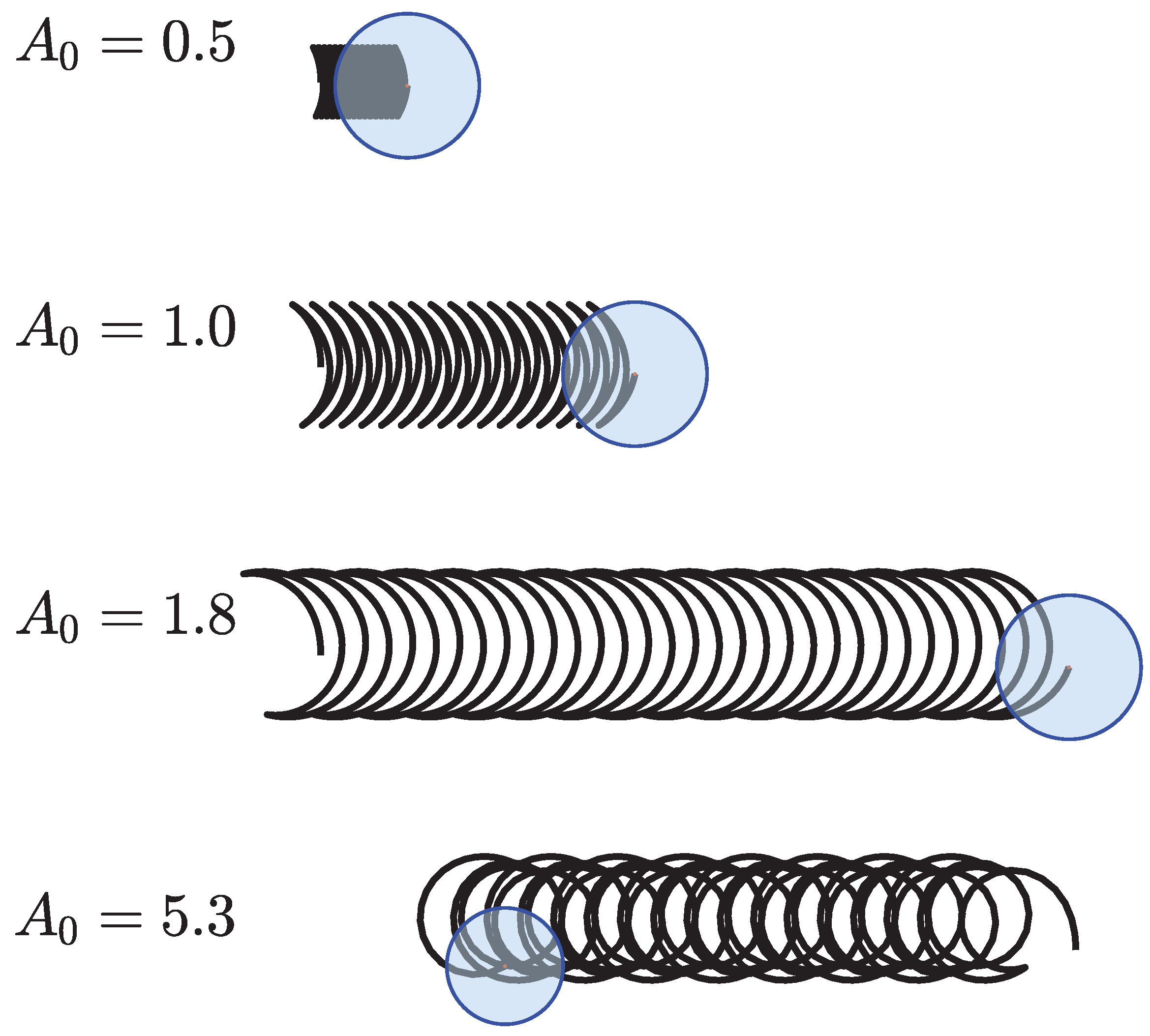
Note that the swimmer can reverse its direction of motion with a large enough ‘shaking’ amplitude. This corresponds to the swimmer shaking hard enough that it completely reverses its direction in one half-period (see Figure 2, bottom). Clearly, this regime is unrealistic, but is interesting to note nonetheless.
7. Efficient Motion
A natural question to ask is: what is the optimal forcing to progress forward as rapidly as possible? This is a popular endeavor in the world of microswimmers; see for instance [9,10,11,12,13,14,15,16,17]. As we see below, we cannot completely answer this question here without some extra assumptions.
7.1. Power
From (15), we can get energy equations
The left-hand sides of (29) are the rate of change of kinetic energy; the right-hand sides include negative quadratic dissipation terms, and power expenditure terms
Averaging (29) gives the balance between power expended and dissipated:
If we use the overdamped approximation (24a) for and the asymptotic solution (21) for , we have
Taking the long-time average yields
For convenience we absorb the prefactor to define
7.2. Optimizing the Speed of Motion
From Equation (25), assuming a periodic forcing ,
where we neglected higher derivatives of A by assuming the period T is long. It is clear from (35) that the power P is an absolute limit to the net speed of motion. A natural question is whether there is an optimal periodic that leads to the fastest speed. For simplicity we take to be an odd function of t, so that in Equation (25). Consider the particular choice of a triangular function
defined on and extended periodically (Figure 4). This piecewise linear function has constant power , so . The speed for this periodic forcing is
where . But now we replace T by a sub-period , and we can see that as . The maximum net speed is thus achieved by a constant-power forcing that ‘switches’ infinitely rapidly with a very small amplitude (Figure 4, bottom). This is not very natural, but still suggests what kinds of motions lead to most efficient propulsion. A follow-up investigation could involve a constraint with a second derivative of A in order to regularize the problem, but this requires introducing additional physics or biology.
8. Discussion
In this paper, we introduced a very simple mechanical model where it’s not initially clear that a swimmer can make forward progress. A mean-zero the forward-backward motion does not lead to net motion, but somewhat surprisingly a sideways motion can do so, as long as it is driven by a force that also exerts a torque. A small amount of rotational inertia is necessary, as is some damping mechanism such as linear drag or friction with a surface. It is likely that the mechanism would still exist in a more realistic model, though this has yet to be verified.
In practice, the forward progress made by the swimmer is extremely slow, so this toy model is probably not a practical means of motion. Nevertheless, it is instructive to explore the full range of possibilities when it comes to self-propelled motion since nature often surprises us. Moreover, the setup described here could probably be easily realized with a simple mechanical robot.
The choice of a disk for the shape is fairly immaterial: the only consequence of the disk shape that was used here is the isotropy of the drag. A nonisotropic drag law (with a resistance matrix) could be used, but would complicate the math. In closing, we note that it is also possible to solve a stochastic version of this problem [18].
Funding
This work was supported by EPSRC grant no EP/R014604/1.
Institutional Review Board Statement
Not applicable.
Informed Consent Statement
Not applicable.
Acknowledgments
The author thanks Jiajia Guo, Giovanni Fantuzzi, and Andrzej Herczynski for helpful discussions. The author also thanks the Isaac Newton Institute for Mathematical Sciences, Cambridge, for support and hospitality during the program Mathematical aspects of turbulence: where do we stand? where work on this paper was completed.
Conflicts of Interest
The author declares no conflict of interest.
References
- Purcell, E.M. Life at low Reynolds number. Am. J. Phys. 1977, 45, 3–11. [Google Scholar] [CrossRef] [Green Version]
- Lauga, E. The Fluid Dynamics of Cell Motility; Cambridge University Press: Cambridge, UK, 2020. [Google Scholar]
- Datt, C.; Nasouri, B.; Elfring, G.J. Two-sphere swimmers in viscoelastic fluids. Phys. Rev. Fluids 2018, 3, 123301. [Google Scholar] [CrossRef] [Green Version]
- Pak, O.S.; Zhu, L.; Brandt, L.; Lauga, E. Micropropulsion and microrheology in complex fluids via symmetry breaking. Phys. Fluids 2012, 24, 103102. [Google Scholar] [CrossRef] [Green Version]
- Zhu, L.; Lauga, E.; Brandt, L. Self-propulsion in viscoelastic fluids: Pushers vs. pullers. Phys. Fluids 2012, 24, 051902. [Google Scholar] [CrossRef] [Green Version]
- Klotsa, D.; Baldwin, K.A.; Hill, R.J.; Bowley, R.M.; Swift, M.R. Propulsion of a two-sphere swimmer. Phys. Rev. Lett. 2015, 115, 248102. [Google Scholar] [CrossRef] [PubMed] [Green Version]
- Bocquet, L.; Piasecki, J. Microscopic derivation of non-Markovian thermalization of a Brownian particle. J. Stat. Phys. 1997, 87, 1005–1035. [Google Scholar] [CrossRef] [Green Version]
- Hinch, E.J. Application of the Langevin equation to fluid suspensions. J. Fluid Mech. 1975, 72, 499. [Google Scholar] [CrossRef] [Green Version]
- Childress, S. Mechanics of Swimming and Flying; Cambridge University Press: Cambridge, UK, 1981. [Google Scholar]
- Gueron, S.; Levit-Gurevich, K. Energetic considerations of ciliary beating and the advantage of metachronal coordination. Proc. Natl. Acad. Sci. USA 1999, 96, 12240–12245. [Google Scholar] [CrossRef] [PubMed] [Green Version]
- Lauga, E.; Powers, T.R. The hydrodynamics of swimming micro-organisms. Rep. Prog. Phys. 2009, 72, 096601. [Google Scholar] [CrossRef]
- Michelin, S.; Lauga, E. Efficiency optimization and symmetry-breaking in a model of ciliary locomotion. Phys. Fluids 2010, 22, 111901. [Google Scholar] [CrossRef] [Green Version]
- Michelin, S.; Lauga, E. Optimal feeding is optimal swimming for all Péclet numbers. Phys. Fluids 2011, 23, 101901. [Google Scholar] [CrossRef] [Green Version]
- Michelin, S.; Lauga, E. Unsteady feeding and optimal strokes of model ciliates. J. Fluid Mech. 2013, 715, 1–31. [Google Scholar] [CrossRef] [Green Version]
- Pironneau, O.; Katz, D.F. Optimal swimming of flagellated micro-organisms. J. Fluid Mech. 1974, 66, 391–415. [Google Scholar] [CrossRef]
- Spagnolie, S.E.; Lauga, E. The optimal elastic flagellum. Phys. Fluids 2010, 22, 031901. [Google Scholar] [CrossRef] [Green Version]
- Tam, D.; Hosoi, A.E. Optimal stroke patterns for Purcell’s three-link swimmer. Phys. Rev. Lett. 2007, 98, 068105. [Google Scholar] [CrossRef] [PubMed] [Green Version]
- Thiffeault, J.-L.; Guo, J. Shake your hips: An anisotropic active Brownian particle with a fluctuating propulsion force. arXiv 2021, arXiv:2102.11758. [Google Scholar]
Figure 1.
Disk of radius a with a force acting at a distance ℓ from its geometric center.

Figure 2.
Trajectories for and , .

Figure 3.
The mean speed U for numerical simulations with , (solid line) and the asymptotic form Equation (27).
Figure 3.
The mean speed U for numerical simulations with , (solid line) and the asymptotic form Equation (27).

Figure 4.
Top: The periodically-extended triangular function (36) for . Bottom: The same function with T replaced by . The two functions have the same constant power , but the bottom function has smaller amplitude.
Figure 4.
Top: The periodically-extended triangular function (36) for . Bottom: The same function with T replaced by . The two functions have the same constant power , but the bottom function has smaller amplitude.

Publisher’s Note: MDPI stays neutral with regard to jurisdictional claims in published maps and institutional affiliations. |
© 2022 by the author. Licensee MDPI, Basel, Switzerland. This article is an open access article distributed under the terms and conditions of the Creative Commons Attribution (CC BY) license (https://creativecommons.org/licenses/by/4.0/).
Share and Cite
MDPI and ACS Style
Thiffeault, J.-L. Moving Forward by Shaking Sideways. Symmetry 2022, 14, 620. https://0-doi-org.brum.beds.ac.uk/10.3390/sym14030620
AMA Style
Thiffeault J-L. Moving Forward by Shaking Sideways. Symmetry. 2022; 14(3):620. https://0-doi-org.brum.beds.ac.uk/10.3390/sym14030620
Chicago/Turabian StyleThiffeault, Jean-Luc. 2022. "Moving Forward by Shaking Sideways" Symmetry 14, no. 3: 620. https://0-doi-org.brum.beds.ac.uk/10.3390/sym14030620
Note that from the first issue of 2016, this journal uses article numbers instead of page numbers. See further details here.