Symmetry and Asymmetry in the Fluid Mechanical Sewing Machine

Abstract

The ‘fluid mechanical sewing machine’ is a device in which a thin thread of viscous fluid falls onto a horizontal belt moving in its own plane, creating a rich variety of ‘stitch’ patterns depending on the fall height and the belt speed. This review article surveys the complex phenomenology of the patterns, their symmetries, and the mathematical models that have been used to understand them. The various patterns obey different symmetries that include (slightly imperfect) fore–aft symmetry relative to the direction of belt motion and invariance under reflection across a vertical plane containing the velocity vector of the belt, followed by a shift of one-half the wavelength. As the belt speed decreases, the first (Hopf) bifurcation is to a ‘meandering’ state whose frequency is equal to the frequency ${\Omega }_c$ of steady coiling on a motionless surface. More complex patterns can be studied using direct numerical simulation via a novel ‘discrete viscous threads’ algorithm that yields the Fourier spectra of the longitudinal and transverse components of the motion of the contact point of the thread with the belt. The most intriguing case is the ‘alternating loops’ pattern, the spectra of which are dominated by the first five multiples of ${\Omega }_c/3$. A reduced (three-degrees-of-freedom) model succeeds in predicting the sequence of patterns observed as the belt speed decreases for relatively low fall heights for which inertia in the thread is negligible. Patterns that appear at greater fall heights seem to owe their existence to weakly nonlinear interaction between different ‘distributed pendulum’ modes of the quasi-vertical ‘tail’ of the thread.

1. Introduction

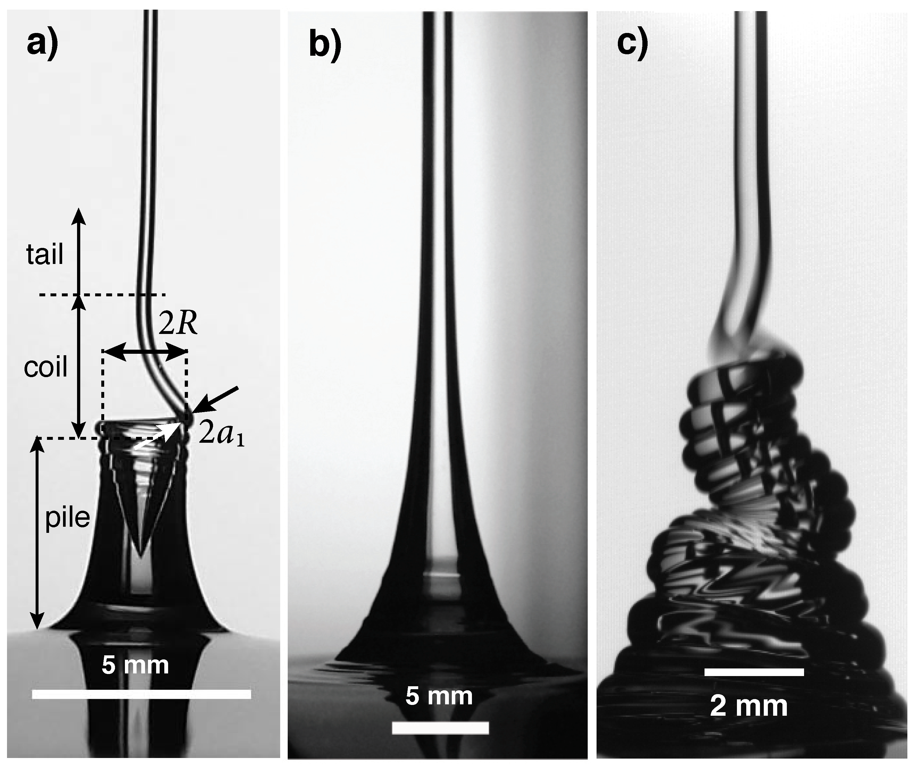
Everyone is familiar with the beautiful ‘liquid thread coiling’ instability (also known as ‘liquid rope coiling’) that occurs when a thin stream of honey falls onto a piece of toast (Figure 1a). Liquid coiling is a classic example of a symmetry-breaking bifurcation. In this case, the basic state is an axisymmetric stagnation flow (Figure 1b). When the fall height H exceeds a critical value (for small heights) or the volumetric flow rate Q becomes less than a critical value (for large heights), the stagnation flow becomes unstable to small lateral perturbations (incipient bending) of the thread’s axis. The instability eventually saturates to form a coil with a finite radius R that rotates about the vertical with an angular frequency $\Omega$. The resulting structure comprises three distinct parts in general: an upper quasi-vertical ‘tail’, the ‘coil’ in which the thread is strongly bent, and an underlying ‘pile’ of fluid previously laid down by the coiling. The essential difference between the tail and the coil is that deformation of the former is dominated by stretching, whereas the deformation of the coil is dominated by bending. Since the equations that describe bending are of higher order in the arcwise derivatives than those describing stretching, the coil can be thought of as a boundary layer that ensures the satisfaction of all the relevant boundary conditions at the contact point with the pile.

In laboratory experiments, the formation of a pile on the surface is unavoidable. Under some conditions, this pile is a steady-state feature (Figure 1a), while under others it is itself unstable to small perturbations, leading to periodic collapse or quasi-steady secondary buckling (Figure 1c). Especially in these latter cases, the time-dependence of the pile corresponds to a rather ‘dirty’ unsteady boundary condition at the bottom of the freely coiling thread. It is thus natural to ask: what would happen if we could continuously remove all the fluid laid down by the coiling, thereby doing away with the pile? An easy way to do this comes to mind: it is to let the fluid fall, not onto a motionless surface, but onto a surface moving with a constant horizontal speed V. The result is the “fluid mechanical sewing machine” (FMSM), a name first coined by Chiu-Webster and Lister [1].

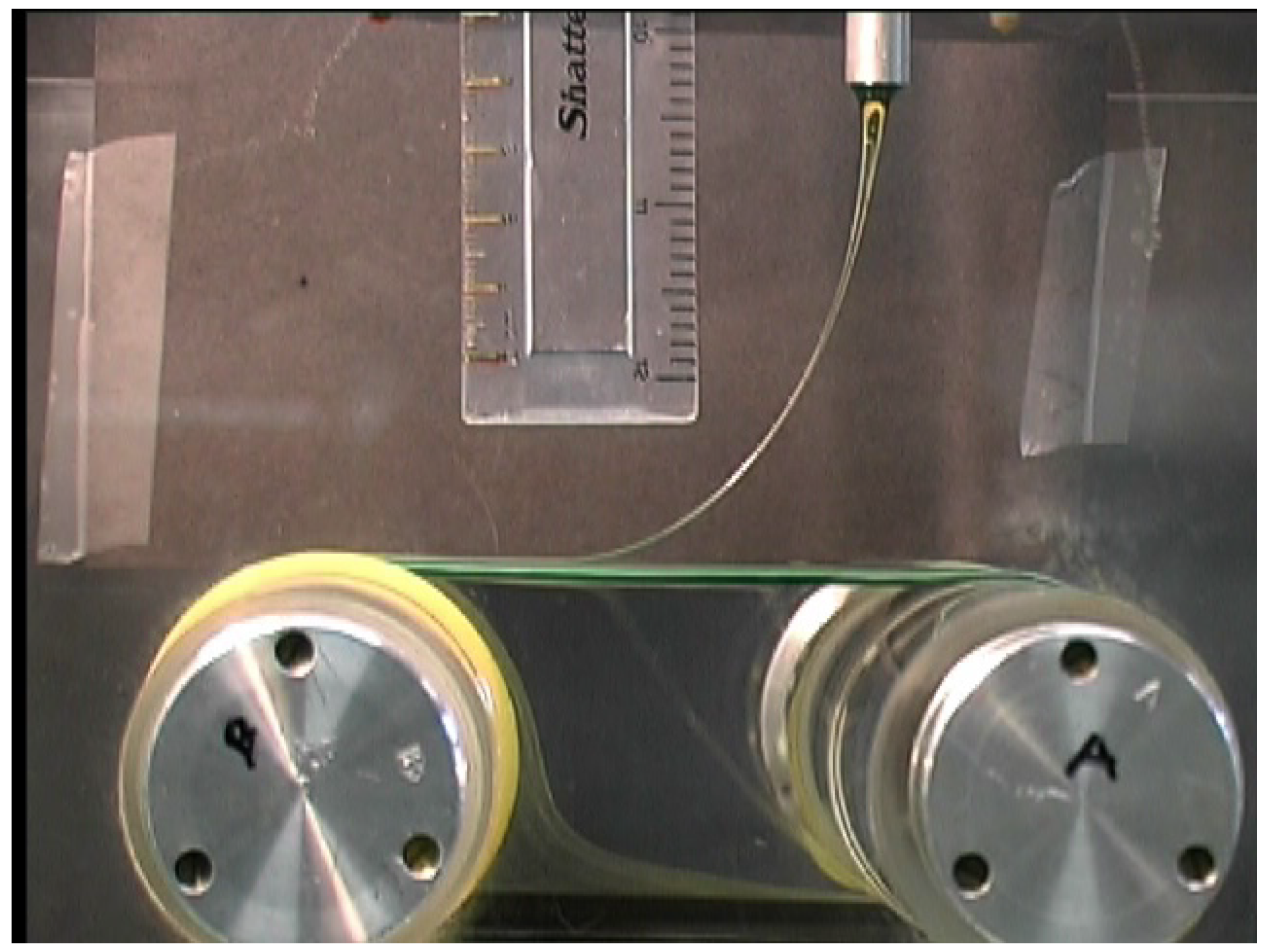
Figure 2 shows a simple laboratory apparatus that realizes the FMSM. A fluid thread ejected at a constant volumetric rate Q from a nozzle falls onto a belt in the form of a closed loop that is kept in motion by two rollers. When V is sufficiently high, the thread is stretched in the downstream direction and remains confined to a vertical plane, as shown in Figure 2. However, when V is less than a critical value, the thread becomes unstable to out-of-plane oscillations. This oscillatory motion leaves complex traces of fluid on the belt that resemble stitch patterns when viewed from above, hence the name FMSM.

The first investigations of the dynamics of threads of viscous fluid falling onto surfaces were the experimental studies of liquid thread coiling by G. Barnes and collaborators [2,3]. Since then, liquid thread coiling has been studied in depth using laboratory experiments [4,5,6,7,8,9,10,11,12,13,14] linear stability analysis [11,15,16], scaling analysis [8], asymptotic analysis [17], and numerical analysis based on slender-thread theory [9,10,11,12,13,14,18]. Interest in the more complicated case of a moving surface—the FMSM—began with the pioneering study of Chiu-Webster and Lister [1], who performed laboratory experiments and proposed a theoretical model in which the thread deforms by stretching alone, without bending. In the same year, Ribe et al. [19] proposed a theoretical model that included bending. They performed a linear stability analysis of the steady dragged state of the thread, and found that the predicted critical belt speed and frequency for the onset of out-of-plane oscillations (meandering) agreed closely with the experimental measurements of [1]. Extensive laboratory experiments with improved apparatus were performed by Morris et al. [20], who determined a detailed phase diagram of the stitch patterns as a function of fall height and belt speed. They showed that the onset of meandering is a Hopf bifurcation, and applied equivariant bifurcation theory together with symmetry constraints to determine generic amplitude equations for interacting modes of the thread’s motion. Blount and Lister [21] used matched asymptotic expansions to determine the structure and stability of a dragged viscous thread in the limit of extreme slenderness. Brun et al. [22] performed numerical simulations of the FMSM patterns using an algorithm based on a discrete formulation of the slender-thread equations, and classified the different patterns according to their Fourier spectra. Finally, Brun et al. [23] proposed a reduced (three-degrees-of-freedom) model for non-inertial FMSM patterns, and showed that the model equations accurately predict the sequence of bifurcations that occur as the belt speed changes.

This review article begins in Section 2 by surveying the complex phenomenology of the stitch patterns and classifying them according to their symmetries. Section 3 reviews liquid thread coiling on a motionless surface, the physics of which underlies the FMSM. Section 4 examines the initial bifurcation from a steady dragged thread to meandering via a linear stability analysis based on the theory of slender viscous threads. Section 5 presents direct numerical simulations of the stitch patterns using a ‘discrete viscous threads’ (DVT) numerical model. Section 6 presents a spectral analysis of selected stitch patterns based on DVT simulations. Section 7 discusses a reduced model for inertia-free stitch patterns that explains several curious features of the more complicated DVT simulations. Finally, Section 8 discusses the (slightly imperfect) fore–aft symmetry of many of the patterns, and closes with some suggestions for further research.

2. Stitch Patterns

Figure 3 shows an essentially complete catalog of the stitch patterns observed experimentally in the FMSM. In this preliminary presentation, the patterns are shown ‘all in a jumble’, with no attempt to indicate the relationships between them. Apart from the disordered pattern and the steady dragged thread, all the other patterns are periodic in the coordinate x parallel to the belt’s motion, with a well-defined primary wavelength $\lambda$.

It is instructive to classify the patterns by their different symmetries. Let y be the horizontal coordinate normal to the direction of the belt’s motion, with origin on the line below the center of the nozzle. Because not all patterns are graphs $y\left(x\right)$, we describe each pattern by the pair of functions $x\left(s\right)$, $y\left(s\right)$, where s is the arclength along the thread’s axis. Let ${\lambda }_s$ be the ‘arcwise wavelength’, i.e., the total arclength of the thread contained within one wavelength $\lambda$ in the x-direction.

Table 1. Symmetries of stitch patterns observed experimentally. An X indicates a pattern having the symmetry shown at the top of each column.

Pattern	$\mathit{y}\left(\mathit{s}\right)=0$	$\mathit{y}(\mathit{s}+{\mathit{\lambda }}_{\mathit{s}}/2)=-\mathit{y}\left(\mathit{s}\right)$	$\mathit{y}({\mathit{s}}_0-\mathit{s})=\mathit{y}\left(\mathit{s}\right)$	$\mathit{y}(\mathit{s}+{\mathit{\lambda }}_{\mathit{s}})=\mathit{y}\left(\mathit{s}\right)$
Flat (dragged thread)	X	X	X	X
Meanders	−	X	X	X
Alternating loops	−	X	X	X
Two-by-two	−	X	X	X
Translated coiling	−	−	X	X
W pattern	−	−	X	X
Bunched meanders	−	−	−	X
Braiding	−	−	−	X
Bunched double coiling	−	−	−	X
Slanted loops	−	−	−	X
Double meanders	−	−	−	X
Sidekicks	−	−	−	X
Disordered	−	−	−	−

shows the symmetries of the patterns. The most highly symmetric pattern is of course the steady dragged thread with $y\left(s\right)=0$, which exhibits (trivial) mirror symmetry across the vertical plane $y=0$. Among the periodic patterns, three (meanders, alternating loops, and two-by-two) have the symmetry $y(s+{\lambda }_s/2)=-y\left(s\right)$. This corresponds to reflecting the pattern across the line $y=0$ and then shifting it longitudinally by an amount ${\lambda }_s/2$. Next comes the symmetry $y(s_0-s)=y\left(s\right)$ for some $s_0$, which corresponds to fore–aft symmetry with respect to the direction of belt motion. In addition to the patterns already mentioned, translated coiling and the W-pattern exhibit this symmetry. Finally, the lowest symmetry is simple periodicity such that $y(s+{\lambda }_s)=y\left(s\right)$. All the patterns except the disordered one are periodic.

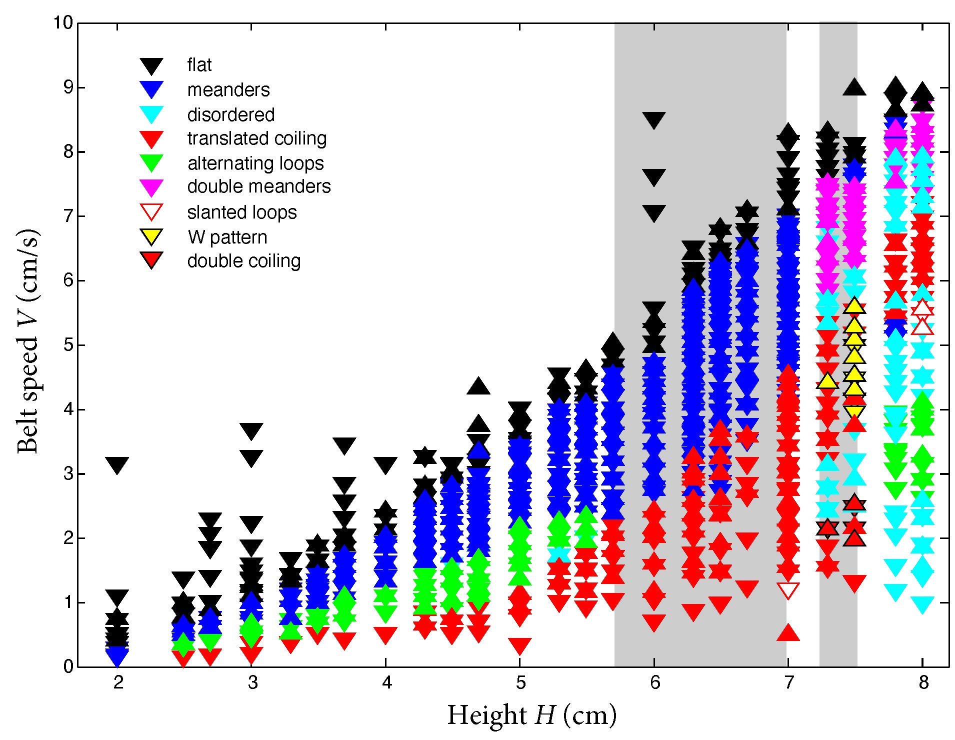
To understand better the relationships among the patterns, it is helpful to examine a phase diagram showing where each pattern is observed in the space of belt speed and fall height. Figure 4 shows such a diagram for the values of the viscosity $\nu$ and the flow rate Q given in the caption. For fall heights $H\le 5.5$ cm, the patterns appear in the order flat - meanders - alternating loops - translated coiling as the belt speed decreases. For greater fall heights, alternating loops disappear, only to reappear again around $H=7.8$ cm. The phase diagram is particularly rich for $H\ge 7.2$ cm, where additional patterns such as the W-pattern, double coiling, biperiodic meanders, and slanted loops are seen. Much of the region $H\ge 7.2$ cm is given over to disordered patterns, which occur in ‘patches’ in the H-V space bounded by regions of periodic patterns.

3. Basics of Liquid Thread Coiling

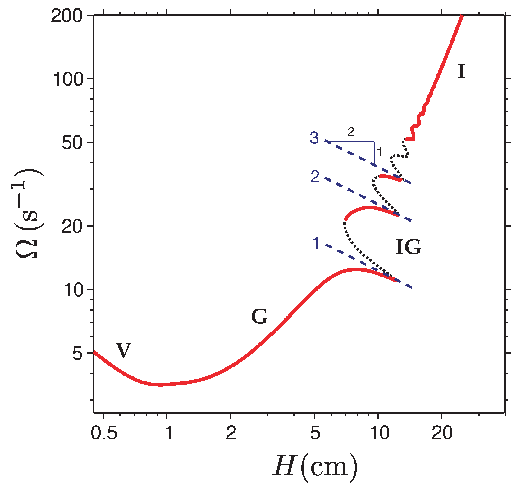
As the dynamics of liquid thread coiling underly those of the FMSM, it is important to start by developing a basic understanding of the former. Liquid thread coiling can best be understood by considering how its angular frequency $\Omega$ depends on the fall height H, which is the main control parameter. Figure 5 shows a typical variation of $\Omega$ as a function of H. As H increases, the relative importance of the viscous, gravitational, and inertial forces acting on the coiled portion of the thread changes, leading to four distinct regimes of liquid thread coiling. At very low fall heights, both gravity and inertia are negligible compared to viscous forces. The coiling in this ‘viscous’ (V) regime is purely kinematic, driven by the forced extrusion of the fluid from a nozzle, and the coiling frequency scales as [18]

$${\Omega }_V\sim \frac{U_1}{H}$$

(1)

where $U_1=Q/\left(\pi a_1^2\right)$ is the typical axial velocity of the fluid and $a_1$ is (to recall) the thread radius at the top of the pile. At somewhat larger fall heights, the viscous forces are balanced by gravity while inertia remains negligible. In this ‘gravitational’ (G) regime, the coiling frequency scales as [17]

$${\Omega }_G\sim \frac{U_1}{\delta }{\left(ln\frac{H}{\delta }\right)}^{-1/2}$$

(2)

where $\delta \sim {\left(\nu Q/g\right)}^{1/4}$ is the length scale over which gravity balances viscous forces in the coil and $\nu$ is the kinematic viscosity. The logarithmic term appears because the tail behaves like a catenary, which is deflected by an amount $\propto F|lnF|$ by a horizontal force F associated with bending in the coil. At very large fall heights, the dominant forces in the coil are viscous forces and inertia. This is the ‘inertial’ (I) regime, in which $\Omega$ scales as [8]

$${\Omega }_I\sim {\left(\frac{Q^4}{\nu a_1^{10}}\right)}^{\frac{1}{3}}$$

(3)

At fall heights intermediate between the G and I regimes, there appears an ‘inertio-gravitational’ (IG) regime in which $\Omega$ is a multivalued function of H. In this regime the tail of the thread behaves as a distributed pendulum that enters into resonance with the coil whenever the frequency ${\Omega }_G$ fixed by the coil is close to one of the natural oscillation frequencies of the tail. These frequencies are [10]

$${\Omega }^{\left(n\right)}=C_n{\left(\frac{g}{H}\right)}^{1/2},n=1,2,...$$

(4)

where $C_n$ are constants of proportionality. The coiling frequency ${\Omega }_{IG}\left(H\right)$ in this regime defines a set of resonance peaks centered on lines with slope $-1/2$ on a log–log plot of $\Omega$ vs. H (Figure 5).

Finally, the relation between $a_1$ and H depends on the dimensionless fall height $\widehat{H}\equiv H{(g/{\nu }^2)}^{1/3}$. For $\widehat{H}<2$, the weight of the fluid in the tail is balanced primarily by the viscous resistance to stretching, and $a_1\sim {(\nu Q/g{H}^2)}^{1/2}$. For $\widehat{H}>10$, the weight is balanced primarily by the vertical momentum flux, and $a_1\sim {(Q^2/gH)}^{1/4}$.

4. Onset of Meandering

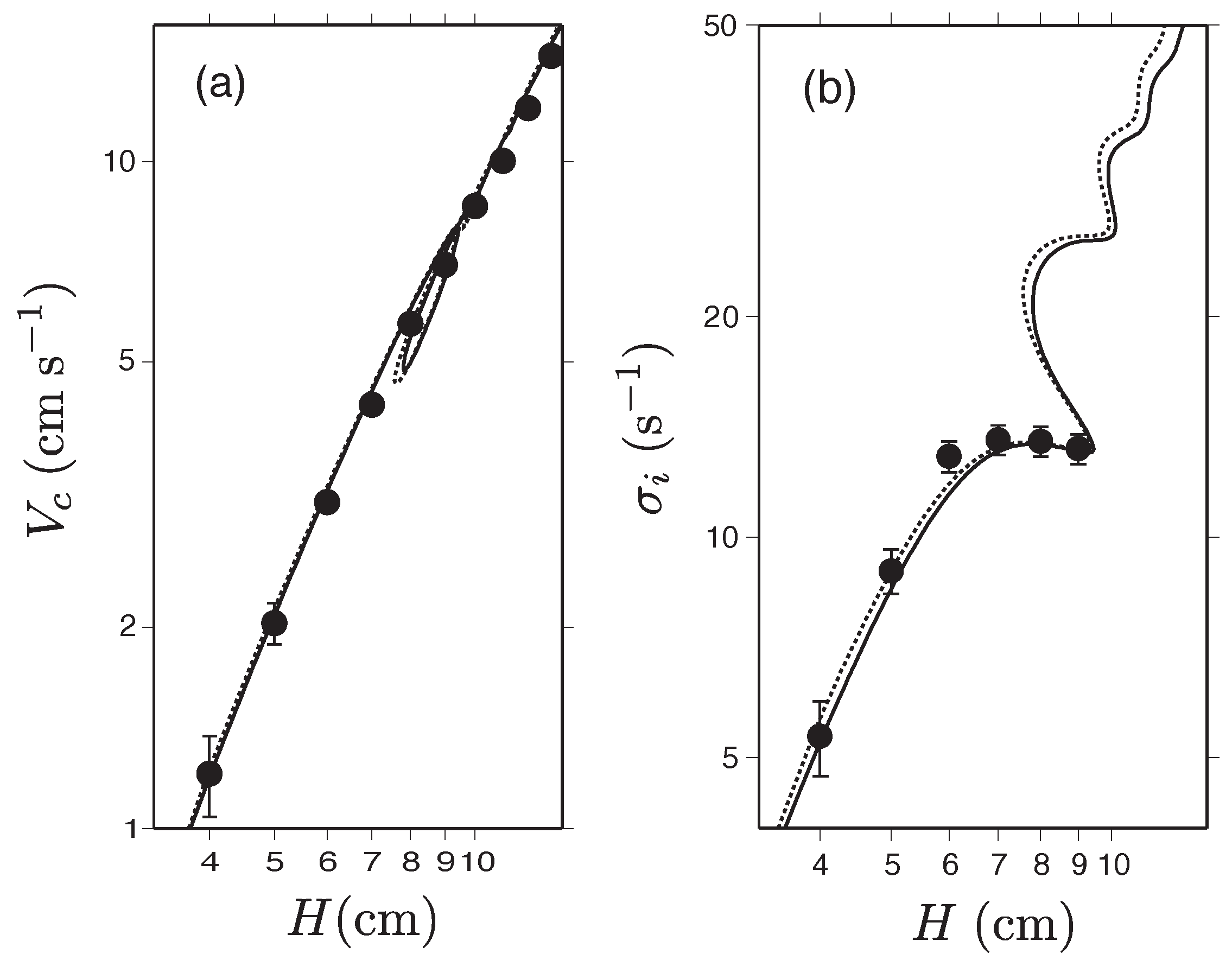
We now examine more closely the first bifurcation in the FMSM from a steady dragged thread to meandering. This bifurcation was studied experimentally by Chiu-Webster and Lister [1] and Morris et al. [20], and theoretically by Ribe et al. [19], Morris et al. [20], and Blount and Lister [21]. Figure 6a compares experimental measurements (circles) of the critical belt speed $V_c$ [1] with the prediction (solid line) of a numerical linear stability analysis of the equations governing the motion of a slender viscous thread with inertia deforming by stretching, bending, and twisting [19]. The parameters of the experiment are given in the figure caption. The experiments and the numerics agree remarkably well.

To understand the origin of the critical belt speed, it is revealing to compare the quantity $V_c$ with the vertical speed $U_1\equiv Q/\left(\pi a_1^2\right)$ of a coiling viscous thread that has fallen through a distance H onto a stationary surface. The function $U_1\left(H\right)$, calculated numerically using the method of Ribe [18] for the parameters of the FMSM experiment in question, is shown by the dashed line in Figure 6a. The solid and dashed lines are nearly indistinguishable, indicating that $V_c=U_1$ with negligible error. This result has a simple kinematical interpretation: meandering begins when the belt speed becomes too slow to advect away in a straight line the fluid falling onto it.

Further insight can be obtained by comparing the angular frequency ${\sigma }_i$ of incipient meandering (i.e., the imaginary part of the growth rate predicted by linear stability analysis) with the angular frequency $\Omega$ of liquid thread coiling with the same parameters. These two quantities are shown as functions of H by solid and dashed lines in Figure 6b, respectively. The two curves track each other closely apart from a small systematic offset. This means that for a given fall height the frequency of incipient meandering is nearly equal to the frequency of liquid thread coiling on a motionless surface.

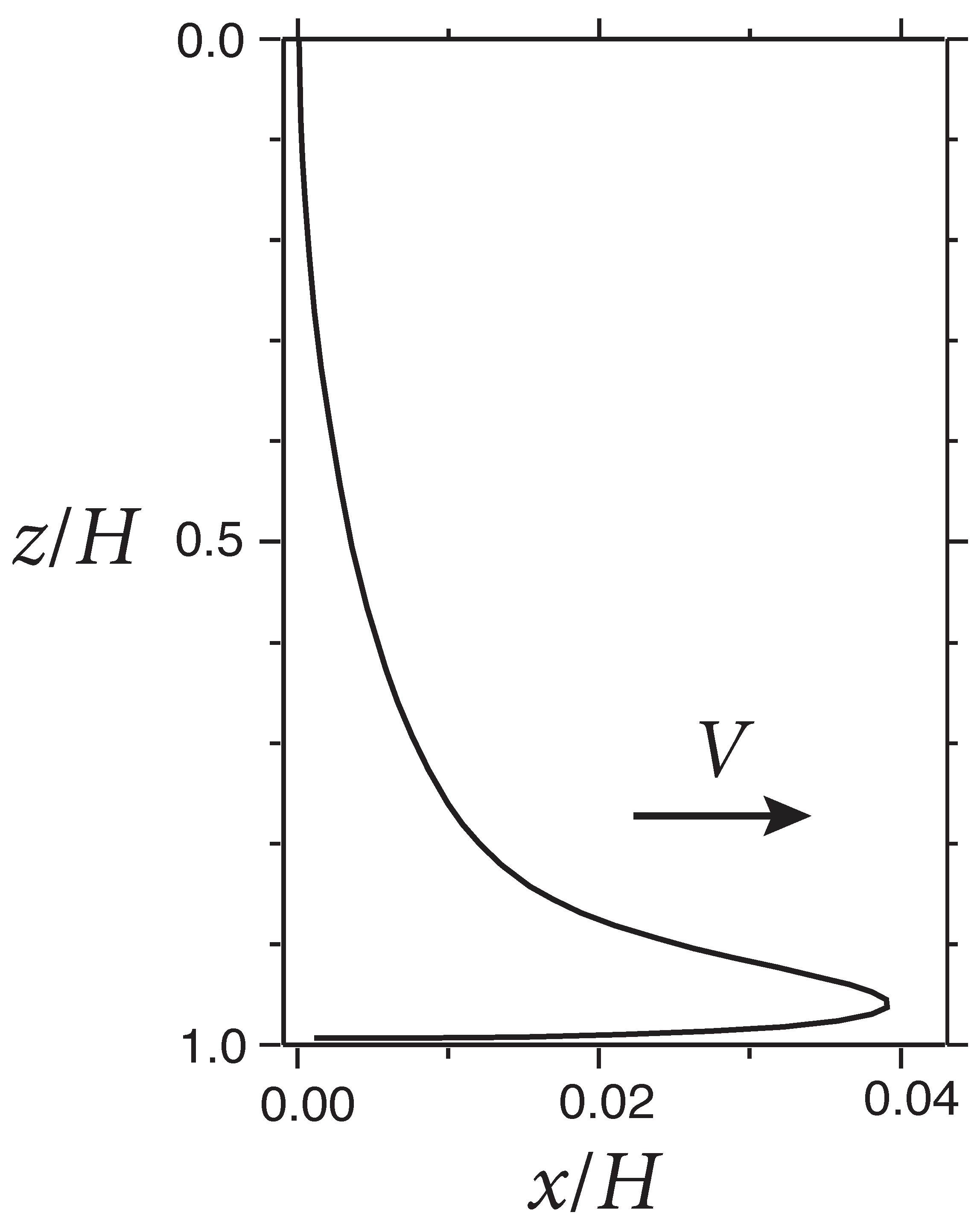
Deeper physical insight into the mechanism of incipient meandering is provided by the asymptotic stability analysis of Blount and Lister [21]. These authors focus on the ‘gravitational heel’ structure of the lowermost part of the thread when $V\approx U_1$. The shape of this heel (Figure 7) results from a steady balance of the weight of the fluid and the viscous forces that resist bending of the thread. The asymptotic analysis shows that the thread is stable to meandering if bending forces in the heel pull the tail in the same direction as the belt motion, and unstable if the tail is pushed against the belt motion. Blount and Lister [21] liken the latter situation to the heel ‘losing its balance’.

The linear stability analyses discussed above are limited to meandering of infinitesimal amplitude. Finite-amplitude meandering was studied by Morris et al. [20] using a phenomenological model in which the amplitude A of the meandering is governed by a Landau equation

$$\tau \dot{A}=ϵA-\mu A{\left|A\right|}^2+\mathrm{h}.\mathrm{o}.\mathrm{t}.$$

(5)

where $ϵ=(V_c-V)/V_c$ is the degree of supercriticality, $\tau$ is a time scale related to the linear growth rate of the instability, and h.o.t. denotes higher-order terms. For small amplitudes $A\ll 1$, we can write down perturbation expansions for the position $\left(x\right(t),y(t\left)\right)$ of the contact point. Now the reflectional symmetry of the catenary implies that the out-of-plane variable $y\left(t\right)$ must be an odd function of A, while the in-plane variable $x\left(t\right)$ must be an even function of A. Thus the position of the contact point must have the form

$$y\left(t\right)=Asin\omega t+O\left(A^3\right),$$

(6)

$$x\left(t\right)=x_0+Bcos(2\omega t+\varphi )+O\left(A^4\right)$$

(7)

where $B=O\left(A^2\right)$, $\omega ={\omega }_c+O\left(A^2\right)$, ${\omega }_c$ is the frequency of the onset of meandering, $\varphi$ is a constant phase, and $x_0$ is the unperturbed displacement to within an $O\left(A^2\right)$ correction. The absolute speed $W\left(t\right)$ of the contact point is

$$W^2={(\dot{x}-V)}^2+{\dot{y}}^2=V^2+4B\omega Vsin(2\omega t+\varphi )+\frac{A^2{\omega }^2}{2}(1+cos2\omega t)+O\left(A^4\right).$$

(8)

We now assume that W is constant and equal to the free-fall speed $U_1$, which is in turn equal to the critical belt speed $V_c$. Setting $W=V_c$ in (8), we find

$$V_c^2=V^2+\frac{A^2{\omega }^2}{2}+O\left(A^4\right),$$

(9)

$$B=\frac{A^2\omega }{8V}+O\left(A^4\right),\varphi =\frac{\pi }{2}+O\left(A^2\right).$$

(10)

Rearranging (9), we obtain

$$A^2=\frac{2(V_c^2-V^2)}{{\omega }^2}\approx \frac{4V_c^2}{{\omega }_c^2}\frac{V_c-V}{V_c},$$

(11)

which when compared with the steady form of (5) gives

$$\mu ={({\omega }_c/2V_c)}^2.$$

(12)

This generic argument yields the amplitude of the meanders close to threshold. Morris et al. [20] showed in their Figure 8 that the kinematic estimate (12) agreed closely with experimental measurements for fall heights $H>5.5$ cm.

5. Direct Numerical Simulation

Brun et al. [22] performed a direct numerical simulation of the FMSM using a ‘discrete viscous threads’ (DVT) algorithm that is most fully discussed in Audoly et al. [24]. Such simulations allow one rapidly to construct a phase diagram of the FMSM patterns by varying adiabatically the fall height H and the belt speed V. Brun et al. [22] presented their phase diagrams in the space of dimensionless fall height $\widehat{H}$ and belt speed $\widehat{V}$ defined by

$$\widehat{H}=H{\left(\frac{g}{{\nu }^2}\right)}^{1/3},\widehat{V}=V{\left(\nu g\right)}^{-1/3}.$$

(13)

A given phase diagram is uniquely identified by the values of the following three dimensionless groups that are independent of both H and V:

$${\Pi }_1={\left(\frac{{\nu }^5}{g{Q}^3}\right)}^{1/5},{\Pi }_2={\left(\frac{\nu Q}{g{d}^4}\right)}^{1/4},{\Pi }_3=\frac{\gamma d^2}{\rho \nu Q}.$$

(14)

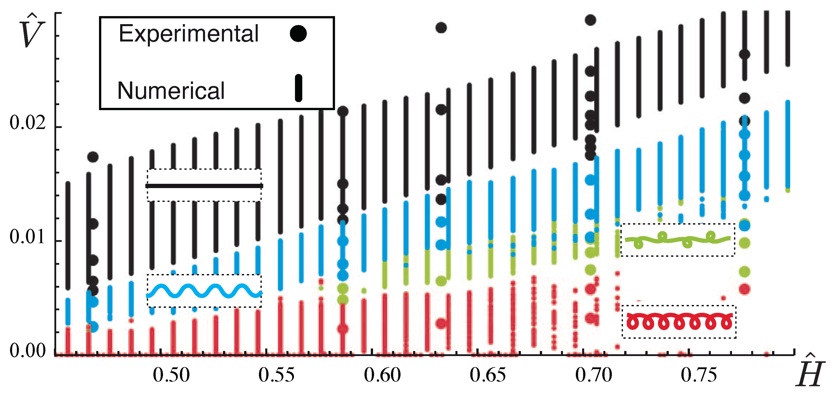
Figure 8 shows the phase diagram predicted using DVT for ${\Pi }_1=670$, ${\Pi }_2=0.37$, and ${\Pi }_3=1.84$ (vertical lines), together with experimental data from Morris et al. [20] for the same parameters (circles). The fall heights $\widehat{H}\le 0.8$ here are ‘low’ values in the sense that inertia is negligible throughout the thread. The agreement between the numerics and the experiments is quite good, although a tendency for the predicted boundaries to be slightly higher than the experimental ones is noticeable.

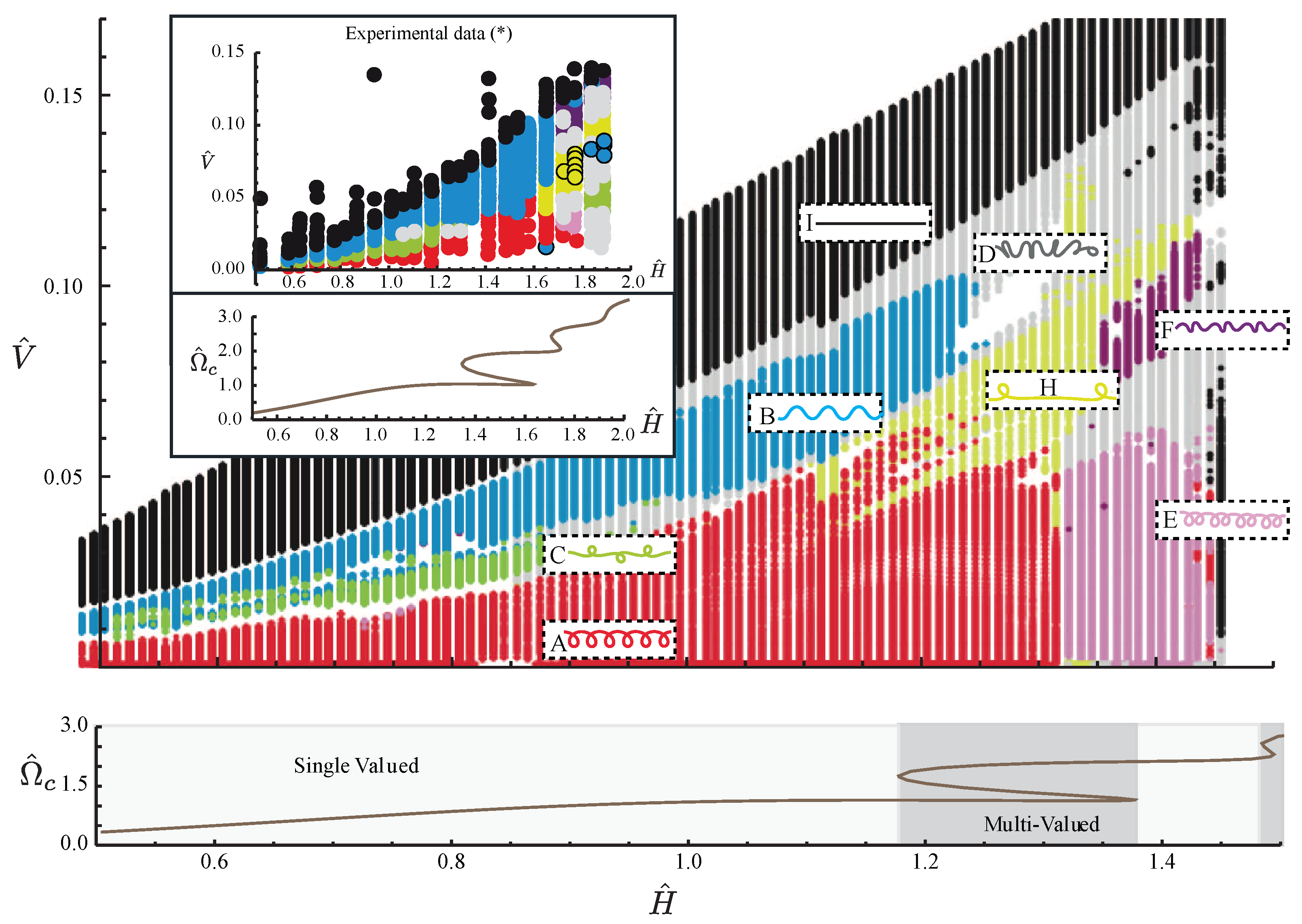
For fall heights $\widehat{H}>0.8$, Brun et al. [22] encountered numerical difficulties if surface tension was present (${\Pi }_3>0$). Accordingly, they assumed ${\Pi }_3=0$ in order to be able to construct a phase diagram for $\widehat{H}$ up to 1.5. Figure 9 compares this phase diagram (main portion) with the experimentally determined phase diagram for the same values of ${\Pi }_1$ and ${\Pi }_2$, but ${\Pi }_3=1.84$ (inset). The topology of the two diagrams is broadly similar. Nevertheless, it should be noted that the maximum values of $\widehat{H}$ in the two diagrams are different, such that a given pattern appears at larger values of $\widehat{H}$ in the laboratory (where surface tension is unavoidable) than in the numerics with ${\Pi }_3=0$. There are also a number of significant differences in detail. In particuliar, the W, slanted loop, and alternating loop patterns are observed in the experiments for $\widehat{H}>1.7$, but do not occur in the high-$\widehat{H}$ portion of the numerical phase diagram.

6. Spectral Analysis of the Patterns

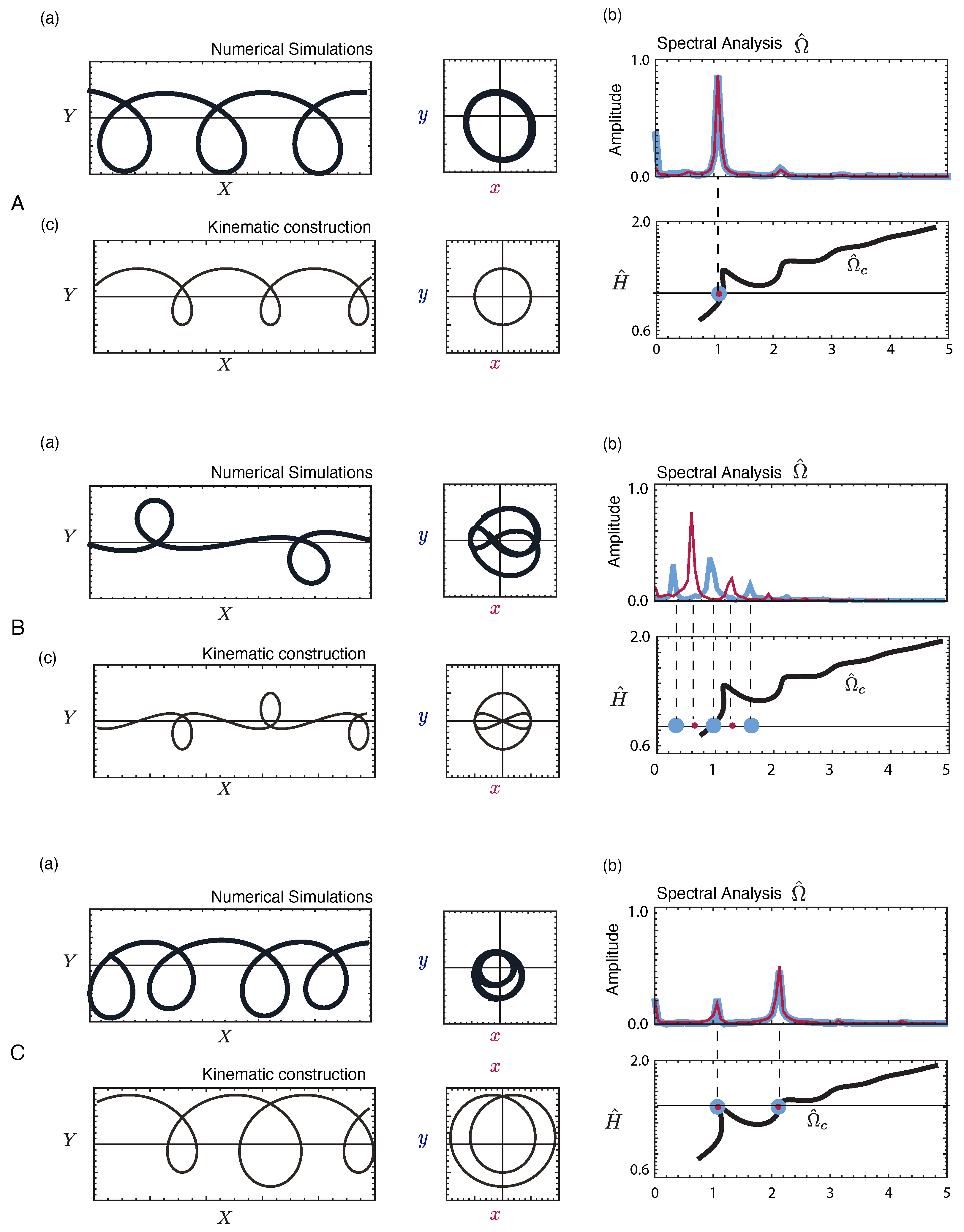
A revealing way to characterize the different FMSM patterns is to calculate the Fourier spectra of the time-varying longitudinal coordinate $x\left(t\right)$ and transverse coordinate $y\left(t\right)$ of the contact point of the thread with the belt. Figure 10 illustrates the spectral characteristics of three FMSM patterns: translated coiling (A), alternating loops (B), and double coiling (C). In each of the three panels, part (a) shows the trace on the belt calculated using DVT (left) and the trajectory of the contact point in the frame of the nozzle (right). Part (b), ‘Spectral analysis’, shows the Fourier transforms of the longitudinal (red) and transverse (blue) motion of the contact point (top), together with the corresponding steady coiling frequency $\widehat{\Omega }(\widehat{H})$ (bottom). Translated coiling, the simplest of the three patterns, is characterized by a quasi-circular movement of the contact point around the center of the nozzle. Both the longitudinal and transverse motions are dominated by the same single frequency, which is close to the steady coiling frequency for the height in question ($\widehat{H}\approx 1.3$). Turning to the more complicated alternating loops pattern, we see that the longitudinal and transverse spectra are now dominated by different frequencies, with five distinct peaks in total. The largest peak occurs for longitudinal motion, with a frequency locked to the value $2{\Omega }_c/3$. There is also a secondary peak at $4{\Omega }_c/3$. The transverse motion on the other hand has dominant frequencies ${\Omega }_c/3$, ${\Omega }_c$, and $5{\Omega }_c/3$. Finally, for the double coiling pattern both the longitudinal and transverse motions are dominated by the same two frequencies in the ratio 2:1. These frequencies are very close to the two steady coiling frequencies that coexist at the height in question ($\widehat{H}\approx 1.42$).

As a final step in our analysis, we reconstruct the patterns by summing the first few terms in a Fourier expansion of the form

$$x\left(t\right)+iy\left(t\right)=\sum _{j=1}^{N_x}{\alpha }_{j}cos({\omega }_j^{x}t+{\varphi }_j^x)+i\sum _{j=1}^{N_y}{\beta }_{j}cos({\omega }_j^{y}t+{\varphi }_j^y).$$

(15)

where $i=\sqrt{-1}$. In (15), ${\omega }_j^x$, ${\varphi }_j^x$, and ${\alpha }_j$ are the angular frequency, phase, and amplitude of mode j of the longitudinal motion of the contact point, while ${\omega }_j^y$, ${\varphi }_j^y$, and ${\beta }_j$ are the analogous quantities for the transverse motion. It turns out that all the patterns can be reconstructed accurately by retaining at most two frequencies in each direction, i.e., $N_x\le 2$ and $N_y\le 2$.

Table 2. Spectral characteristics of several FMSM patterns. The parameters shown are those that appear in the kinematic model (15). The frequency 1 is assigned to the peak in the spectrum with the largest amplitude. A star indicates a frequency that is locked to the steady coiling frequency ${\widehat{\Omega }}_c$.

Pattern	${\mathit{\omega }}_1^{\mathit{x}}$	${\mathit{\omega }}_2^{\mathit{x}}$	${\mathit{\omega }}_1^{\mathit{y}}$	${\mathit{\omega }}_2^{\mathit{y}}$	${\mathit{\varphi }}_1^{\mathit{x}}$	${\mathit{\varphi }}_2^{\mathit{x}}$	${\mathit{\varphi }}_1^{\mathit{y}}$	${\mathit{\varphi }}_2^{\mathit{y}}$	${\mathit{\alpha }}_1$	${\mathit{\alpha }}_2$	${\mathit{\beta }}_1$	${\mathit{\beta }}_2$
translated coiling	1 *	−	1 *	−	0	−	0	−	1.0	−	1.0	−
meanders	2	−	1 *	−	0	−	$\pi /4$	−	0.2	−	1.0	−
alternating loops	1	−	1/2	3/2 *	$\pi /2$	−	0	0	1.0	−	0.5	0.5
double coiling	1/2	1 *	1/2	1 *	$\pi /2$	$\pi /2$	0	0	0.5	1.5	0.1	1.5
double meanders	1/2	−	−	1 *	$\pi /4$	−	0	−	1.0	0.0	0.0	1.5
stretched coiling	1	2 *	1	2 *	$\pi /2$	$\pi /2$	0	0	1.0	0.1	0.5	0.1
W pattern	1	2 *	1	2 *	$\pi /2$	$\pi /2$	0	0	1.0	0.2	0.2	0.5

presents the values of the relative frequencies, phases, and approximate amplitudes for seven selected FMSM patterns, including the three discussed in the previous paragraph. A frequency of unity is assigned to the largest peak in either the longitudinal or the transverse spectrum. Returning now to Figure 10, we focus on part (c) of each panel, which shows the reconstructed trace (left) and contact point trajectory (right) predicted in (15) with the parameters given in Table 2. No attempt has been made to match the wavelength of the patterns in parts (a). In all three cases, the reconstructed traces and contact-point trajectories are idealized versions of the (slightly) less regular traces/trajectories predicted by the full DVT simulations. The kinematic reconstructions of these three patterns exhibit perfect fore–aft symmetry, as do those of the other patterns considered by Brun et al. [22] (meanders, double meanders, stretched coiling, and the W pattern).

7. A Reduced Model for Non-Inertial Patterns

At this point, we have a self-consistent and fairly complete description of the FMSM patterns based on direct numerical simulation. However, the very high spatial order (= 21) of the system of differential equations governing unsteady viscous threads leads us to ask: is it possible to formulate a reduced model for the FMSM with only a few degrees of freedom that can predict the patterns? The answer turns out to be yes, at least for the patterns observed at low fall heights that do not involve inertia. Figure 4 shows that for $H\le 5.5$ cm, the sequence of patterns that occur as the belt speed decreases is flat → meanders → alternating loops → translated coiling. Moreover, DVT simulations show additionally that the W-pattern occurs in a narrow range of belt speeds between meanders and alternating loops, but only if V is increasing and not if it is decreasing. The experiments and the DVT simulations together therefore suggest that the complete order of the stitch patterns is translated coiling → alternating loops → W-pattern → meanders → flat if V is increasing, but flat → meanders → alternating loops → translated coiling if V is decreasing.

To understand these transitions, Brun et al. [23] proposed a reduced model with three degrees of freedom. As previously, we denote by $U_1$ the speed at which the falling thread impinges on the belt. Let s be the arclength along the trace of the thread on the belt, such that $s=0$ is the point that was laid down on the belt at time $t=0$ and $s=U_{1}t$ is the current point of contact $\mathit{r}$. Then the position on the belt $\mathit{q}(s,t)$ of the point s at time t is

$$\mathit{q}(s,t)=\mathit{r}\left(s\right)+V(t-s/U_1){\mathit{e}}_x$$

(16)

where the second term represents the change of position due to advection by the belt velocity $V{\mathit{e}}_x$. The unit tangent vector at the point of contact is

$$\mathit{t}\equiv {\partial }_s{\mathit{q}|}_{s=U_{1}t}={\mathit{r}}^{\prime }\left(s\right)-(V/U_1){\mathit{e}}_x.$$

(17)

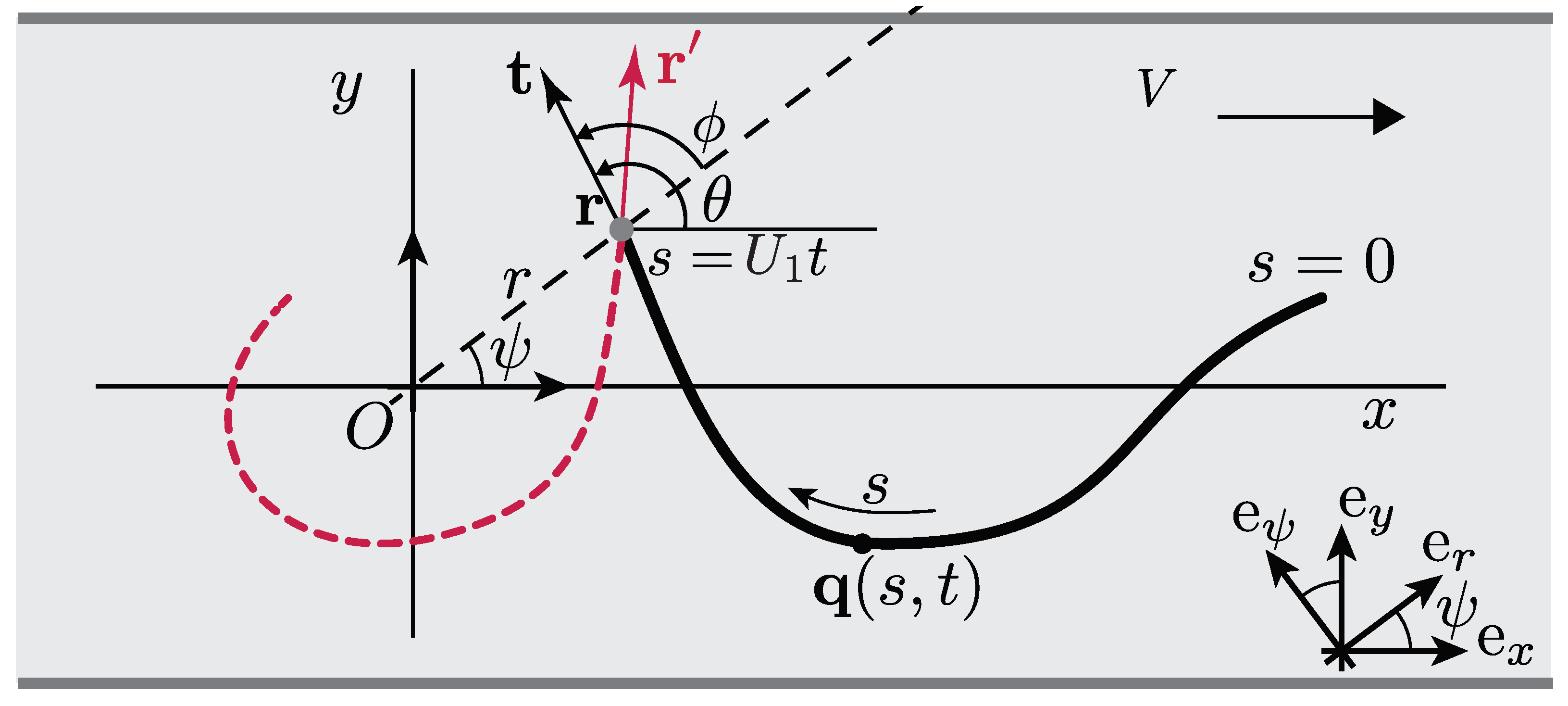
Now let $\left\{r\right(s),\psi (s\left)\right\}$ be the polar coordinates of the contact point $\mathit{r}\left(s\right)$, and let $\theta \left(s\right)$ be the angle between ${\mathit{e}}_x$ and $\mathit{t}$. Referring to Figure 11, we resolve $\mathit{t}$, ${\mathit{r}}^{\prime }$, and ${\mathit{e}}_x$ into the polar basis $({\mathit{e}}_r,{\mathit{e}}_{\psi })$. The two components of (17) then take the form

$$r^{\prime }=cos(\theta -\psi )+\frac{V}{U_1}cos\psi ,$$

(18)

$$r{\psi }^{\prime }=sin(\theta -\psi )-\frac{V}{U_1}sin\psi .$$

(19)

We need one more equation to close the system. To find it, we note that the DVT model predicts that the curvature ${\theta }^{\prime }$ of the trace at the contact point depends only on r and $\theta -\psi$ to a good approximation:

$${\theta }^{\prime }=\kappa (r,\theta -\psi ).$$

(20)

The function $\kappa$ is determined by fitting to the predictions of the DVT model [23].

Equation (7) are three coupled nonlinear autonomous first-order differential equations for $r\left(s\right)$, $\psi \left(s\right)$ and $\theta \left(s\right)$. They involve only a single parameter, the dimensionless belt speed $V/U_1$. The equations remain unchanged when r and s are nondimensionalized by, e.g., the radius $R_c$ of steady coiling on a motionless surface. We call Equation (7) the ‘geometric model’ (GM). The GM equations were solved using the NDSolve function of Mathematica [25]. The parameter $V/U_1$ was varied quasi-statically during the simulations, over a time scale large compared with the dominant period of the patterns. Additional solutions were obtained using the continuation and bifurcation analysis software package AUTO-07p [26] to determine the type of each bifurcation encountered as $V/U_1$ was varied. The convergence of the solutions was verified by showing that they remained essentially identical when the tolerance parameters were increased by an order of magnitude.

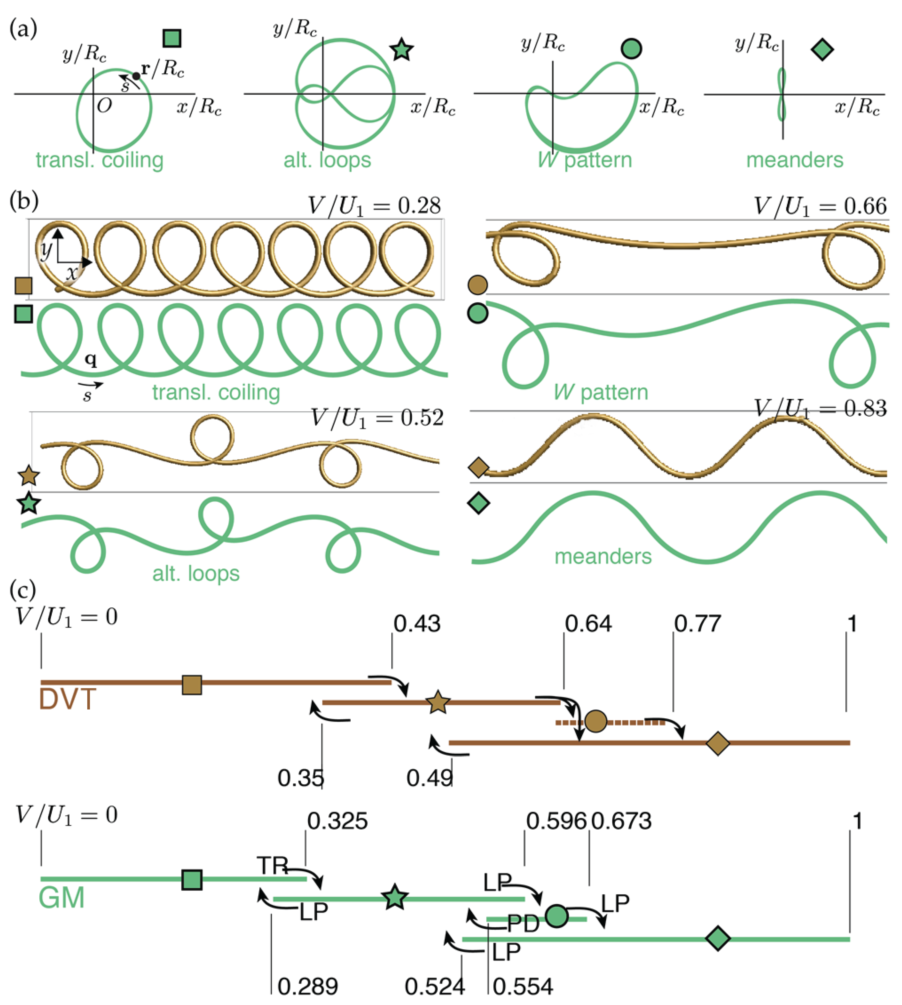
Figure 12 presents a detailed comparison of the GM (green) and DVT (brown) predictions. Part (a) shows the orbits $\mathit{r}\left(s\right)$ for the four periodic patterns in the frame of the nozzle as predicted by the GM. Part (b) shows the corresponding patterns $\mathit{q}(s,t)$ predicted by both DVT and the GM for four different values of $V/U_1=0.28$ (meanders), 0.52 (alternating loops), 0.66 (W pattern) and 0.83 (meanders). The GM captures all the patterns originally predicted by the DVT simulations, in the proper order as $V/U_1$ varies. The horizontal lines in part (c) show the stability ranges of the patterns. In the original DVT simulations, bifurcations between the patterns were found to be hysteretic: the value of $V/U_1$ at which each transition occurs depends on whether $V/U_1$ is increasing or decreasing. This feature of the solutions is reproduced by the GM, which in addition allows one to characterize the type of bifurcation involved in each case. The bifurcations are fold points, except for two: a torus bifurcation from translated coiling to alternating loops as $V/U_1$ increases, and a period-doubling bifurcation from the W pattern to alternating loops as $V/U_1$ decreases. Finally, the GM explains why the W pattern was observed in DVT simulations with an increasing belt velocity, but not with a decreasing one.

8. Discussion

A striking feature of many of the FMSM patterns is their fore–aft symmetry with respect to the direction of motion of the belt. Experimentally observed patterns having this symmetry include meanders, alternating loops, two-by-two, translated coiling, and the W pattern. Moreover, kinematic reconstructions reveal that other patterns belong to this group, including double coiling, double meanders, and stretched coiling. Viewing such patterns from above provides no indication of which way the belt is moving. The situation for patterns lacking fore–aft symmetry is quite different: once any of these patterns have been associated with a direction of belt motion by means of one observation, subsequent observations will always be able to indicate which way the belt is moving.

Figure 3 and Table 1 shows that several patterns lack fore–aft symmetry: bunched meanders, braiding, bunched double coiling, slanted loops, double meanders, and sidekicks. Different factors seem to be responsible for this. First, in some of these patterns (braiding, bunched double coiling, slanted loops), the free part of the falling thread makes contact with an ‘earlier’ portion of the thread that was previously laid down on the belt. Such self-interaction does not occur in the DVT simulations, where the fluid laid down on the belt is continuously ‘whisked away’ to make the boundary condition clean. In laboratory experiments, however, self-interaction in the case of certain patterns cannot be avoided, and breaks the fore–aft symmetry. A second symmetry-breaking factor is a large amplitude of the pattern relative to its wavelength. An example is bunched meanders, which weakly break the fore–aft symmetry of their smaller-amplitude counterparts (i.e., normal meanders). A third potential symmetry-breaking factor may be the presence of two dominant frequencies, as in double meanders.

However, a closer look shows that fore–aft symmetry is always imperfect even for patterns that look symmetric to the naked eye. This is clear from the DVT spectra of the longitudinal motion (red lines) shown in the right-hand colum of Figure 10. These all have noticeable power at zero frequency, indicating a constant offset of the contact point trajectory in the x-direction relative to the center of the nozzle. This offset is visible in the contact point trajectories shown at upper right in each panel of the left-hand column of Figure 10. Physically, the offset reflects the fact that the gravitational heel structure of the thread near the belt (Figure 7) does not itself have fore–aft symmetry, because the thread is dragged in only one direction by the belt. In this context it is worth noting that kinematic reconstructions of the DVT contact point trajectories that neglect the power at zero frequency do exhibit fore–aft symmetry (left-hand column of Figure 10, lower-right portion of each panel).

While existing studies provide significant physical insight, much remains to be done before we fully understand the FMSM. On the experimental side, observations obtained using much higher values of the dimensionless parameter ${\Pi }_1={({\nu }^5/g{Q}^3)}^{1/5}$ would be desirable. The reason is that the multivaluedness of the steady coiling frequency $\Omega \left(H\right)$ increases with ${\Pi }_1$ [10]. Values of ${\Pi }_1\approx {10}^5$ are easy to achieve in the laboratory using high-viscosity silicone oil and very low flow rates [11]. A greater degree of multivaluedness indicates a greater number of possible nonlinear interactions among the inertio-gravitational pendulum modes. Such interactions should lead to an even richer phase diagram of FMSM patterns than the one we have studied here. From the theoretical point of view, the FMSM can be regarded as a weakly forced nonlinear oscillator. An ambitious but worthy goal would be to develop an asymptotic nonlinear oscillator theory for the FMSM patterns by considering the mode interactions mentioned above.

References

- Chiu-Webster, S.; Lister, J.R. The fall of a viscous thread onto a moving surface: A ‘fluid mechanical sewing machine’. J. Fluid Mech. 2006, 569, 89–111. [Google Scholar] [CrossRef]
- Barnes, G.; Woodcock, R. Liquid rope-coil effect. Am. J. Phys. 1958, 26, 205–209. [Google Scholar] [CrossRef]
- Barnes, G.; MacKenzie, R. Height of fall versus frequency in liquid rope-coil effect. Am. J. Phys. 1959, 27, 112–115. [Google Scholar] [CrossRef]
- Cruickshank, J.O. Viscous Fluid Buckling: A Theoretical and Experimental Analysis with Extensions to General Fluid Stability. Ph.D. Thesis, Iowa State University, Ames, IA, USA, 1980. [Google Scholar]
- Cruickshank, J.O.; Munson, B.R. Viscous fluid buckling of plane and axisymmetric jets. J. Fluid Mech. 1981, 113, 221–239. [Google Scholar] [CrossRef]
- Huppert, H.E. The intrusion of fluid mechanics into geology. J. Fluid Mech. 1986, 173, 557–594. [Google Scholar] [CrossRef] [Green Version]
- Griffiths, R.W.; Turner, J.S. Folding of viscous plumes impinging on a density or viscosity interface. Geophys. J. 1988, 95, 397–419. [Google Scholar] [CrossRef]
- Mahadevan, L.; Ryu, W.S.; Samuel, A.D.T. Fluid ‘rope trick’ investigated. Nature 1998, 392, 140, Erratum in Nature 2000, 403, 502. [Google Scholar] [CrossRef]
- Maleki, M.; Habibi, M.; Golestanian, R.; Ribe, N.M.; Bonn, D. Liquid rope coiling on a solid surface. Phys. Rev. Lett. 2004, 93, 214502. [Google Scholar] [CrossRef]
- Ribe, N.M.; Huppert, H.E.; Hallworth, M.A.; Habibi, M.; Bonn, D. Multiple coexisting states of liquid rope coiling. J. Fluid Mech. 2006, 555, 275–297. [Google Scholar] [CrossRef] [Green Version]
- Ribe, N.M.; Habibi, M.; Bonn, D. Stability of liquid rope coiling. Phys. Fluids 2006, 18, 084102. [Google Scholar] [CrossRef] [Green Version]
- Habibi, M.; Maleki, M.; Golestanian, R.; Ribe, N.M.; Bonn, D. Dynamics of liquid rope coiling. Phys. Rev. E 2006, 74, 066306. [Google Scholar] [CrossRef] [PubMed]
- Habibi, M.; Rahmani, Y.; Bonn, D.; Ribe, N.M. Buckling of liquid columns. Phys. Rev. Lett. 2010, 104, 074301. [Google Scholar] [CrossRef] [PubMed] [Green Version]
- Habibi, M.; Hosseini, S.H.; Khatami, M.H.; Ribe, N.M. Liquid supercoiling. Phys. Fluids 2014, 26, 024101. [Google Scholar] [CrossRef]
- Cruickshank, J.O. Low-Reynolds-number instabilities in stagnating jet flows. J. Fluid Mech. 1988, 193, 111–127. [Google Scholar] [CrossRef]
- Tchavdarov, B.; Yarin, A.L.; Radev, S. Buckling of thin liquid jets. J. Fluid Mech. 1993, 253, 593–615. [Google Scholar] [CrossRef]
- Blount, M.J. Bending and Buckling of a Falling Viscous Thread. Ph.D. Thesis, University of Cambridge, Cambridge, UK, 2010. [Google Scholar]
- Ribe, N.M. Coiling of viscous jets. Proc. R. Soc. London Ser. A Math. Phys. Eng. Sci. 2004, 460, 3223–3239. [Google Scholar] [CrossRef]
- Ribe, N.M.; Lister, J.R.; Chiu-Webster, S. Stability of a dragged viscous thread: Onset of ‘stitching’ in a fluid mechanical ‘sewing machine’. Phys. Fluids 2006, 18, 124105. [Google Scholar] [CrossRef]
- Morris, S.; Dawes, J.H.P.; Ribe, N.M.; Lister, J.R. Meandering instability of a viscous thread. Phys. Rev. E 2008, 77, 066218. [Google Scholar] [CrossRef] [Green Version]
- Blount, M.J.; Lister, J.R. The asymptotic structure of a slender dragged viscous thread. J. Fluid Mech. 2011, 674, 489–521. [Google Scholar] [CrossRef]
- Brun, P.T.; Ribe, N.M.; Audoly, B. A numerical investigation of the fluid mechanical sewing machine. Phys. Fluids 2012, 24, 043102. [Google Scholar] [CrossRef] [Green Version]
- Brun, P.T.; Audoly, B.; Ribe, N.M.; Eaves, T.S.; Lister, J.R. Liquid ropes: A geometrical model for thin viscous jet instabilities. Phys. Rev. Lett. 2015, 114, 174501. [Google Scholar] [CrossRef] [PubMed] [Green Version]
- Audoly, B.; Clauvelin, N.; Brun, P.T.; Bergou, M.; Grinspun, E.; Wardetzky, M. A discrete geometric approach for simulating the dynamics of thin viscous threads. J. Comp. Phys. 2013, 253, 18–49. [Google Scholar] [CrossRef] [Green Version]
- Wolfram Research, Inc. Mathematica, Version 13.0.0; Wolfram Research, Inc.: Champaign, IL, USA, 2021; Available online: https://www.wolfram.com/mathematica (accessed on 1 February 2022).
- Doedel, E.J.; Oldeman, B.E. AUTO-07P: Continuation and Bifurcation Software for Ordinary Differential Equations; Technical Report; Concordia University: Montréal, QC, Canada, 2007. [Google Scholar]
Figure 1.
Behaviors of a viscous thread falling onto a motionless surface. (a) Steady coiling for cS, mL·s, and cm. The definitions of the coil radius R and the radius of the thread at the contact point are shown. The structure comprises a long and nearly vertical tail, the coil, and a pile of fluid previously laid down by the coiling. (b) Axisymmetric stagnation flow for cS, mL·s, and cm. (c) Coiling with an unstable pile for cS, mL·s, and cm.
Figure 2.
A laboratory apparatus for studying the FMSM. The units on the ruler are centimeters (left) and inches (right). Photograph courtesy of J. R. Lister.
Figure 3.
Stitch patterns observed in the FMSM. Photographs courtesy of J.R. Lister.
Figure 4.
Stitch patterns of the FMSM as a function of fall height H and belt speed V, for silicone oil with S and cm·s. Upright and inverted triangles indicate observations made while increasing and decreasing the belt speed, respectively. Grey shaded regions indicate ranges of H for which the frequency of liquid thread coiling, calculated for the parameters of the experiment using the method of Ribe [18], is multivalued. Figure adapted from Figure 3 of [20].
Figure 5.
Coiling frequency as a function of the fall height H for g·cm, cS, dyne·cm, cm and mL·s. The red curve was calculated numerically using the method of Ribe [18]. Portions of the curve corresponding to the different steady coiling regimes are indicated: V (viscous), G (gravitational), IG (inertiogravitational), and I (inertial). Dotted portions of the curve represent coiling that is unstable to small perturbations. Dashed lines with slope are the first three pendulum frequencies of the tail of the thread, with the order of each mode indicated by the number to the left.
Figure 6.
Onset of meandering for golden syrup ( g·cm, S), cm s, and cm. (a) Critical belt speed as a function of fall height. Circles: experimental measurements. Solid line: prediction of the linear stability analysis described in the text. Dotted line (nearly indistinguishable from the solid line): axial velocity at the bottom of a thread coiling on a motionless surface for the same experimental parameters. (b) Angular frequency of oscillation as a function of fall height. Circles: experimental measurements. Solid line: prediction of the linear stability analysis. Dotted line: angular frequency of steady liquid thread coiling on a motionless surface for the same experimental parameters. Figure adapted from Figures 5 and 7 of [19].
Figure 7.
‘Gravitational heel’ shape of a dragged viscous thread at the onset of meandering, for the parameters of the experiment of Figure 6. The shape was calculated numerically using the method of Ribe et al. [19]. The horizontal scale is exaggerated by a factor of 15 relative to the vertical scale. Figure adapted from Figure 6 of [19].
Figure 8.
Phase diagram for the patterns at low fall heights . Numerically predicted and experimentally observed patterns as functions of and are indicated by vertical lines and circles, respectively. The patterns corresponding to each color are shown as insets. White spaces between vertical bars of different colors indicate ranges of belt speeds for which the automatic pattern recognition gave ambiguous results. Figure adapted from Figure 6 of [22].
Figure 9.
Main portion: phase diagram of the FMSM constructed using DVT for , , and no surface tension (). The patterns shown as insets include translated coiling (A, red), meanders (B, blue), alternating loops (C, green), disordered patterns (D, grey), double coiling (E, pink), double meanders (F, purple), and stretched coiling (H, yellow). The dimensionless frequency of liquid thread coiling is shown beneath the phase diagram, with multivalued intervals highlighted. Inset: phase diagram determined experimentally [20] with , and (top). Additional patterns include the W pattern (yellow circled in black) and slanted loops (blue circled in black). The corresponding coiling frequency is also shown (bottom). Figure adapted from Figure 7 of [22].
Figure 10.
Spectral characteristics of three FMSM patterns: translated coiling (A), alternating loops (B), and double coiling (C). See the main text for a detailed discussion. Figure adapted from Figure 10 of [22].
Figure 11.
Geometry of a falling viscous thread in the vicinity of its contact point with a moving belt. Figure adapted from Figure 3 of [23].
Figure 12.
Comparison of the predictions of the GM (green) and full DVT simulations (brown). See the main text for a detailed discussion. Figure adapted from Figure 5 of [23].