
Subordination Involving Regular Coulomb Wave Functions


Department of Mathematics and Statistics, College of Science, King Faisal University, Al Hasa 31982, Saudi Arabia
Symmetry 2022, 14(5), 1007; https://0-doi-org.brum.beds.ac.uk/10.3390/sym14051007
Submission received: 8 April 2022
/
Revised: 30 April 2022
/
Accepted: 10 May 2022
/
Published: 16 May 2022
(This article belongs to the Special Issue Complex Analysis, in Particular Analytic and Univalent Functions)
Abstract
:The functions , , , map the unit disc to a domain which is symmetric about the x-axis. The Regular Coulomb wave function (RCWF) is a function involving two parameters L and , and is symmetric about these. In this article, we derive conditions on the parameter L and for which the normalized form of are subordinated by . We also consider the subordination by and , . A few more subordination properties involving RCWF are discussed, which leads to the star-likeness of normalized Regular Coulomb wave functions.
1. Introduction
The Regular Coulomb wave function (RCWF) defined in the complex plane is an entire function and closely associated with the well-known classical Bessel function. The Coulomb wave functions have a rich literature (See [1,2,3,4,5,6,7,8,9,10] and references therein) in terms of mathematical and numerical research articles and its applications in various branches of physics, especially in nuclear physics. The symmetrical property of RCWF is established in [11]. Entire functions have good geometric characterizations in the unit disc. In this sense, the exploration of the geometric nature of Coulomb wave functions is limited [4,12]. The aim of this article is to contribute some results on the geometric properties of RCWF.
The Coulomb differential equation [13] is a second-order differential equation of the form
that asserts two independent solutions, namely regular and irregular Coulomb wave functions. In terms of Kummer confluent hypergeometric functions , the RCWF is defined as
In this case, and
For the study of the geometric characterization of RCWF, we need a normalized form such as as or . Clearly, defined in (2) does not process such a normalization. Hence, we consider the following two normalizations:
By a calculation, it can be shown from (1) that satisfies the differential equation
while the function is the solution of the differential equation
Let denote the class of normalized analytic functions f in the open unit disk satisfying . Denote by and , respectively, the widely studied subclasses of consisting of univalent (one-to-one) star-like and convex functions. Geometrically, if the linear segment , lies completely in whenever , while if is a convex domain. Related to these subclasses is the Cárathèodory class consisting of analytic functions p satisfying and in . Analytically, if , while if .
For two analytic functions f and g in , the function f is subordinate to g, written as or , if there is an analytic self-map of satisfying and , .
Consider now the class of analytic functions in satisfying where is an analytic function with a positive real impact on , and . This article considers three different , namely , and .
For and , denote the class as . This family has been widely studied by several authors and most notably by Janowski in [14], and the class is also referred to as Janowski class of functions. The class contains several known classes of functions for judicious choices of A and B. For instance, if , then is the class of functions satisfying in . In the limiting case , the class reduces to the classical Cárathèodory class .
The class of Janowski star-like functions consists of satisfying
while the Janowski convex functions are functions satisfying
For , is the classical class of star-like functions of order ; , and . These are all classes that have been widely studied; see, for example, the works of [14,15,16].
The next important class is related to the right half of lemniscate of Bernoulli given by The functions in satisfying are known as lemniscate Cárathèodory function, and the corresponding class is denoted by . A lemniscate Cárathèodory function is also Cárathèodory function and hence univalent. The lemniscate star-like class consists of functions such that . The class is known as a class of lemniscate convex functions.
The third important class that is considered in sequence relates with the exponential functions . The functions in satisfying is known as the exponential Cárathèodory function, and the corresponding class is denoted by . The exponential star-like class consists of functions such that . The class is known as a class of exponential convex functions.
The inclusion properties of special functions in the geometric classes are well known [4,12,17,18,19,20,21,22]. However, there are limited articles regarding the inclusion of RCWF in the classes of geometric functions theory. It is proved in [4] that for , the function is leminiscate star like provided that
It is also shown that is exponentially star like provided that
The radius of star-likeness, univalency, is discussed in [12] by using the Weierstrassian canonical product expansion of RCWF. It is proved that for and , the radius of star-likeness of the order for the functions is the smallest positive root of
The star-likeness of is discussed in ([12], Theorem 4). The conditions for which were also found in same results ([12], Theorem 4). However, it seems that the obtained condition for which is not correct with that fact that , while as per the requirement of ([12], Lemma 2), it should be .
The aim of this study is to contribute more results related to the inclusion of normalized RCWF in the classes of univalent functions theory. In Section 2, we state a proof of the results in which the function is subordinated by three functions, , and . We explain our results through a graphical representation in some special cases. The star-likeness for in the shifted disc is also considered.
Throughout this study, we used the principle of differential subordination [23,24], which is an important tool in the investigation of various classes of analytic functions to proof main result.
Lemma 1
Lemma 2
Lemma 3
The following Lemma holds for r and s as stated in Lemma 2.
Lemma 4.
Consider s and r as in (7) with . For any , the following inequalities are true:
Proof.
For the r and s along with , we have
A calculation shows
For a fixed , has a zero only at in , and further for ,
This implies that g has a local minimum at and hence
This complete the proof. □
2. Geometric Properties of Coulomb Wave Functions (CWF)
2.1. Subordination by
In [4], sufficient conditions based on L and is derived for which , that is , is Lemniscate star like. This section derives conditions on L and for which , which we termed as is the Lemniscate Catathéodory function.
Theorem 1.
For , suppose that
then .
Proof.
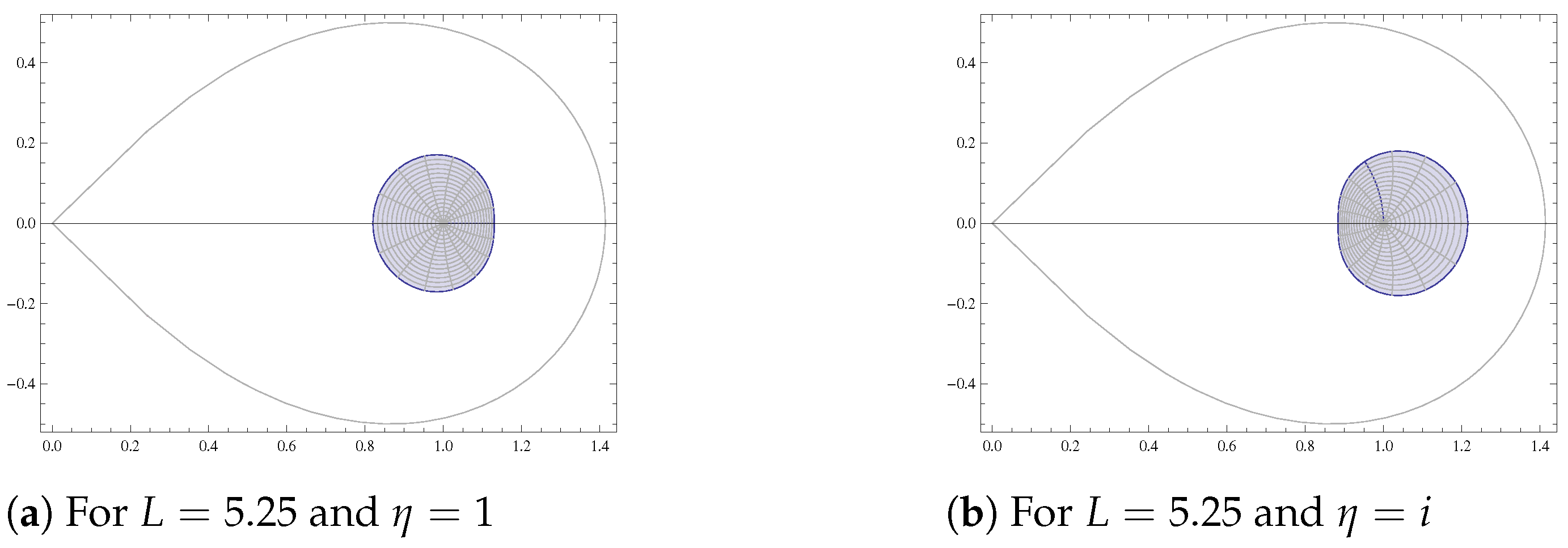
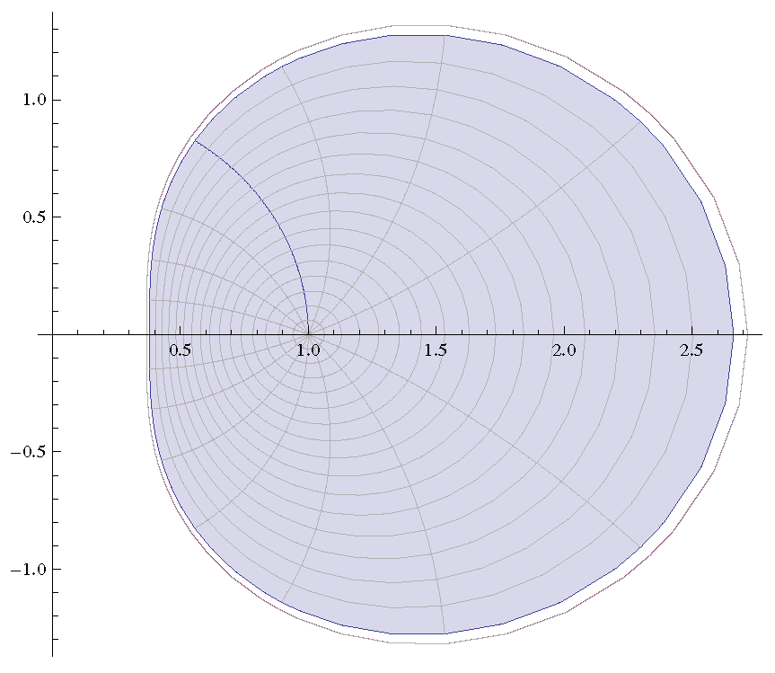
It is well known that for univalent function g, if , then . Using this fact, we chose some real and complex , and validated Theorem 1. For the first case, consider , and L is a real number. Using Theorem 1, in both cases, . This fact is represented in Figure 1.
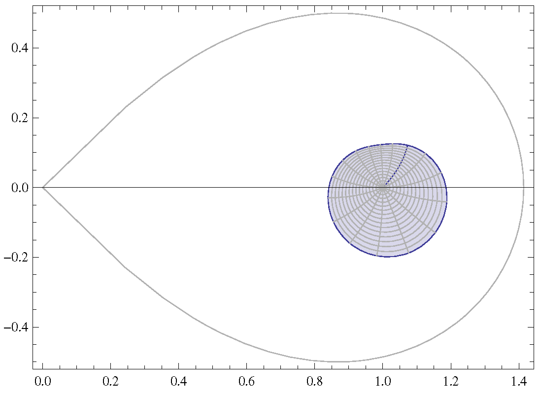
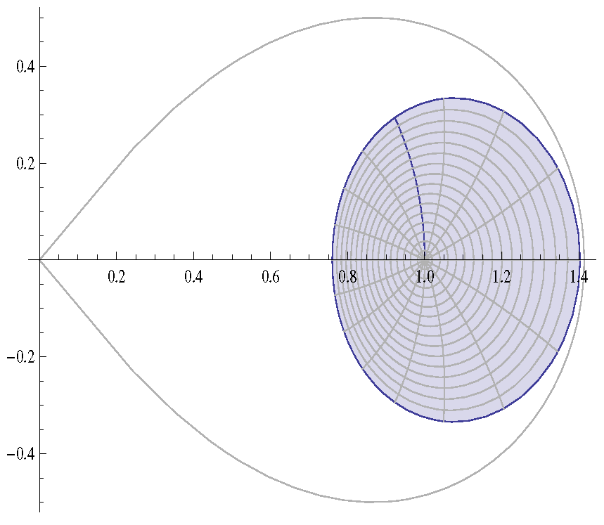
We consider another case by taking . By Theorem 1, in this case for real , and Figure 2 validate the result.
2.2. Subordination by
In this part we proved that result related to the subordination and which describe the nature of and in the disc center at and radius A. The results in this section are proved by using Lemma 2.
Theorem 2.
For and , suppose that
Then, .
Proof.
Let and define as
It is clear from (14) that . We shall apply Lemma 2 to show that , which further implies .
Now, for , let
It follows by elementary trigonometric identities that
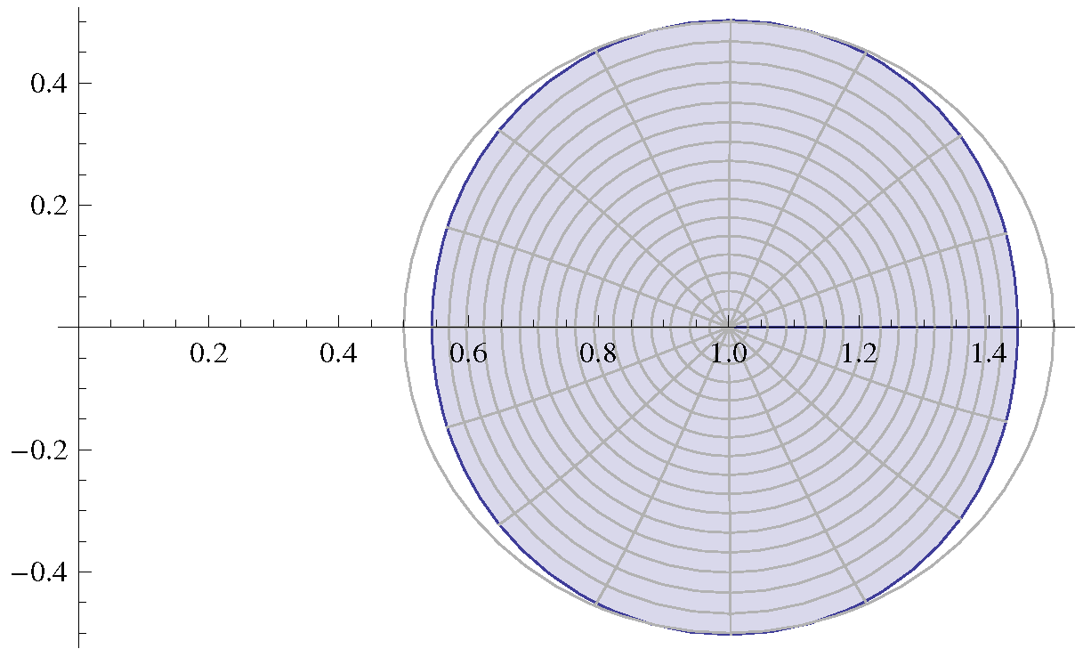
Again to validate the Theorem 2, we fix and . Lets L be real and then as per Theorem 2, . The Figure 3 indicates that the lower bound for L is possible sharp.
Our next result is about the starlikenes of in the disc .
Theorem 3.
For and , suppose that
Then, .
Proof.
To prove the result consider
A calculation yield
From (6) it follows that
Let and define as
It is clear from (18) that . We shall apply Lemma 2 and proceed similar to the proof of Theorem 2 to show that . Substitute r and s into (18), and a simplification leads to
provided .
In view of Lemma 2, it concludes that , which is equivalent to
for some analytic functions such that . A simplification gives
This concludes the result. □
2.3. Subordination by
In this part, we derive sufficient conditions on L and for which . The exponential starlikeness of is discussed in [4]. It is worthy to note here that exponential starlikeness is equivalent to .
Theorem 4.
For , suppose that
Then .
Proof.
2.4. Subordination by
Theorem 5.
Let and . Suppose that
Then,
provided .
Proof.
Clearly, by the given hypothesis, , and hence . This implies that . From Lemma 1 it follows
This completes the proof. □
Define the function
A series of calculation and simplification leads to
From (6), it follows that
Let and define
Denoting and , we have
By choosing in Theorem 5, we have the following result on the star-likeness of .
Corollary 1.
For , suppose that . Then, is star like provided that for .
Remark 1.
The condition for the star-likeness of is provided in ([12], Theorem 4) which is the same as stated in Corollary 1.
3. Conclusions
This study finds the conditions for the parameters L and for which the normalized function is subordinated by three different functions , , and .
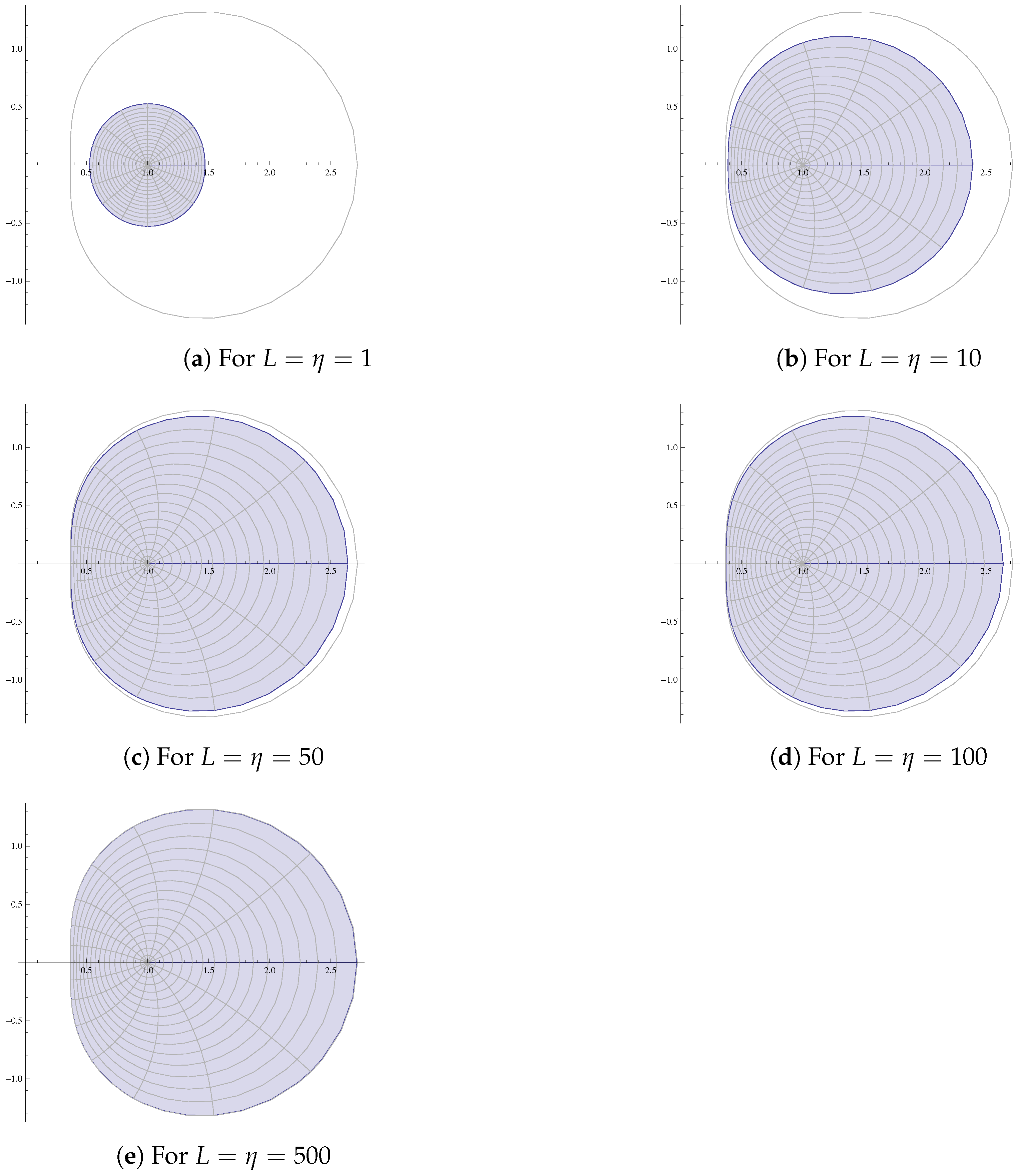
We already interpreted Theorems 1, 2 and 4 graphically. Figure 3 describes the sharpness of Theorem 2. On the other hand, Figure 4 indicates the situation related to Theorem 4. However, we were unable to obtain examples with a similar sharpness using Theorem 1. Thus, it is expected show some improvement in the obtained results. For example, let , and then by Theorem 4, for . However, Figure 5 indicates that if L is real, then it can be lower than 1 for .
Similarly, for , Theorem 1 implies that for
However, for real L, it follows from Figure 6 that L can be down to .
From the above discussion, we can finally conclude that Theorems 1, 2 and 4 are completely valid with respect to the stated hypothesis. However, for some special choice of parameter , there is a possibility for improvement.
This article also derives the conditions for the star-likeness of in the disc and . With the special case for and , the results lead to a known result ([12], Theorem 4).
Funding
This work was supported through the Annual Funding track by the Deanship of Scientific Research, Vice Presidency for Graduate Studies and Scientific Research, King Faisal University, Saudi Arabia [Project No. AN00097].
Institutional Review Board Statement
Not Applicable.
Informed Consent Statement
Not Applicable.
Data Availability Statement
Not Applicable.
Conflicts of Interest
The authors declare no conflict of interest.
References
- Baricz, Á. Turán type inequalities for regular Coulomb wave functions. J. Math. Anal. Appl. 2015, 430, 166–180. [Google Scholar] [CrossRef]
- Ikebe, Y. The zeros of regular Coulomb wave functions and of their derivatives. Math. Comput. 1975, 29, 878–887. [Google Scholar]
- Miyazaki, Y.; Kikuchi, Y.; Cai, D.; Ikebe, Y. Error analysis for the computation of zeros of regular Coulomb wave function and its first derivative. Math. Comput. 2001, 70, 1195–1204. [Google Scholar] [CrossRef] [Green Version]
- Aktaş, İ. Lemniscate and exponential starlikeness of regular Coulomb wave functions. Stud. Sci. Math. Hung. 2020, 57, 372–384. [Google Scholar] [CrossRef]
- Humblet, J. Bessel function expansions of Coulomb wave functions. J. Math. Phys. 1985, 26, 656–659. [Google Scholar] [CrossRef] [Green Version]
- Humblet, J. Analytical structure and properties of Coulomb wave functions for real and complex energies. Ann. Phys. 1984, 155, 461–493. [Google Scholar] [CrossRef]
- Thompson, I.J.; Barnett, A.R. Coulomb and Bessel functions of complex arguments and order. J. Comput. Phys. 1986, 64, 490–509. [Google Scholar] [CrossRef]
- Michel, N. Precise Coulomb wave functions for a wide range of complex l, η and z. Comput. Phys. Commun. 2007, 176, 232–249. [Google Scholar] [CrossRef] [Green Version]
- Štampach, F.; Šťovíček, P. Orthogonal polynomials associated with Coulomb wave functions. J. Math. Anal. Appl. 2014, 419, 231–254. [Google Scholar] [CrossRef]
- Nishiyama, T. Application of Coulomb wave functions to an orthogonal series associated with steady axisymmetric Euler flows. J. Approx. Theory 2008, 151, 42–59. [Google Scholar] [CrossRef] [Green Version]
- Gaspard, D. Connection formulas between Coulomb wave functions. J. Math. Phys. 2018, 59, 112104. [Google Scholar] [CrossRef]
- Baricz, Á.; Çaǧlar, M.; Deniz, E.; Toklu, E. Radii of starlikeness and convexity of regular Coulomb wave functions. arXiv 2016, arXiv:1605.06763. [Google Scholar]
- Abramowitz, M.; Stegun, I.A. Handbook of Mathematical Functions, with Formulas, Graphs, and Mathematical Tables; Dover Publications, Inc.: New York, NY, USA, 1966. [Google Scholar]
- Janowski, W. Some extremal problems for certain families of analytic functions. I. Ann. Polon. Math. 1973, 28, 297–326. [Google Scholar] [CrossRef] [Green Version]
- Ali, R.M.; Ravichandran, V.; Seenivasagan, N. Sufficient conditions for Janowski starlikeness. Int. J. Math. Math. Sci. 2007, 2007, 062925. [Google Scholar] [CrossRef] [Green Version]
- Ali, R.M.; Chandrashekar, R.; Ravichandran, V. Janowski starlikeness for a class of analytic functions. Appl. Math. Lett. 2011, 24, 501–505. [Google Scholar] [CrossRef] [Green Version]
- Kanas, S.; Mondal, S.R.; Mohammed, A.D. Relations between the generalized Bessel functions and the Janowski class. Math. Inequal. Appl. 2018, 21, 165–178. [Google Scholar]
- Mondal, S.R.; Swaminathan, A. Geometric properties of generalized Bessel functions. Bull. Malays. Math. Sci. Soc. 2012, 35, 179–194. [Google Scholar]
- Madaan, V.; Kumar, A.; Ravichandran, V. Lemniscate convexity of generalized Bessel functions. Stud. Sci. Math. Hung. 2019, 56, 404–419. [Google Scholar] [CrossRef]
- Naz, A.; Nagpal, S.; Ravichandran, V. Exponential starlikeness and convexity of confluent hypergeometric, Lommel, and Struve functions. Mediterr. J. Math. 2020, 17, 22. [Google Scholar] [CrossRef]
- Naz, A.; Nagpal, S.; Ravichandran, V. Star-likeness associated with the exponential function. Turk. J. Math. 2019, 43, 1353–1371. [Google Scholar] [CrossRef]
- Baricz, Á.; Štampach, F. The Hurwitz-type theorem for the regular Coulomb wave function via Hankel determinants. Linear Algebra Appl. 2018, 548, 259–272. [Google Scholar] [CrossRef] [Green Version]
- Miller, S.S.; Mocanu, P.T. Differential subordinations and inequalities in the complex plane. J. Differ. Equ. 1987, 67, 199–211. [Google Scholar] [CrossRef] [Green Version]
- Miller, S.S.; Mocanu, P.T. Differential Subordinations. In Monographs and Textbooks in Pure and Applied Mathematics; Dekker: New York, NY, USA, 2000; p. 225. [Google Scholar]
- Madaan, V.; Kumar, A.; Ravichandran, V. Starlikeness associated with lemniscate of Bernoulli. Filomat 2019, 33, 1937–1955. [Google Scholar] [CrossRef] [Green Version]
Figure 1.
Image of for .

Figure 2.
Image of for .

Figure 3.
Image of for and .

Figure 4.
Cases for for .

Figure 5.
Image of for and .

Figure 6.
Image of for and .

Publisher’s Note: MDPI stays neutral with regard to jurisdictional claims in published maps and institutional affiliations. |
© 2022 by the author. Licensee MDPI, Basel, Switzerland. This article is an open access article distributed under the terms and conditions of the Creative Commons Attribution (CC BY) license (https://creativecommons.org/licenses/by/4.0/).
Share and Cite
MDPI and ACS Style
Mondal, S.R. Subordination Involving Regular Coulomb Wave Functions. Symmetry 2022, 14, 1007. https://0-doi-org.brum.beds.ac.uk/10.3390/sym14051007
AMA Style
Mondal SR. Subordination Involving Regular Coulomb Wave Functions. Symmetry. 2022; 14(5):1007. https://0-doi-org.brum.beds.ac.uk/10.3390/sym14051007
Chicago/Turabian StyleMondal, Saiful R. 2022. "Subordination Involving Regular Coulomb Wave Functions" Symmetry 14, no. 5: 1007. https://0-doi-org.brum.beds.ac.uk/10.3390/sym14051007
Note that from the first issue of 2016, this journal uses article numbers instead of page numbers. See further details here.