A New Uncertain Interest Rate Model with Application to Hibor

Abstract

This paper proposes a new interest rate model by using uncertain mean-reverting differential equation. Based on the model, the pricing formulas of the zero-coupon bond, the interest rate ceiling and interest rate floor are derived respectively according to Yao-Chen formula. The symmetry appears in mathematical formulations of the interest rate ceiling and interest rate floor pricing formula. Furthermore, the model is applied to depict Hong Kong interbank offered rate (Hibor). Finally the parameter estimation by the method of moments and hypothesis test is completed.

1. Introduction

The interest rate plays a vital role in the economy and financial products in policy making. The interest rate is a powerful control tool for managing the market. Firstly, it is necessary to price and hedge fixed-income derivatives. Secondly, it reflects market participant expectations about interest rates changes and their assessment of the monetary policy conditions. Considering the significance of interest rate, some economists and financial institutions modeled the term structure of interest rates as the research object. In 1973, the first interest rate model was established by Merton [1], based on the model developed by Ho and Lee [2]. Vasicek [3] proposed an equilibrium model in 1977. Cox et al. [4] developed the Cox-Ingersoll-Ross model in 1985 to ensure the interest rate could remain positive all the time. In above quantitative models, the risky part of the interest rate models is always driven by Brownian motion with independent and stationary increment.

As we all know, an enormous amount of historical data is needed to build models when using probability theory. However, the sample number is often not enough for us to build a probability distribution in many cases. For dealing with the problem, Liu [5] established uncertainty theory to model belief degree as a branch of axiomatic mathematics in 2007. To describe dynamic uncertain systems quantitatively, Liu [6] defined uncertain process and constructed uncertain differential equation in 2008. Due to its high influence, uncertain differential equation had been investigated a lot.

Under the linear growth condition and Lipschitz continuous condition, Chen and Liu [7] presented methods to solve linear uncertain differential equations in 2010. Following that, Gao [8] generalized the conditions of the coefficients. Yao-chen formula, a connection between uncertain differential equations and ordinary differential equations through $\alpha$-path, was proved by Yao and Chen [9].

In order to estimate unknown parameters in uncertain differential equation with the observed data, Yao and Liu [10] firstly provided the method of moments. Following that, generalized moment estimation was investigated by Liu [11] and the relationship between them were proposed. Least squares estimation was solved by Sheng [12] through minimum noise. Furthermore, maximum likelihood estimation [13] and minimum cover estimation [14] were investigated. In addition, uncertain hypothesis test was firstly founded by Ye [15] to judge whether the hypothesis is correct or not rationally.

Uncertain differential equation was derived in uncertain stock model in finance by Liu [16] in 2009 firstly, then European call option and European put option price formulas were obtained. Following that, Chen [17] presented the American option pricing formulas. Then more different kinds of exotic options were explored. Meanwhile, the construction of uncertain stock models became another hot spot. Considering the stock price swing around some medium price in long-run, Peng and Yao [18] investigated the uncertain mean-reverting model. Chen et al. [19] discussed an uncertain stock model with periodic dividends according to cannoical process. Considering the phenomenon of sudden drift in real financial market, Yu [20] developed the uncertain stock model with jumps. To deal with the nonliear more reversion phenomenon, Dai et al. [21] formulated the uncertain exponential Ornstein-Uhlenbeck model.

The Ho and Lee model [2], Vasicek model [3] and Cox-Ingersoll-Ross (CIR) model [4] were three classic interest rate model based on stochastic differential equation. Chen and Gao [22] derived three different uncertain term structure models in 2013 as the counterparts of among stochastic models, then they discussed the zero-coupon bond price problem. Following that, Zhang et al. [23] discussed the valution of interest rate ceiling and floor in uncertain Vasicek model. Jiao and Yao [24] discussed the zero-coupon bond price problem with uncertain CIR model in 2015. Furthermore, Sun et al. [25] proposed a new interest rate model derived by exponential Ornstein-Uhlenbeck equation and then obtained the pricing formulas of the zero-coupon bond, interest rate ceiling and interest rate floor. In addition, Zhu [26] considered a new uncertain interest rate model based on uncertain fractional differential equation and obtain the price of a zero-coupon bond.

This paper aims to propose a new type of interest rate model on the basis of uncertain mean-reverting differential equation which is the counterpart of the Brennan and Schwartz model [27]. As the benchmark interest rate, the Hong Kong Interbank Offered Rate (HIBOR), stated in Hong Kong dollars for lending between banks within the Hong Kong market. The HIBOR is a reference rate for lenders and borrowers that participate directly or indirectly in the Asian economy. The significance of applying interest rate model in HIBOR is clear. The rest of the paper is organized as follows. In next section, the interest rate model in detail will be discussed. In Section 3, Section 4, and Section 5, the pricing problem of zero-coupon bond, interest rate ceiling and floor based on uncertainty theory will be discussed. In Section 6, the moment estimations for unknown parameters in the model with observed data will be derived and an actual financial example will be used to illustrate the goodness of fit of the uncertain mean-reverting interest rate model. Finally, discussion about the paper and a brief conclusion will be given in Section 7 and Section 8.

2. Uncertain Mean-Reverting Interest Rate Model

Theorem 1. 

Let $\mu ,a,\sigma$ be constants and $C_t$ be a Liu process. Then the uncertain differential equation

$$\mathrm{d}{r}_t=(\mu -a{r}_t)\mathrm{d}t+\sigma r_t\mathrm{d}{C}_t$$

(1)

has solution

$$r_t=r_0\exp (\sigma C_t-at)+\mu exp(\sigma C_t-at){\int }_0^{t}exp(as-\sigma C_s)\mathrm{d}s.$$

Proof. 

According to Yao [28], we have

$$\begin{array}{cc}\hfill U_t& =exp\left({\int }_0^t-a\mathrm{d}s+{\int }_0^t\sigma \mathrm{d}{C}_s\right)\hfill \\ \hfill & =exp(\sigma C_t-at),\hfill \end{array}$$

$$\begin{array}{cc}\hfill V_t& =r_0+{\int }_0^t\frac{\mu }{U_s}\mathrm{d}s\hfill \\ \hfill & =r_0+{\int }_0^t\frac{\mu }{exp(\sigma C_s-as)}\mathrm{d}s\hfill \\ \hfill & =r_0+\mu {\int }_0^{t}exp(as-\sigma C_s)\mathrm{d}s.\hfill \end{array}$$

Then we can get

$$\begin{array}{c}\hfill r_t=U_t·V_t=r_{0}exp(\sigma C_t-at)+\mu exp(\sigma C_t-at){\int }_0^{t}exp(as-\sigma C_s)\mathrm{d}s.\end{array}$$

□

Based on Yao-Chen formula [9], the $\alpha$-path of $X_t^{\alpha }$ in Equation (1) solves the ordinary differential equation

$$\mathrm{d}{X}_t^{\alpha }=(\mu -a{X}_t^{\alpha })\mathrm{d}t+\sigma X_t^{\alpha }{\Phi }^{-1}\left(\alpha \right)\mathrm{d}t,$$

where

$${\Phi }^{-1}\left(\alpha \right)=\frac{\sqrt{3}}{\pi }ln\frac{\alpha }{1-\alpha },$$

therefore

$$X_t^{\alpha }=X_{0}exp\left((\sigma {\Phi }^{-1}\left(\alpha \right)-a)t\right)+\frac{\mu }{a-\sigma {\Phi }^{-1}\left(\alpha \right)}(1-exp\left((\sigma {\Phi }^{-1}\left(\alpha \right)-a)t\right)).$$

That means,

$$r_t^{\alpha }=X_t^{\alpha }=X_{0}exp\left((\sigma {\Phi }^{-1}\left(\alpha \right)-a)t\right)+\frac{\mu }{a-\sigma {\Phi }^{-1}\left(\alpha \right)}(1-exp\left((\sigma {\Phi }^{-1}\left(\alpha \right)-a)t\right)),$$

where

$${\Phi }^{-1}\left(\alpha \right)=\frac{\sqrt{3}}{\pi }ln\frac{\alpha }{1-\alpha }.$$

3. Zero-Coupon Bond Pricing Formula

A zero-coupon bond is a bond which does not involve any cash flow during the life of the bond except on maturity. Since zero-coupon does not pay any interests the yield to maturity and present value are calculated by discounting the nominal value of such a bond. We usually assume the face value is one dollar for simplicity. The cost of a zero-coupon bond with a maturity T is

$$f=E\left[exp\left(-{\int }_0^T{r}_s\mathrm{d}s\right)\right].$$

Theorem 2. 

Assume the interest rate $r_t$ follows the uncertain differential equation

$$\mathrm{d}{r}_t=(\mu -a{r}_t)\mathrm{d}t+\sigma r_t\mathrm{d}{C}_t,$$

where μ represents the average interest rate, a represents the rate of adjustment of $r_t$, σ represents the risk of buying the bond and $C_t$ represents a Liu process. Then the price of a zero-coupon bond with a maturity date T is

$$f={\int }_0^{1}exp(-{\int }_0^T{r}_s^{\alpha }\mathrm{d}s)\mathrm{d}\alpha ,$$

where

$$r_s^{\alpha }=X_t^{\alpha }=X_{0}exp\left((\sigma {\Phi }^{-1}\left(\alpha \right)-a)t\right)+\frac{\mu }{a-\sigma {\Phi }^{-1}\left(\alpha \right)}(1-exp\left((\sigma {\Phi }^{-1}\left(\alpha \right)-a)t\right)),$$

where

$${\Phi }^{-1}\left(\alpha \right)=\frac{\sqrt{3}}{\pi }ln\frac{\alpha }{1-\alpha }.$$

Proof. 

Let ${\Phi }^{-1}\left(\alpha \right)$ denote the inverse uncertainty distribution of $r_t$ and $r_t$ denote the $\alpha -$ path of $r_t$. According to Yao [9], the time integral

$${\int }_0^T{r}_s\mathrm{d}s$$

has an inverse uncertainty distribution

$${\Phi }^{-1}\left(\alpha \right)={\int }_0^T{\Phi }_s^{-1}\left(\alpha \right)\mathrm{d}s={\int }_0^T{r}_s^{\alpha }\mathrm{d}s.$$

Since $exp(-x)$ is a strictly decreasing function, the uncertain variable

$$exp\left({\int }_0^T{r}_s\mathrm{d}s\right)$$

has an inverse uncertainty distribution

$${\mathrm{Y}}^{-1}\left(\alpha \right)=exp\left(-{\Phi }^{-1}(1-\alpha )\right)=exp\left(-{\int }_0^T{r}_s^{1-\alpha }\mathrm{d}s\right)\mathrm{d}\alpha .$$

□

4. Interest Rate Ceiling Pricing Formula

An interest rate ceiling is a contract that provide the borrower of the ceiling the power to pay his interest from a loan with a floating interest rate that never surpasses a ceiling rate.It is usually used in adjustable- rate mortgage agreement as contractual provision. We always take the amount of loan to be unity for convenience. We assume that the interest rate ceiling is K, the maturity time is T and denote uncertain process as $r_t$ to describe the dynamic change of market rate. Then the net profit for owners who buy interest rate ceiling can be expressed directly by denoting $f_c$ as the price of the interest rate ceiling, that is

$$-f_c+1-exp\left(-{\int }_0^T{(r_s-K)}^{+}\mathrm{d}s\right).$$

On the other hand, the net earning of the bank is

$$f_c-\left[1-exp\left(-{\int }_0^T{(r_s-K)}^{+}\mathrm{d}s\right)\right].$$

Based on the fair price principle, the expected net return of the bank and the owner should be balanced, and the fair value of the interest rate ceiling should satisfy

$$-f_c+1-exp\left(-{\int }_0^T{(r_s-K)}^{+}\mathrm{d}s\right)=f_c-[1-exp\left(-{\int }_0^T{(r_s-K)}^{+}\mathrm{d}s\right)].$$

Thus the price of the interest rate ceiling was derived by Zhang et al. [23] as

$$f_c=1-E\left[exp\left(-{\int }_0^T{(r_s-K)}^{+}\mathrm{d}s\right)\right].$$

Theorem 3. 

Assume the interest rate follows the uncertain differential equation

$$\mathrm{d}{r}_t=(\mu -a{r}_t)\mathrm{d}t+\sigma r_t\mathrm{d}{C}_t,$$

where μ represents the average interest rate, a denotes the rate of adjustment of $r_t$, σ represents the risk of buying the bond and $C_t$ represents a Liu process. Then the price of the interest rate ceiling with maturity date T and ceiling rate K is

$$f_c=1-{\int }_0^{1}exp\left(-{\int }_0^T{(r_s^{\alpha }-K)}^{+}ds\right)\mathrm{d}\alpha ,$$

where

$$r_s^{\alpha }=r_{0}exp\left((\sigma {\Phi }^{-1}\left(\alpha \right)-a)t\right)+\frac{\mu }{a-\sigma {\Phi }^{-1}\left(\alpha \right)}(1-exp\left((\sigma {\Phi }^{-1}\left(\alpha \right)-a)t\right)),$$

where

$${\Phi }^{-1}\left(\alpha \right)=\frac{\sqrt{3}}{\pi }ln\frac{\alpha }{1-\alpha }.$$

Proof. 

By solving the ordinary differential equation

$$\mathrm{d}{r}_t^{\alpha }=(\mu -a{r}_t^{\alpha })\mathrm{d}t+\sigma r_t^{\alpha }{\Phi }^{-1}\left(\alpha \right)\mathrm{d}t,$$

we have

$$r_t^{\alpha }=X_t^{\alpha }=X_{0}exp\left((\sigma {\Phi }^{-1}\left(\alpha \right)-a)t\right)+\frac{\mu }{a-\sigma {\Phi }^{-1}\left(\alpha \right)}(1-exp\left((\sigma {\Phi }^{-1}\left(\alpha \right)-a)t\right)).$$

Since ${(r_s-K)}^{+}$ is a strictly increasing function, it follows from Yao [9] that the time integral

$${\int }_0^T{(r_s-K)}^{+}\mathrm{d}s$$

has an inverse uncertainty distribution

$${\Psi }^{-1}\left(\alpha \right)={\int }_0^T{(r_s^{\alpha }-K)}^{+}\mathrm{d}s.$$

Since $exp(-x)$ is a strictly decreasing function with respect to x, the uncertain variable

$$exp\left(-{\int }_0^T{(r_s-K)}^{+}\mathrm{d}s\right)$$

has an inverse uncertainty distribution

$${\mathrm{Y}}^{-1}\left(\alpha \right)=exp(-{\Psi }^{-1}(1-\alpha ))=exp\left(-{\int }_0^T{(r_s^{1-\alpha }-K)}^{+}\mathrm{d}s\right).$$

Thus the pricing formula for the interest rate ceiling with a maturity date T and a ceiling rate K is

$$\begin{array}{cc}\hfill f_c& =1-E\left[exp\left(-{\int }_0^T{(r_s-K)}^{+}\mathrm{d}s\right)\right]\hfill \\ \hfill & =1-{\int }_0^1{\mathrm{Y}}^{-1}\left(\alpha \right)\mathrm{d}\alpha \hfill \\ \hfill & =1-{\int }_0^{1}exp\left(-{\int }_0^T{(r_s^{1-\alpha }-K)}^{+}\mathrm{d}s\right)\mathrm{d}\alpha \hfill \\ \hfill & =1-{\int }_0^{1}exp\left(-{\int }_0^T{(r_s^{\alpha }-K)}^{+}\mathrm{d}s\right)\mathrm{d}\alpha .\hfill \end{array}$$

□

5. Interest Rate Floor Pricing Formula

An interest rate floor is a contract that protects the investor from receiving less than a predetermined level of interest on his investment. It is usually used in adjustable-rate mortgage agreements as contractual provision. We always take the amount of loan to be unity for convenience. We denote L as interest rate floor, denote T as the maturity time, denote $r_t$ as uncertain process to describe the dynamic change of market rate and let $f_l$ be the price of the interest rate ceiling. Then the net profit for owners who purchase interest rate floor can be expressed as

$$-f_l+exp\left({\int }_0^T{(L-r_s)}^{+}\mathrm{d}s\right)-1.$$

On the other hand, the net earning of the bank is

$$f_l-\left[exp\left(-{\int }_0^T{(L-r_s)}^{+}\mathrm{d}s\right)-1\right].$$

Based on the fair price principle, the expected net return of the bank and the owner should be balanced, and the fair value of the interest rate floor satisfies

$$-f_l+exp\left({\int }_0^T{(L-r_s)}^{+}\mathrm{d}s\right)-1=f_l-[exp\left(-{\int }_0^T{(L-r_s)}^{+}\mathrm{d}s\right)-1].$$

Thus the price of the interest rate floor was derived by Zhang et al. [23] as

$$f_l=E\left[exp\left(-{\int }_0^T{(L-r_s)}^{+}\mathrm{d}s\right)\right]-1.$$

Theorem 4. 

Assume the interest rate follows the uncertain differential equation

$$\mathrm{d}{r}_t=(\mu -a{r}_t)\mathrm{d}t+\sigma r_t\mathrm{d}{C}_t,$$

where μ represents the average interest rate, a denotes the rate of adjustment of $r_t$, σ represents the risk of buying the bond and $C_t$ represents a Liu process. Then the price of the interest rate ceiling with maturity date T and ceiling floor L is

$$f_l={\int }_0^{1}exp\left(-{\int }_0^T{(L-r_s^{\alpha })}^{+}ds\right)\mathrm{d}\alpha -1,$$

where

$$r_s^{\alpha }=r_{0}exp\left((\sigma {\Phi }^{-1}\left(\alpha \right)-a)t\right)+\frac{\mu }{a-\sigma {\Phi }^{-1}\left(\alpha \right)}(1-exp\left((\sigma {\Phi }^{-1}\left(\alpha \right)-a)t\right)),$$

where

$${\Phi }^{-1}\left(\alpha \right)=\frac{\sqrt{3}}{\pi }ln\frac{\alpha }{1-\alpha }.$$

Proof. 

By solving the ordinary differential equation

$$\mathrm{d}{r}_t^{\alpha }=(\mu -a{r}_t^{\alpha })\mathrm{d}t+\sigma r_t^{\alpha }{\Phi }^{-1}\left(\alpha \right)\mathrm{d}t,$$

we have

$$r_t^{\alpha }=X_t^{\alpha }=X_{0}exp\left((\sigma {\Phi }^{-1}\left(\alpha \right)-a)t\right)+\frac{\mu }{a-\sigma {\Phi }^{-1}\left(\alpha \right)}(1-exp\left((\sigma {\Phi }^{-1}\left(\alpha \right)-a)t\right)).$$

Since ${(L-r_s)}^{+}$ is a strictly decreasing function, it follows from Yao [9] that the time integral

$${\int }_0^T{(L-r_s)}^{+}\mathrm{d}s$$

has an inverse uncertainty distribution

$${\Psi }^{-1}\left(\alpha \right)={\int }_0^T{(L-r_s^{\alpha })}^{+}\mathrm{d}s.$$

Since $exp\left(x\right)$ is a strictly increasing function with respect to x, the uncertain variable

$$exp\left(-{\int }_0^T{(L-r_s^{\alpha })}^{+}\mathrm{d}s\right)$$

has an inverse uncertainty distribution

$${\mathrm{Y}}^{-1}\left(\alpha \right)=exp{(-\Psi )}^{-1}(1-\alpha ))=exp\left(-{\int }_0^T{(L-r_s^{1-\alpha })}^{+}\mathrm{d}s\right).$$

Thus the pricing formula for the interest rate ceiling with a maturity date T and a floor rate L is

$$\begin{array}{cc}\hfill f_l& =E\left[exp\left(-{\int }_0^T{(L-r_s)}^{+}\mathrm{d}s\right)\right]-1\hfill \\ \hfill & ={\int }_0^1{\mathrm{Y}}^{-1}\left(\alpha \right)\mathrm{d}\alpha -1\hfill \\ \hfill & ={\int }_0^{1}exp\left({\int }_0^T{(r_s^{1-\alpha }-K)}^{+\mathrm{d}s}\right)\mathrm{d}\alpha -1\hfill \\ \hfill & ={\int }_0^{1}exp\left({\int }_0^T{(r_s^{\alpha }-K)}^{+\mathrm{d}s}\right)\mathrm{d}\alpha -1.\hfill \end{array}$$

□

6. Parameter Estimation

Parameter estimation plays a critical role in accurately describing system behavior through uncertain distribution functions. In this section, we will use the method of moments to estimate the parameters.

Theorem 5. 

Consider an interest rate at time t denoted by $r_t$ consisting of factors such as the rate of adjustment, average interest rate, the risk of buying the bond follows the uncertain differential equation

$$\mathrm{d}{r}_t=(\mu -a{r}_t)\mathrm{d}t+\sigma r_t\mathrm{d}{C}_t,$$

(2)

where μ, a, σ are unknown parameters. Let $R_t$ denote the observation of interest rate at time $t_i$, $i=1,2,\cdots ,n$, then the estimates ${\mu }^{*}$, $a^{*}$ and ${\sigma }^{*}$ solve the following system of equations

$$\left\{\begin{array}{c}{\displaystyle \frac{1}{n-1}\sum _{i=1}^{n-1}\frac{R_{t_{i+1}}-R_{t_i}-({\mu }^{*}-a^{*}{R}_{t_i})(t_{i+1}-t_i)}{{\sigma }^{*}{R}_{t_i}(t_{i+1}-t_i)}=0}\hfill \\ {\displaystyle \frac{1}{n-1}\sum _{i=1}^{n-1}{\left(\frac{R_{t_{i+1}}-R_{t_i}-({\mu }^{*}-a^{*}{R}_{t_i})(t_{i+1}-t_i)}{{\sigma }^{*}{R}_{t_i}(t_{i+1}-t_i)}\right)}^2=1}\hfill \\ {\displaystyle \frac{1}{n-1}\sum _{i=1}^{n-1}{\left(\frac{R_{t_{i+1}}-R_{t_i}-({\mu }^{*}-a^{*}{R}_{t_i})(t_{i+1}-t_i)}{{\sigma }^{*}{R}_{t_i}(t_{i+1}-t_i)}\right)}^3=0.}\hfill \end{array}\right.$$

(3)

Proof. 

The Equation (2) has an Euler difference form

$$r_{t_{i+1}}=r_{t_i}+(\mu -a{r}_{t_i})(t_{i+1}-t_i)+\sigma r_{t_i}(C_{t_{i+1}-C_{t_i}})$$

which can be rewritten as

$$\frac{r_{t_{i+1}}-r_{t_i}-(\mu -a{r}_{t_i})(t_{i+1}-t_i)}{\sigma r_{t_i}(C_{t_{i+1}-C_{t_i}})}=\frac{C_{t_{i+1}}-C_{t_i}}{t_{i+1}-t_i}.$$

According to Definition [5] of Liu process, the right term

$$\frac{C_{t_{i+1}}-C_{t_i}}{t_{i+1}-t_i}\sim \mathrm{N}(0,1)$$

which has an uncertainty distribution

$$\Phi \left(r\right)={\left(1+exp\left(\frac{-\pi r}{\sqrt{3}}\right)\right)}^{-1}.$$

Thus the uncertain variable

$$\frac{r_{t_{i+1}}-r_{t_i}-(\mu -a{r}_{t_i})(t_{i+1}-t_i)}{\sigma r_{t_i}\left(C_{t_{i+1}-C_{t_i}}\right)}$$

(4)

denoted $h_i$, $i=1,2,\cdots ,n-1$ follows the standard normal uncertainty distribution with first three population moments $0,1$ and 0. Substitute the observations $R_{t_{i+1}}$ and $R_{t_i}$ into $r_{t_{i+1}}$ and $r_{t_i}$ in the Equation (4), and $({\mu }^{*},a^{*},{\sigma }^{*})$ represents the estimates of $(\mu ,a,\sigma )$, thus

$$\frac{R_{t_{i+1}}-R_{t_i}-(\mu -a{R}_{t_i})(t_{i+1}-t_i)}{\sigma R_{t_i}(C_{t_{i+1}-C_{t_i}})}$$

can be regarded as $n-1$ samples of the standard normal uncertainty distribution. Since there are 3 unknown parameters in Equation (2), we can use the first three-order sample moments of the standard normal uncertain distribution to estimate. Thus, the estimated value $({\mu }^{*},a^{*},{\sigma }^{*})$ should solve the system of equation as follows,

$$\left\{\begin{array}{c}{\displaystyle \frac{1}{n-1}\sum _{i=1}^{n-1}\frac{R_{t_{i+1}}-R_{t_i}-({\mu }^{*}-a^{*}{R}_{t_i})(t_{i+1}-t_i)}{{\sigma }^{*}{R}_{t_i}(t_{i+1}-t_i)}=0}\hfill \\ {\displaystyle \frac{1}{n-1}\sum _{i=1}^{n-1}{\left(\frac{R_{t_{i+1}}-R_{t_i}-({\mu }^{*}-a^{*}{R}_{t_i})(t_{i+1}-t_i)}{{\sigma }^{*}{R}_{t_i}(t_{i+1}-t_i)}\right)}^2=1}\hfill \\ {\displaystyle \frac{1}{n-1}\sum _{i=1}^{n-1}{\left(\frac{R_{t_{i+1}}-R_{t_i}-({\mu }^{*}-a^{*}{R}_{t_i})(t_{i+1}-t_i)}{{\sigma }^{*}{R}_{t_i}(t_{i+1}-t_i)}\right)}^3=0.}\hfill \end{array}\right.$$

(5)

The proof is completed.  □

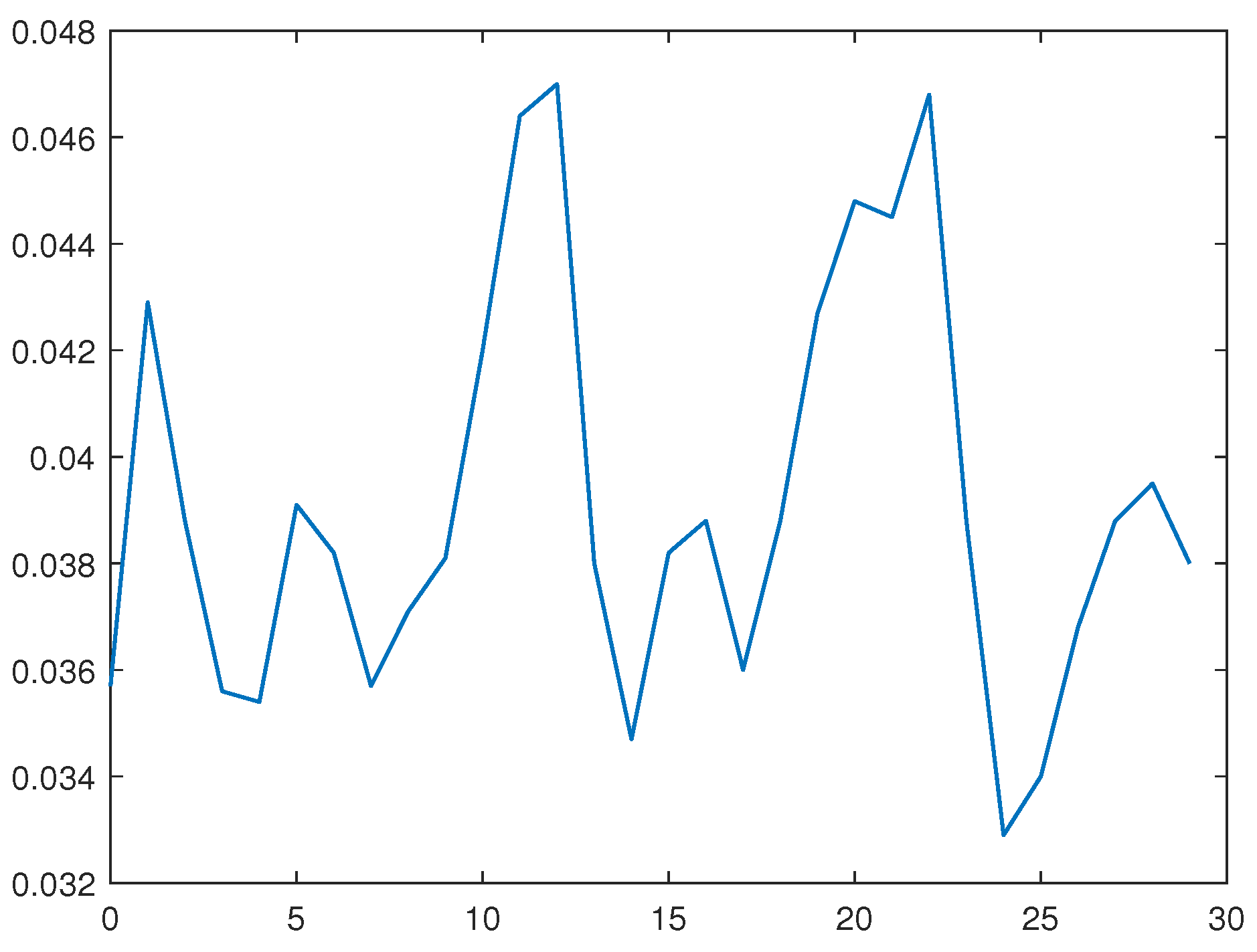
The moment estimate of unknown parameters will be illustrated by some financial data observed from software Wind. Figure 1 graphically depicts the Hibor (Hongkong InterBank Offered Rate) interest rate data from 28 May to 12 July in 2021 (except weekends and holidays), The value of the interest rate fluctuates around 0.038. Assuming that the interest rate follows the general economic behavior of mean reversion, it is acceptable to use Equation (2) to fit the set of data. Thus the estimate for $(\mu ,a,\sigma )$ is obtained from Theorem 5,

$${\mu }^{*}=-0.0044,a^{*}=-0.1204,{\sigma }^{*}=0.1049.$$

Therefore, the interest rate $r_t$ follows the uncertain differential equation

$$\mathrm{d}{r}_t=(-0.0044+0.0212r_t)\mathrm{d}t+0.1049r_t\mathrm{d}{C}_t.$$

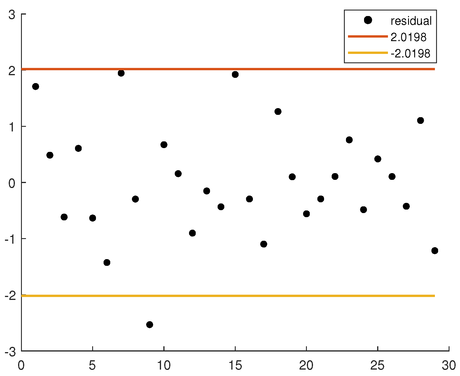
Now we test whether the estimated disturbance term in the uncertain differential equation is appropriate to determine whether it is fitted or not. By substituting the estimates into Equation (4), we can get 29 residuals $h_1({\mu }^{*},a^{*},{\sigma }^{*}),h_2({\mu }^{*},a^{*},{\sigma }^{*}),\cdots ,h_{29}({\mu }^{*},a^{*},{\sigma }^{*})$ as shown in

Table 1. Residuals in the uncertain differential equation.

1.7086	0.4861	−0.6157	0.6073	−0.6340	−1.4259	1.9471	−0.2959	−2.5321	0.6726
0.1565	−0.9019	−0.1516	−0.4336	1.9226	−0.2945	−1.0977	1.2628	0.0998	−0.5581
−0.2930	0.1070	0.7583	−0.4844	0.4193	0.1050	−0.4238	1.1035	−1.2144

. Then we will confirm whether the 29 residuals are samples of $\mathrm{N}$ (0,1) is fit.

Suppose that the residuals are samples of $\mathrm{N}(e,\sigma )$. Then the test for the hypotheses

$$\begin{array}{c}{H}_0:e=0\mathrm{and}\sigma =1\mathrm{versus}{H}_1:e\ne 0\mathrm{or}\sigma \ne 1\hfill \end{array}$$

(6)

at significance level $\alpha =0.05$ is

$$\begin{array}{c}\hfill W=\left\{(z_1,z_2,\cdots ,z_{29}): \mathrm{there\; is\; at\; least} 2 \mathrm{of\; indexs} i^{\prime }s \mathrm{with}\right.\\ \hfill \phantom{=}\left.1\le i\le 29 \mathrm{such\; that} z_i<-2.0198 \mathrm{or} z_i>2.0198.\right\}\end{array}$$

(7)

From Figure 2, we can see that only

$$h_9({\mu }^{*},a^{*},{\sigma }^{*})\notin [-2.0198,2.0198],$$

the vector of 29 observed data do not belong to W. Thus we can conduct that $h_i\sim \mathrm{N}(0,1)$ is acceptable. In other words, the estimated parameter $({\mu }^{*},a^{*},{\sigma }^{*})$ is appropriate.

7. Discussion

The aim of this research was to build a new interest rate model according to uncertain mean-reverting differential equation, and to apply the observed HIBOR data to setimate the unknown parameters in the model. Within the uncertainty theory, the paper investigated the pricing formulas of zero-coupon bond, the interest rate ceiling and floor respectively. Among the process of solving problems, symmetry appeared in mathematical formulations. Then the paper estimated the unknown parameters in the new interest rate model by methods of moments.

By applying the observed HIBOR interest rate data from 28 May to 12 July in 2021 (except weekends and holidays) in the new model, the following uncertain differential equation were obtained:

$$\mathrm{d}{r}_t=(-0.0044+0.0212r_t)\mathrm{d}t+0.1049r_t\mathrm{d}{C}_t.$$

Then 29 residuals were calculated by uncertain hypothesis test, only does the 9-th residual not belong to interval $[-2.0198,2.0198]$, the uncertain model is a good fit to the observed data. Finally, according to the uncertain interest rate model, the forecast uncertain variable and the 95 percent confidence interval of HIBOR interest rate on the next work day can be calculated in the future work.

8. Conclusions

In the work, zero-coupon bond, interest rate ceiling and interest rate floor pricing problems based on uncertain mean-reverting differential equation are derived. Furthermore, the moment estimations for unknown parameters are studied and then applied in the actual financial market which is reliable and valuable.

References

- Merton, R.C. Theory of rational option pricing. Bell J. Econ. Manag. Sci. 1973, 4, 141–183. [Google Scholar] [CrossRef] [Green Version]
- Ho, T.; Lee, S. Term structure movements and pricing interest rate contingent claims. J. Financ. 1986, 5, 1011–1029. [Google Scholar] [CrossRef]
- Vasicek, O. An equilibrium characterization of the term structure. J. Financ. Quant. Anal. 1977, 12, 177–188. [Google Scholar] [CrossRef]
- Cox, J.; Ingersoll, J.; Ross, S. An intertemporal general equilibrium model of asset prices. Econometrica 1985, 53, 363–382. [Google Scholar] [CrossRef] [Green Version]
- Liu, B. Uncertainty Theory, 2nd ed.; Springer: Berlin, Germany, 2007. [Google Scholar]
- Liu, B. Fuzzy process, hybrid process and uncertain process. J. Uncertain Syst. 2008, 1, 3–16. [Google Scholar]
- Chen, X.; Liu, B. Existence and uniqueness theorem for uncertain differential equations. Fuzzy Optim. Decis. Mak. 2010, 9, 69–81. [Google Scholar] [CrossRef]
- Gao, Y. Existence and uniqueness theorem on uncertain differential equations with local Lipschitz condition. J. Uncertain Syst. 2012, 6, 223–232. [Google Scholar]
- Yao, K.; Chen, X. A numerical method for solving uncertain differential equations. J. Intell. Fuzzy Syst. 2013, 25, 825–832. [Google Scholar] [CrossRef]
- Yao, K.; Liu, B. Parameter estimation in uncertain differential equations. Fuzzy Optimation Decis. Mak. 2020, 19, 1–12. [Google Scholar] [CrossRef]
- Liu, Z. Generalized moment estimation for uncertain differential equations. Appl. Math. Comput. 2021, 392, 125724. [Google Scholar] [CrossRef]
- Sheng, Y.; Yao, K.; Chen, X. Least squares estimation in uncertain differential equations. IEEE Trans. Fuzzy Syst. 2020, 28, 2651–2655. [Google Scholar] [CrossRef]
- Liu, Y.; Liu, B. Estimating unknown parameters in uncertain differential equation by maximum likelihood estimation. Soft Comput. 2022, 26, 2773–2780. [Google Scholar] [CrossRef]
- Yang, X.F.; Liu, Y.H.; Park, G.K. Parameter estimation of uncertain differential equation with application to financial market. Chaos Solitons Fractals 2020, 139, 110026. [Google Scholar] [CrossRef]
- Ye, T.; Liu, B. Uncertain hypothesis test with application to uncertain regression analysis. Fuzzy Optim. Decis. Mak. 2021, 21, 157–174. [Google Scholar] [CrossRef]
- Liu, B. Some research problems in uncertainty theory. J. Uncertain Syst. 2009, 3, 3–10. [Google Scholar]
- Chen, X. American option pricing formula for uncertain financial market. Int. J. Oper. Res. 2011, 8, 32–37. [Google Scholar]
- Peng, J.; Yao, K. A new option pricing model for stocks in uncertainty markets. Int. J. Oper. Res. 2013, 12, 53–64. [Google Scholar]
- Chen, X.; Liu, Y.; Ralescu, D. Uncertain stock model with periodic dividends. Fuzzy Optim. Decis. Mak. 2013, 12, 111–123. [Google Scholar] [CrossRef]
- Yu, X. A stock model with jumps for uncertain markets. Int. J. Uncertain. Fuzziness Knowl.-Based Syst. 2012, 20, 421–432. [Google Scholar] [CrossRef]
- Dai, L.; Fu, Z.; Huang, Z. Option pricing formulas for uncertain financial market based on the exponential Ornstein-Uhlenbeck model. J. Intell. Manuf. 2017, 28, 597–604. [Google Scholar] [CrossRef]
- Chen, X.; Gao, J. Uncertain term structure model of interest rate. Soft Comput. 2013, 17, 597–604. [Google Scholar] [CrossRef]
- Zhang, Z.; Ralescu, D.; Liu, W. Valuation of interest rate ceiling and floor in uncertain financial market. Fuzzy Optim. Decis. Mak. 2016, 15, 139–154. [Google Scholar] [CrossRef]
- Jiao, D.; Yao, K. An interest rate model in uncertain environment. Soft Comput. 2015, 19, 775–780. [Google Scholar] [CrossRef]
- Sun, Y.; Yao, K.; Fu, Z. Interest rate model in uncertain environment based on exponential Ornstein-Uhlenbeck equation. Soft Comput. 2018, 22, 465–475. [Google Scholar] [CrossRef]
- Zhu, Y. Uncertain fractional differential equations and an interest rate model. Math. Methods Appl. Sci. 2015, 38, 3359–3368. [Google Scholar] [CrossRef]
- Brennan, M.; Schwartz, E. Analyzing convertible bonds. J. Financ. Quant. Anal. 1980, 15, 907–929. [Google Scholar] [CrossRef]
- Yao, K. Uncertain Differential Equations; Springer: Berlin, Germany, 2016. [Google Scholar]
Figure 1.
Actual observations of interest rate.
Figure 2.
Residuals plot.