
System Resilience Evaluation and Optimization Considering Epistemic Uncertainty


1
School of Reliability and Systems Engineering, Beihang University, Beijing 100191, China
2
Science and Technology on Reliability and Environmental Engineering Laboratory, Beijing 100191, China
*
Author to whom correspondence should be addressed.
Symmetry 2022, 14(6), 1182; https://0-doi-org.brum.beds.ac.uk/10.3390/sym14061182
Submission received: 2 May 2022
/
Revised: 25 May 2022
/
Accepted: 5 June 2022
/
Published: 8 June 2022
(This article belongs to the Special Issue Uncertainty Theory: Symmetry and Applications)
Abstract
:Epistemic uncertainties, caused by data asymmetry and deficiencies, exist in resilience evaluation. Especially in the system design process, it is difficult to obtain enough data for system resilience evaluation and improvement. Mathematics methods, such as evidence theory and Bayesian theory, have been used in the resilience evaluation for systems with epistemic uncertainty. However, these methods are based on subjective information and may lead to an interval expansion problem in the calculation. Therefore, the problem of how to quantify epistemic uncertainty in the resilience evaluation is not well solved. In this paper, we propose a new resilience measure based on uncertainty theory, a new branch of mathematics that is viewed as appropriate for modeling epistemic uncertainty. In our method, resilience is defined as an uncertainty measure that is the belief degree of a system’s behavior after disruptions that can achieve the predetermined goal. Then, a resilience evaluation method is provided based on the operation law in uncertainty theory. To design a resilient system, an uncertain programming model is given, and a genetic algorithm is applied to find an optimal design to develop a resilient system with the minimal cost. Finally, road networks are used as a case study. The results show that our method can effectively reduce cost and ensure network resilience.
1. Introduction
In the engineering field, resilience reflects the ability of a system to withstand, adapt, and recover from disruptions (including both external disturbances and internal failures) [1]. If the impact of a disturbance cannot be effectively controlled, the disturbance may cause severe economic or other losses. For example, Hines et al. [2] pointed out that in the past 100 years, North America suffered power losses of as much as 186,000 MW due to natural disasters. Hurricane Isabel devastated the transportation system of the Hampton Roads, VA, region in 2003 and overwhelmed the emergency response system [3]. Besides these direct damages, MacKenzie et al. [4] analyzed the indirect production losses caused by disabled production facilities in the earthquake and tsunami that struck Japan on 11 March 2011. Hence, to reduce the direct and derived damages caused by disruption, more and more researchers begin to focus on system resilience evaluation and improvement. Resilience has become a hot research topic.
Many researchers have proposed a resilience definition from different views. Bruneau et al. [5] defined seismic resilience as the ability of systems to mitigate hazard, contain effects, and carry out recovery activities. Arcuri et al. [6] analyzed resilience on healthcare systems. They pointed out that healthcare system resilience has been linked to sustainability, safety, quality, and adaptive capacity. Cook and Long [7] studied the adaptive capacity in organization resilience. They proposed that the ability to borrow and adjust an adaptive capacity are features of resilience system and resilience engineering. Woods [8] proposed four senses of resilience including rebound, robustness, extensibility, and adaptability. Jain et al. [9] defined resilience as three abilities: avoidance, survival, and recovery. Pawar et al. [10] summarized resilience definitions and proposed that the resilience of industrial systems have three common themes, i.e., absorption, adaptation, and restoration. The same view can also be seen in Abbasnejadfard et al. [11].
To evaluate system resilience, researchers have proposed many measures, which can be categorized as deterministic and probabilistic measures. Deterministic resilience measures and compares a system’s behavior before and after a certain disruption, and typical deterministic resilience measure methods include the resilience loss [5], performance integral ratio-based measures [1,12,13,14], recovered performance ratio-based measures [15], and performance loss rate-based measures [16,17,18], etc. Probabilistic resilience measures consider the randomness of both a disturbance and the system response to it, and typical probabilistic resilience measures include deterministic resilience distribution-based measures [19], and performance degradation and recovery time-based measures [5,20,21], etc. Using the resilience measures described above, system resilience was evaluated using real data and simulations. Roach et al. (2018) [22] developed ten other metrics to evaluate the resilience of a water resources system with real data. Roberto and Patelli (2018) [23] simulated the perfor mance of a power grid system after disruptions and evaluated its resilience. Other researchers designed system resilience strategies such as protection strategies [24], reconfiguration strategies [25], and recovery strategies [26]. To design a resilient system, resilience optimization models and algorithms were also developed. For example, Li et al. [27] proposed a resilience optimization model to find the best recovery strategy for road networks after disruptions. Miller et al. [28] proposed a network resilience optimization model to find the optimal recovery strategy for a rail-based intermodal container network considering the uncertainty of traffic flow. Zhang et al. [29] proposed a resilience optimization model for road networks to find the best structure for a resilient road network. Salas and Yepes [30] proposed an improved planning support system to afford a planning alternative over the Spanish road network. Their method proved that decentralization optimization can improve the adaptive capacity of road networks and then improve resilience.
However, these resilience measures and their evaluation and optimization methods have problems when epistemic uncertainty existed. Epistemic uncertainty describes the subjective uncertainty caused by insufficient knowledge and information. In the system design process, no operation data can be obtained, and designers can only conduct tests or simulations to observe how disruptions affect a system. As is generally known, it is both time consuming and costly to conduct tests or simulations, especially for large-scale systems, so only limited data can be obtained. Due to this data insufficiency, the law of resilience cannot be obtained, which may lead to a poor knowledge of system resilience. In this situation, it is necessary to rely on empirical data to make decisions. When experts are investigated for empirical data, empirical data are asymmetrical due to the difference of knowledge between experts. To conclude, researchers face the problems of data insufficiency [31], poor knowledge of a system [32,33], and data asymmetry [34]. In this stage, the resilience evaluation for a new system is a typical problem with epistemic uncertainty that differs from traditional aleatory uncertainty [33,35]. Most existing resilience measures only consider aleatory uncertainty, i.e., the dispersion of both a disturbance and a system response to it. A few researchers have already studied epistemic uncertainty, and applied Bayesian theory [36] and evidence theory [37] to quantify the epistemic uncertainty of performance degradation and the disruption intensity in the resilience process, however, evidence theory will lead to the interval expansion problem for large systems [38], and Bayesian theory will bring subjective information into probability theory. There is no evidence to prove that subjective probability follows the operation law of probability theory [38,39,40]. Due to the reasons listed above, the problem of determining how to quantify epistemic uncertainty in resilience evaluation has not been well solved. The uncertainty theory proposed by Liu [41], a new branch of axiomatic mathematics, provides another solution for the epistemic uncertainty quantification problem, and this theory has been successfully applied in engineering. Hu et al. [42] applied uncertainty theory into risk assessment. Kang et al. [43] combined the reliability with uncertainty theory. Yang et al. [34] used uncertainty theory to measure epistemic uncertainty in spare parts transportation optimization. Li et al. [44] proposed a reliability analysis method for a muti-state deteriorating system based on belief reliability theory. These studies showed that compared with other methods for epistemic uncertainty, such as fuzzy theory, interval theory, and evidence theory, uncertainty theory is more applicable in epistemic quantification.
This paper proposes an uncertainty theory-based resilience measure and provides both resilience evaluation and optimization methods. Our main contributions are as follows:
- A new uncertainty theory-based resilience measure is proposed to quantify the epistemic uncertainty in resilience evaluation. Compared with other methods, our new resilience measure has a solid mathematical foundation in epistemic quantification;
- A resilience evaluation framework is provided for the new resilience measure. By building the performance model and the disruption response model, and obtaining the distribution function of uncertain variables, the distribution function of the disruption response can be calculated, and the system resilience can be evaluated;
- To build a resilient system with a minimum budget, an uncertain programming model is given and a genetic algorithm is applied to solve the optimization problem. A road network case verifies the effectiveness of our new model and algorithm.
The remainder of this paper is organized as follows. Section 2 gives a brief introduction of both resilience and uncertainty theory. Section 3 proposes our uncertainty theory-based resilience measure. Section 4 provides both resilience evaluation and optimization methods. Section 5 describes the application of two road networks as case studies to verify the effectiveness of our methods. Finally, concluding remarks are provided in Section 6.
2. Basic Concepts and Theories
2.1. System Response after Disruptions
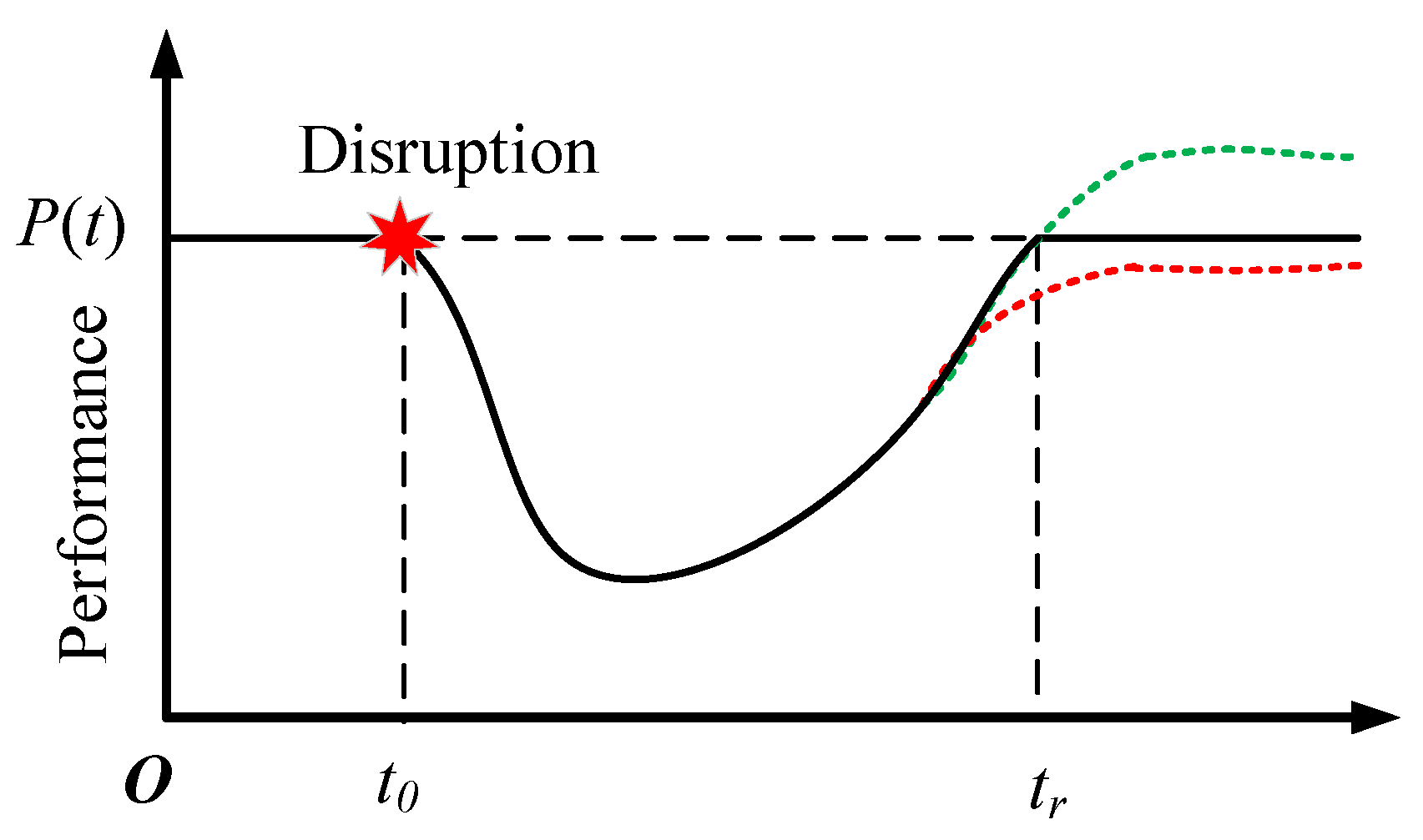
After a disruption occurs, the system performance may degrade and then recover due to the implementation of recovery activities. This performance change process (i.e., the system response) after a disruption is shown in Figure 1. Some performance change processes are gradual and continuous, as Figure 1 shows, and some are discrete with sudden changes. In this figure, the system performed steadily at the beginning and suffered a disruption at time . Then, the system performance started to decrease. After taking some recovery actions, the system performance gradually returns back. In some cases, the system may finally reach a better performance with resource reconfiguration, and also may get a worse performance as the system cannot recover completely. Considering that the ability of system to withstand, adapt, and recover from disruptions can be reflected in the performance changing process, many resilience measures are proposed based on the system’s response to the disruption.
2.2. Uncertainty Theory
Uncertainty theory is a new branch of axiomatic mathematics. In uncertainty theory, the belief degrees of events are quantified by defining the uncertain measure. Some basic concepts and results for uncertainty theory are presented as follows.
Definition 1
(Uncertain Measure [41]). Letting be a nonempty set and be a -algebra over , each element in is an event. A set function is called an uncertain measure if it satisfies the following axioms.
Axiom 1
(Normality Axiom). for the universal set .
Axiom 2
(Duality Axiom). for any event , where is the complementary set of .
Axiom 3
(Subadditivity Axiom). For every countable sequence of events , there is
Axiom 4
Definition 2
(Uncertain Variable [41]). An uncertain variable is a function from an uncertainty space for the set of real numbers such that is an event for any Borel set of real numbers.
Definition 3
(Uncertainty Distribution [41]). The uncertainty distribution of an uncertain variable is defined by
for any real number .
Definition 4
(Regular Uncertainty Distribution [46]). An uncertainty distribution is said to be regular if it is a continuous and strictly increasing function with respect to for which , and
Definition 5
(Inverse Uncertainty Distribution [46]). Letting be an uncertain variable with a regular uncertainty distribution , then the inverse function is called the inverse uncertainty distribution of .
Definition 6
(Independence [45]). The uncertain variables are said to be independent if
for any Borel sets of real numbers.
Definition 7
(Strictly Monotone Function of Uncertain Variables [46]). A real-valued function is said to be strictly monotone if it is strictly increasing with respect to and strictly decreasing with respect to ; that is
whenever for and for , and
whenever for and for .
Theorem 1
(Operational Law: Inverse Distribution [46]). Letting be independent uncertain variables with regular uncertainty distributions respectively, if is a continuous and strictly increasing with respect to and strictly decreasing with respect to , then
has an inverse uncertainty distribution
3. Uncertainty Theory-Based Resilience Measure
We first define the uncertainty theory-based resilience as follows.
Definition 8
(Resilience). Letting a system state variable be an uncertain variable that refers to the system’s state after disruption and letting be the resilience domain of the system state, then the resilience is defined as the belief degree that the system’s state after disruption is within the resilience domain, i.e.,
where refers to the system’s state after disruption, and it can be described by the system’s behavior after the disruption.
This resilience measure is a general one, and it describes the chance that the system’s resilience is satisfactory for user requirements. Because most existing research uses a system’s performance change process to reflect the system’s behavior after disruption, we also define the state variable based on this. Let the system’s response to the disruption be a state variable and denote its threshold as . Then, the event can be recorded as , and the resilience can be measured as:
In our paper, the average performance after disruption is selected to reflect the system’s response to the disruption event. It is called the disruption response and can be calculated as [1]
where is the time at which the disruption occurs, is the maximum allowable recovery time determined by users, and is the normalized performance of the system after the disruption. Using the min-max method [47], can be calculated as
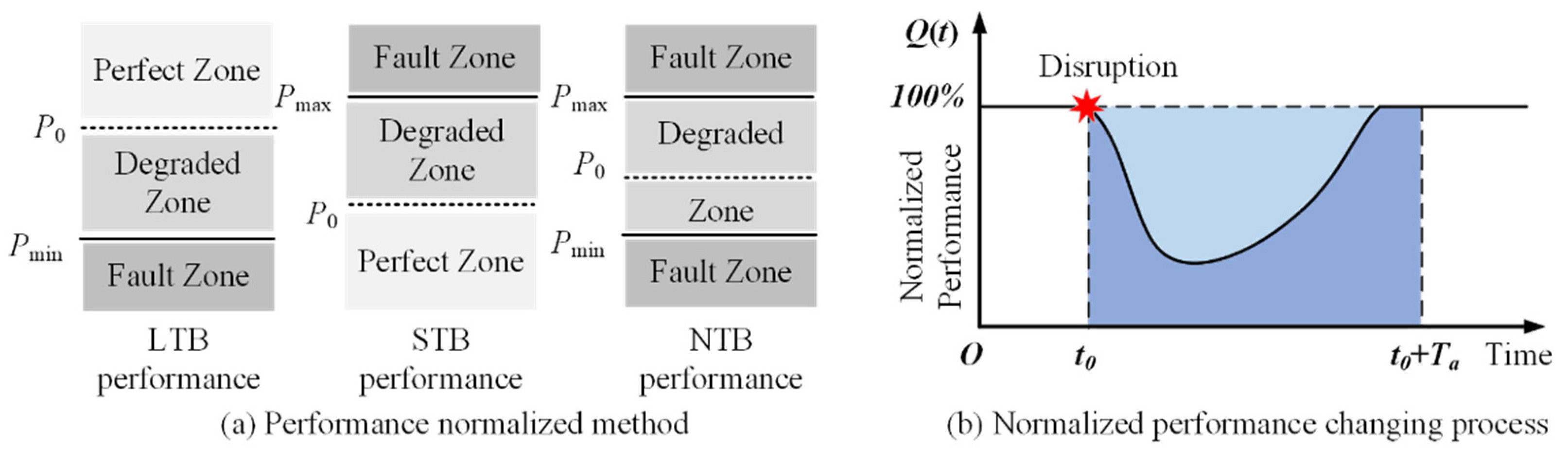
where is the performance of the system without disruption, and and are the minimum acceptable value and the maximum acceptable value of the system performance , respectively. Once the performance exceeds and , the system cannot be used completely. Here, LTB means the larger-the-better, and this is true for the system functions when . STB means the smaller-the-better, and this is true for the system functions when . NTB means the more nominal-the-better, and this is true for the system functions when . The physical meaning of our normalized method is shown in Figure 2a. Using the performance normalization method in Equation (13), the performance in the perfect zone of Figure 2a are normalized as , those in the fault zone are normalized as , and those in the degraded zone are normalized as the percentage of the performance that the system can provide.
Figure 2b shows a normalized performance change process, and can be calculated using the ratio of the area of the dark blue zone to the areas of both the dark blue and the light blue zones. is a comprehensive index including robustness, adaption, and recovery capability. Its physical meaning is the average normalized performance in the maximum allowable recovery time after a disruption. The event means that the system’s average performance after the disruption is within the resilience domain. In this way, our new resilience measure quantifies the belief degree of the system’s behavior meeting the requirements after disruptions.
According to uncertainty theory, is an uncertain variable. Letting be the distribution of , our new resilience measure can be calculated as
After the actual or experimental data are obtained, researchers can use uncertainty statistics to obtain the distribution function and calculate the resilience within the threshold .
4. Resilience Evaluation and Optimization
In this section, we provide a resilience evaluation framework first, and then we propose a resilience optimization method to assist with the system’s resilience design.
4.1. Resilience Evaluation
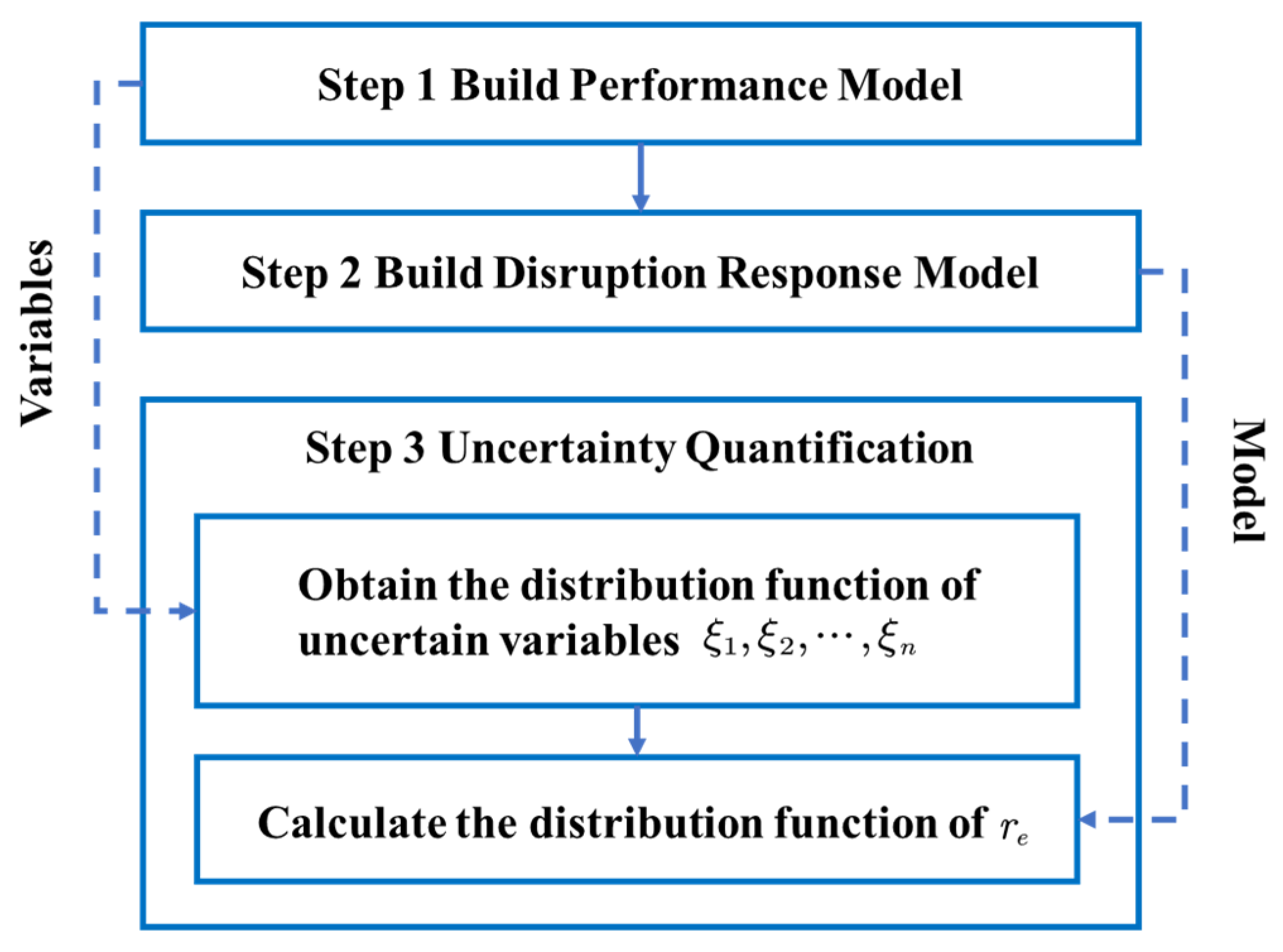
Based on the resilience definition given above, a resilience evaluation framework is proposed as shown in Figure 3. The resilience evaluation steps are as follows.
Step 1: The performance model is built to describe the system’s performance change over time. The general performance model is as follows:
where is the system performance at time , and the function is the performance model. It is worth noting that in this paper we focus on the performance changing process of a system after disruption, and disruption modeling and generation will be our future work. Therefore, are parameters that describe the performance characteristics such as the performance degradation and recovery time. These parameters differ in different resilience processes. In this paper, parameters are uncertain variables. With performance changing process data after several disruption events, the distribution functions of can be obtained by an uncertain statistic method. Here, we assume that are independent uncertain variables. This limitation will be overcome in future work.
Step 2: The disruption response model is built to calculate that is defined in Equation (12). The general form of the disruption response model can be denoted as:
where is the disruption response model. It can be calculated by substituting Equation (15) into Equations (12) and (13). According to the definition of in Equation (12), this model can be used to calculate the average value of a system’s normalized performance during a performance changing process. Here the disruption response model is a deterministic model. As described in Step 1, parameters are uncertain variables. Therefore, the disruption response is also an uncertain variable. Its distribution function can be obtained based on the distribution functions of and the operation law of uncertain theory.
Step 3: The uncertainty quantification is determined. As described in Section 3, resilience is defined as an uncertain measure, and it can be explained as the quantification of the uncertainty of a system’s disruption response. After building the disruption response model, the system resilience can be obtained based on the distribution function of the parameters in the model. Therefore, the uncertainty quantification can be divided into two sub-steps:
- The distribution function of is calculated. Using the distribution function of the uncertain variables , the resilience can be evaluated using Equation (14). According to Theorem 1, the distribution function of can be calculated as follows.
It is assumed that (1) the disruption response function is continuous and strictly increasing with respect to and strictly decreasing with respect to , and (2) the independent uncertain variables have the regular uncertainty distributions . Then the disruption response has the inverse uncertainty distribution
where is the belief degree, and is the inverse distribution of the disruption response. The monotonicity of can be analyzed according to the physical meaning of parameters and .
Based on the inverse distribution of the disruption response in Equation (17), the 99-method [46] can be used to obtain the distribution function of the disruption response, and then the system resilience can be calculated.
4.2. Resilience Optimization
A resilience optimization method is proposed to find the optimal system design. In this research, resilience is defined as an uncertain measure, and the resilience-based optimization model is an uncertain programming model. In 2009, Liu [50] proposed the theory of uncertain programming, and provided the basic models for the uncertain programming and optimization methods. Based on conclusions from that research, the steps of our optimization method are as follows.
4.2.1. Optimization Model
Many resilience-based models have been provided in previous studies. For example, Zhang et al. [29] proposed a resilience-based network optimization model with the aims of finding the minimum cost design with the resilience constraint. Based on the same idea, our optimization model is as follows:
where the function is the system design cost, is the system resilience, is the resilience requirement, and is the vector of the optimization variable, which is determined by the system design. Equation (18) only accounts for the cost and resilience of the system, and researchers can add other constraints as needed for practical problems.
4.2.2. Optimization Model Transformation
Liu [50] proved that the uncertain programming model could be transformed into a crisp mathematical programming model according to the operation laws in uncertainty theory. According to Theorem 1, the constraint function in Equation (18) is equivalent to crisp mathematical programming
where are inverse uncertain distributions of .
4.2.3. Optimization Method
To solve the crisp mathematical programming shown in Equation (19), common optimization algorithms such as the gradient descent method and the Hessian matrix method can be used. For some complex optimization problems, intelligent algorithms such as genetic algorithms and particle swarm optimization algorithms are better choices.
5. Case Study
We use two road network cases to demonstrate the application of our resilience evaluation and optimization method.
5.1. Case Introduction
Case 1: A road network with a simple structure is shown in Figure 4. This case is taken from Hiller et al. [51]. Nodes S and T are the source and destination nodes, respectively. In the figure, the numbers in the brackets represent the link number and the capacity. The maximum flow between Nodes S and T is chosen as the key performance parameter of the system. This model represents a determinate situation, in which the network topology is deterministic.
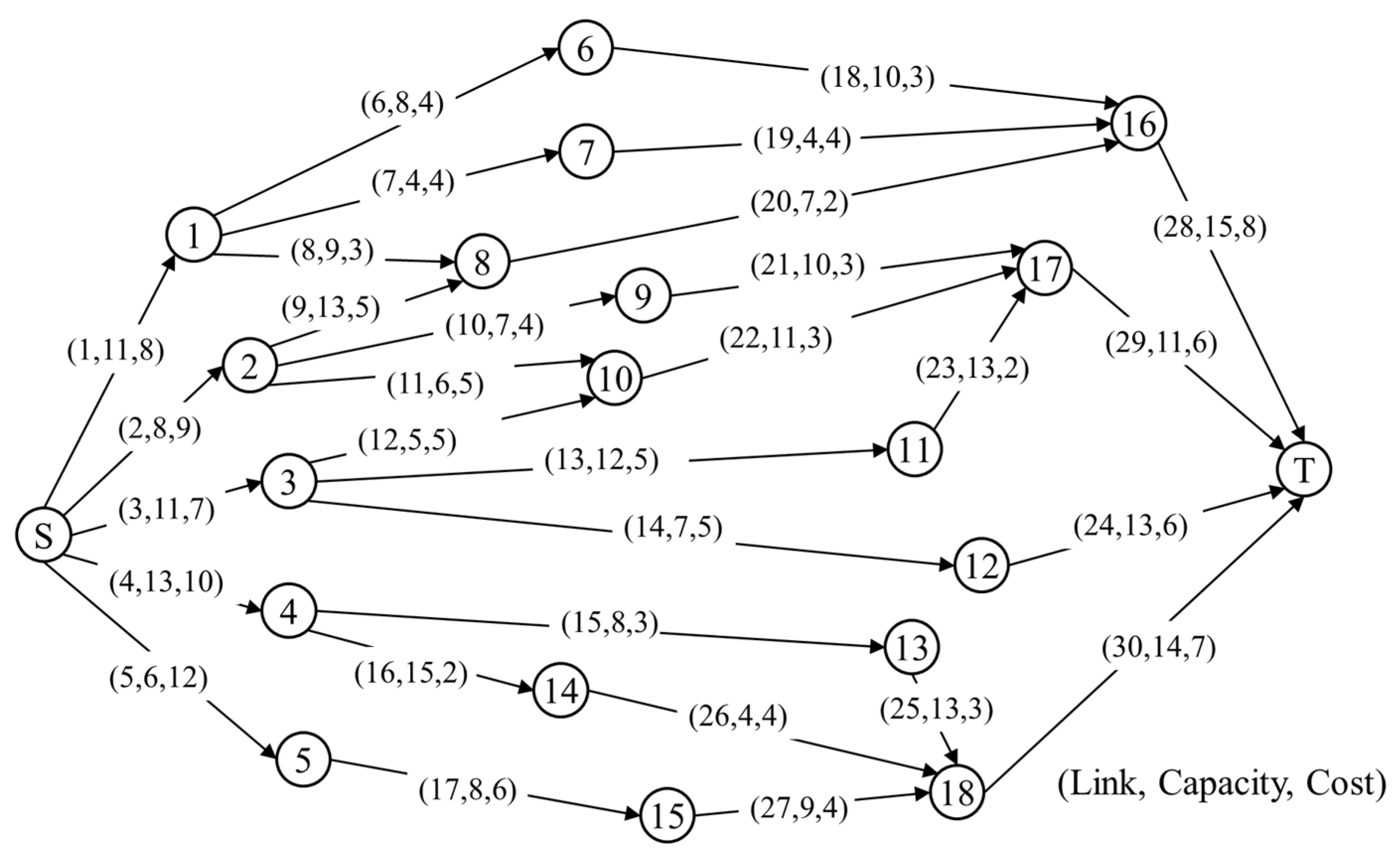
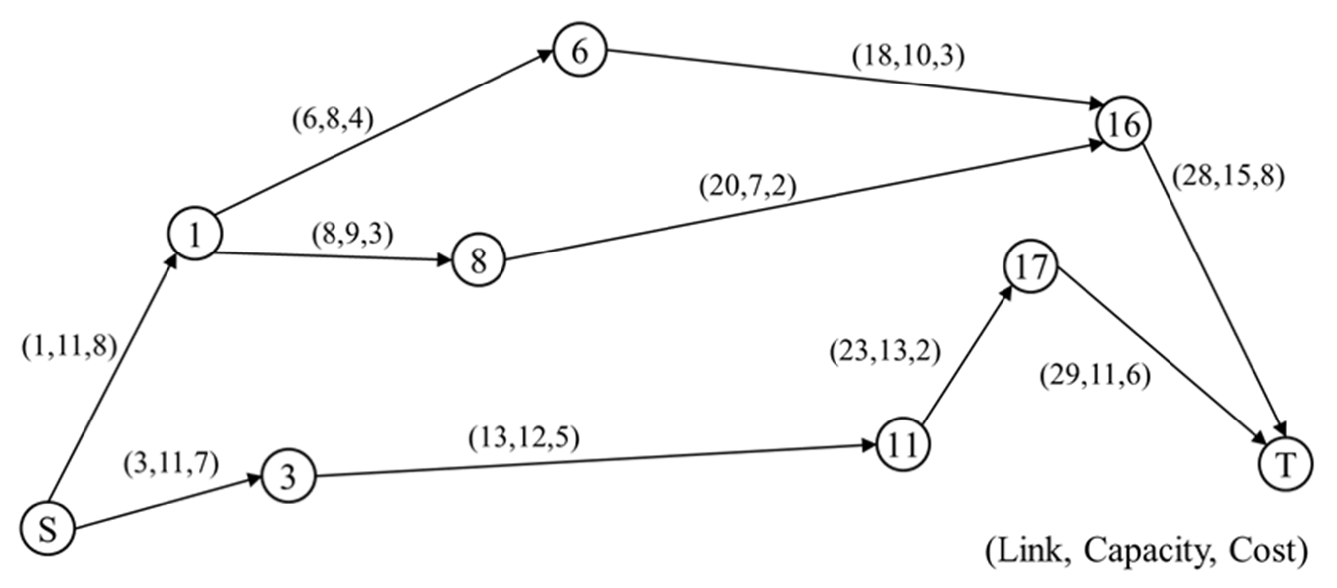
Case 2: Figure 5 illustrates another road network with a slightly more complex structure. This case is taken from Dai and Poh [52]. In this problem, all of the links represent potential roads. Designers need to find an optimal road network design that minimizes the costs within the constraint of the system resilience. Similar to Case 1, the maximum flow between Nodes S and T is selected as the key performance parameter. The numbers in the brackets represent the number, capacity, and cost of the links.
To simplify the problem, we make the following assumptions:
- Only one link is affected during each disruption;
- The capacity of the road links degrades suddenly after disruptions, and the capacity recovery processes are linear processes. This is a widely used assumption in resilience research [53]. In most disruptions, especially natural disasters and traffic accidents, the road link capacity degradation time is very short, and the capacity degradation time can be regarded as zero;
- The uncertain variable follows a linear uncertain distribution as followswhere is the distribution function of the maximum performance degradation ;
- The uncertain variable follows a lognormal uncertain distribution as followswhere is the distribution function of the recovery time , and and are the expected value and the standard deviation of the normal uncertainty distribution, respectively.
5.2. Case 1: Road Network Resilience Evaluation
5.2.1. Resilience Evaluation
Using the resilience evaluation method proposed in Section 4.1, the resilience of the road network in Case 1 is evaluated as follows.
(1) The system performance model is built. In this case, the maximum flow between Nodes S and T is determined by the capacity of the road link. Therefore, the system performance model should be built based on the road link capacity disruption model and the correlation between the road link capacity and the maximum flow.
After a certain disruption, the capacity of road link i at time t can be expressed as
where is the capacity of road link in the normal state, is the maximum capacity degradation of link , and is the recovery time of link .
For linear capacity recovery processes, can be written as follows:
After the disruption, the maximum flow can be calculated according to the capacity of the road links as
where .
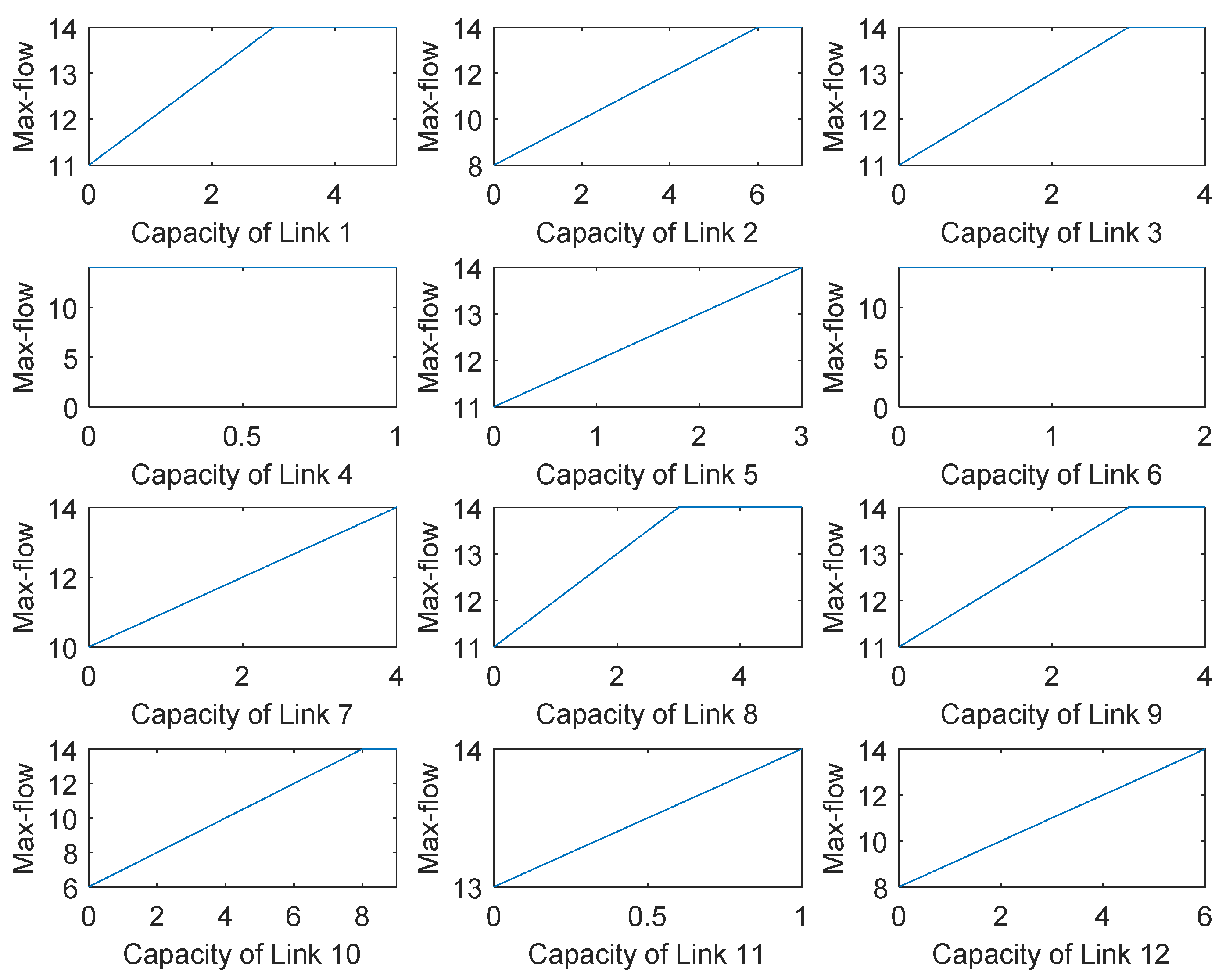
Obviously, the function in Equation (22) is a piecewise linear function with two sections, as shown in Figure 6. In this case, the disruption of link affects the maximum flow as follows:
where is the inflection point of the piecewise linear function for link , which is determined by the network structure. Figure 6 shows how the capacity of each link affects the maximum flow, and the values for the parameters and are shown in Table 1.
(2) The disruption response model is built. In this case, the maximum flow is an LTB parameter. According to the performance normalization method given in Equation (13), the normalized maximum flow can be calculated as:
where , .
Combining Equations (23) and (26), the normalized maximum flow of the network is as follows:
Taking Link 1 as an example, the normalized maximum flow of the network when Link 1 is disrupted is as follows:
According to Equation (12), the disruption response of the network can be calculated as follows:
(3) The uncertainty is quantified. In this case, and are uncertain variables. Taking Link 1 as an example, let , , and , so the inverse distributions of the variables are as follows:
where is a belief degree between 0 and 1.
After the distribution functions of the uncertain variables are obtained, the inverse distribution function of the network disruption response can be computed using Equation (17). According to the physical meanings of , , and , it is obvious that is continuous and strictly decreasing with respect to and . Letting , the inverse distribution of when Link 1 is disrupted can be expressed as follows:
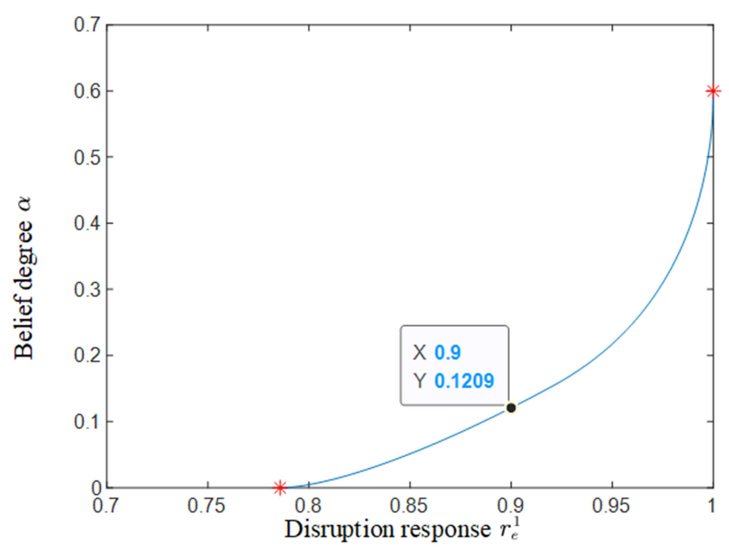
As Equation (32) shows, the inverse distribution function of is complex. Using the linear interpolation method, the distribution function of when Link 1 is disrupted can be obtained, as shown in Figure 7. According to Equation (14), letting , the resilience when Link 1 is disrupted can be calculated as
From Figure 7, one can see that:
- The belief degree of the event is 0. It is obvious that the value of the network resilience is at a minimum when Link 1 is totally interrupted and cannot recover. In this situation, the maximum flow after the disruption has a constant value of 11. can also be calculated using the ratio of 11 to 14, and is equal to 0.7857;
- The belief degree of the event is 0.6. According to the network structure, the maximum flow of the road network starts to decrease only when the capacity degradation of Link 1 exceeds two. According to Equation (20), the belief degree of the event is 0.6.
The two results are intuitive when Link 1 is disrupted, and the effectiveness of our method is verified.
5.2.2. Results and Discussion
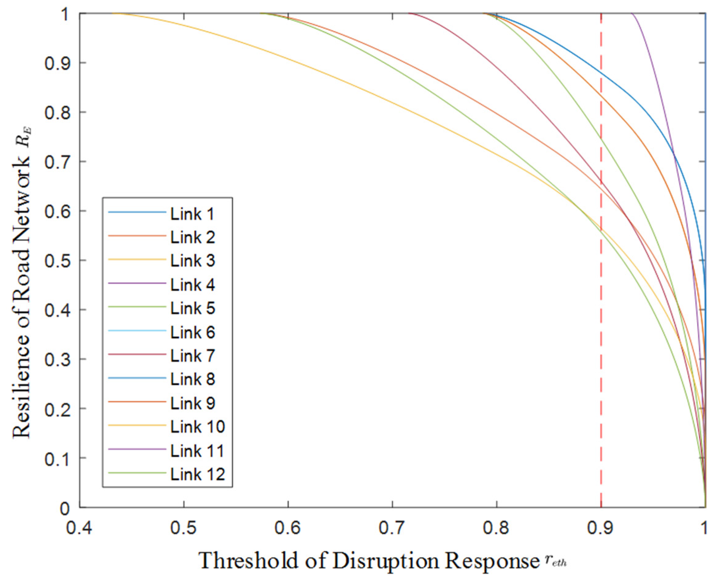
Using the same method, the network resilience when each link is disturbed is evaluated. Letting , the system resiliencies when different links are disturbed are shown in Table 2.
As shown in Table 2, the network resilience is equal to one when Links 4, 6, and 11 are disturbed. Links 4 and 6 are redundant road links, and the system operates normally even if Links 4 and 6 fail completely. If Link 11 completely fails and cannot recover, is 0.9286 (ratio of maximum flow when Link 11 completely fails to the initial max-flow), i.e., is always larger than 0.9, and it is always in the resilience domain.
Figure 8 further illustrates how the system resilience varies with when different links are disturbed.
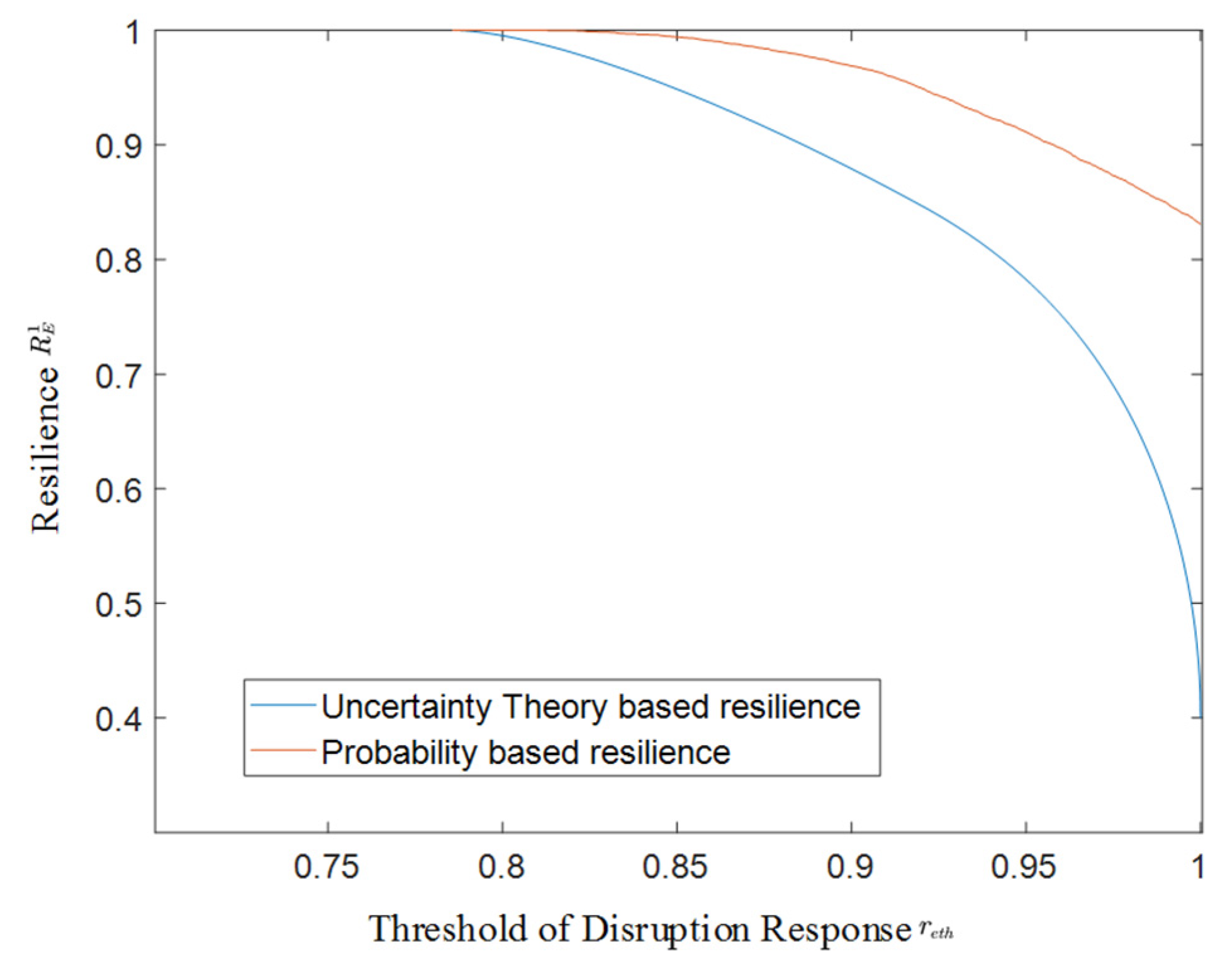
To highlight the novelty of our method, we compared our resilience evaluation result with a probability-based measure. The probability-based measure is defined as
where is the probability measure, is the probability-based resilience measure when Link 1 is disrupted. can be calculated using the Monte Carlo method.
The resilience evaluation result is shown in Figure 9.
As is shown in Figure 9, the uncertainty theory-based resilience evaluation result is always less then probability-based resilience. This result shows the advantage of our new resilience measure. When epistemic uncertainty exists, our measure can provide a more conservative result, which is beneficial to decision makers. Similar results can also be found in [44].
5.3. Case 2: Road Network Resilience Optimization
5.3.1. Network Optimization
According to the resilience optimization method in Section 4.2, the road network in Case 2 is optimized as follows.
(1) The optimization model is built. In this case, the network cost is regarded as the optimization goal, and the cost function can be expressed as
where is the cost of the network, is the cost of link , is a binary decision variable, and
Our network should provide enough transportation and network resilience. The requirement of the transportation amount can be expressed by an inequality constraint as follows:
where is the maximum flow of the network with a link composition vector , which is a vector of binary decision variables, and is the minimum requirement of the maximum flow.
In this case, the system resilience is regarded as the minimum value of the system resilience when a single link is disrupted. This means that designers care about the worst situation. Ahmadian [54] applied the same resilience measure. The system resilience requirement can be expressed as follows:
where are the system resilience when Links are disrupted. Letting , can be evaluated by using the resilience evaluation methods described in Section 4.1.
It is worth noting that it is probable that not all of the links are included in the optimal solution. However, Equation (37) is still applicable. The reason for this is that if link is not included in the optimal network, the network performance is not be influenced by the disruption to link . is equal to one and does not affect the result of Equation (37).
The optimization model of this case is as follows:
(2) The optimization model is transformed. The resilience constraint in the optimization model of Equation (38) represents the fact that the minimum resilience of the system with different disruptions should be greater than the requirement value. This is equivalent to the event of the resilience of the system with each disruption being greater than the requirement value. Additionally, the resilience constraint is an uncertainty constraint. According to the optimization model transformation method discussed in Section 4.2, the resilience constraint can be transformed as follows
where are the disruption responses of the network when Links are disrupted, are the maximum performance degradations of Links , and are their inverse uncertainty distributions.
In this way, the resilience optimization model given in Equation (38) is equivalent to the crisp mathematical programming, as follows:
(3) The optimization problem is solved. The network structure optimization problem is a 0–1 integer optimization problem, and the genetic algorithm, which is widely used in network resilience research [28,55,56], is used to solve the optimization problem given in Equation(40). In the genetic algorithm, every individual in the population is judged to be a feasible solution or not. However, in practice, varies with the network structure vector and the disruptions to different links. It is inefficient to derive the expressions for with different disruptions for every individual during optimization. To solve the problem, we propose a numerical algorithm to calculate in Equation (40). The Algorithm 1 is as follows.
| Algorithm 1:calculation |
| Input: The sample number N The link capacity The resilience constraint The maximum allowable recovery time Output: The disruption response Step 1 let Calculate the maximum flow when all links are in normal state. Step 2 For to , and calculate the maximum flow at time . Endfor Step 3 |
Using the genetic algorithm, the optimization problem can be solved. The optimization results are discussed in Section 5.3.2.
5.3.2. Results and Discussion
To solve the optimization problem, the related parameters of the optimization model and the genetic algorithm are set as shown in Table 3.
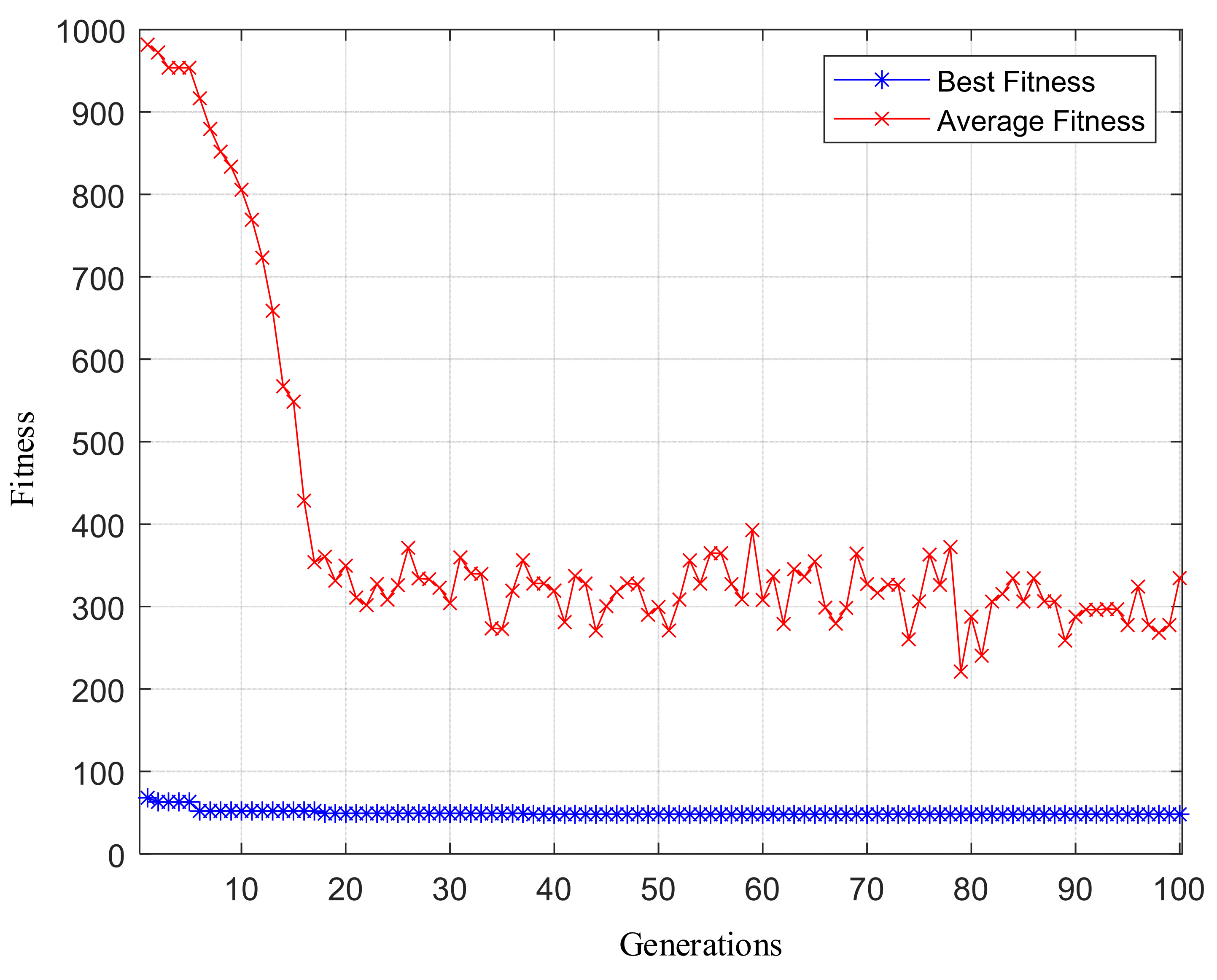
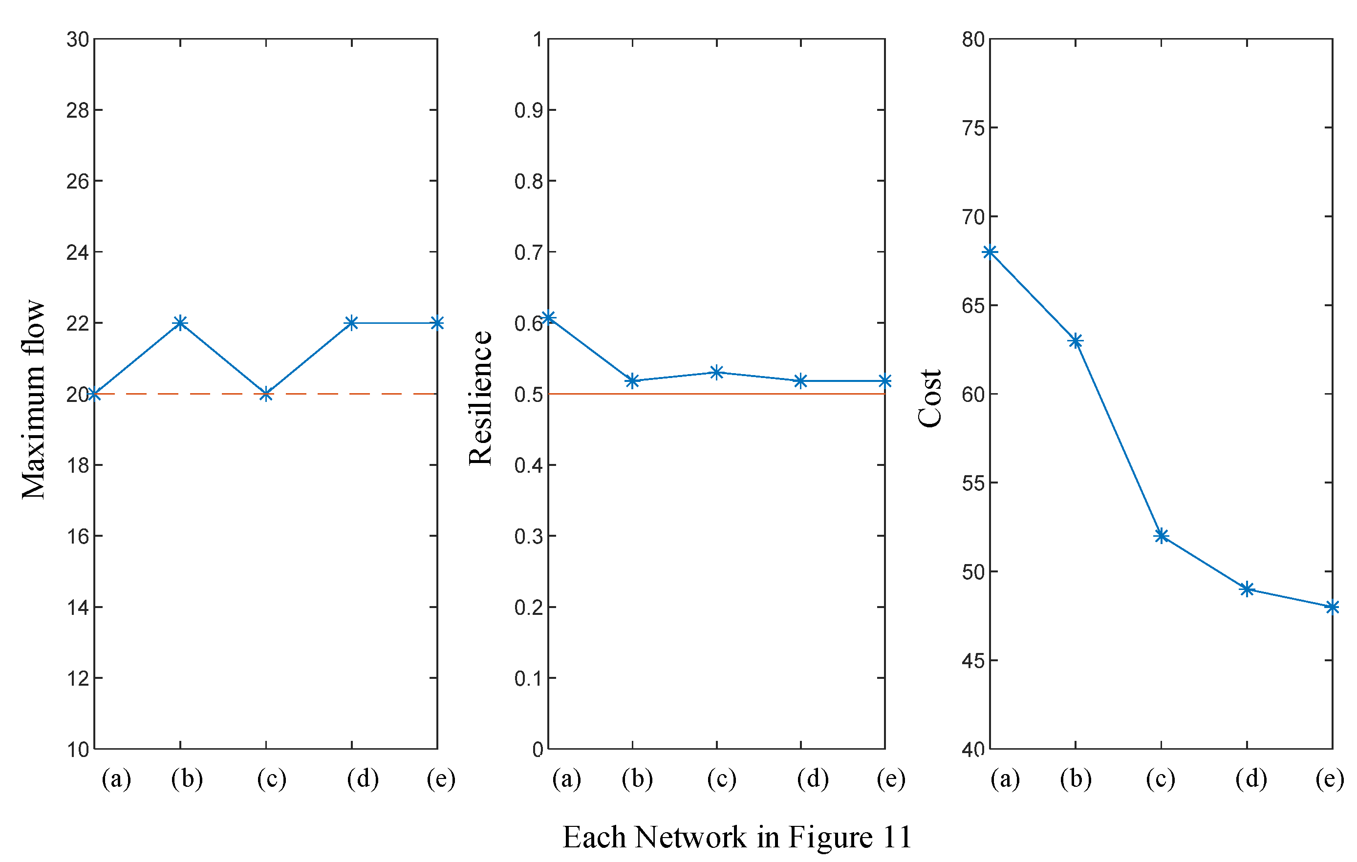
Figure 10 presents the optimization process using the genetic algorithm. With the increase in the generations, both the average and the best fitness of the population increase and are close to a stable value. The evolution process of the optimal network structure in each generation is shown in Figure 11. The resiliencies, maximum flows, and costs of the networks in Figure 11 are shown in Figure 12. The results in Figure 11 and Figure 12 verify that our method can effectively minimize the network cost for both the maximum flow and the resilience constraints.
6. Conclusions
In this study, the uncertainty theory is introduced to quantify the epistemic uncertainties in resilience research. A new uncertainty theory-based resilience measure is proposed based on a system’s response to disruption. Our new resilience measure has a solid mathematical foundation and a clear physical significance. It can be used to evaluate resilience and design a resilient system with insufficient data, such as the system design stage. To evaluate the system resilience, a resilience evaluation framework is proposed, and the framework contains three steps: (1) The system performance model is built; (2) the system’s disruption response model is built; and (3) the uncertainty of the variables in the system performance model and the uncertainty of the disruption response are quantified, and finally the system resilience is calculated. Furthermore, a resilience optimization method is proposed to design a resilient system with minimal costs. Based on the uncertain programming theory, a resilience-based optimization model and a model transmit method are proposed, and intelligent algorithms (e.g., genetic algorithms) can be used to solve this type of optimization problem. Two road networks are used in the case study to verify the effectiveness of our resilience evaluation and optimization method.
In the future, we will apply the uncertain statistics methods to the resilience evaluation and optimization problem. Without assumptions about the distributions of uncertain variables, these methods can be used in real data cases. This method will also be used in multi-scale systems to build a bottom-up resilience evaluation framework.
Author Contributions
Conceptualization, R.K.; methodology, Q.D.; software, Q.D.; validation, Q.D. and R.L.; formal analysis, Q.D.; investigation, Q.D.; writing—original draft preparation, Q.D.; writing—review and editing, R.L.; supervision, R.L. and R.K.; project administration, R.L. and R.K.; funding acquisition, R.L. and R.K. All authors have read and agreed to the published version of the manuscript.
Funding
This research was funded by the National Natural Science Foundation of China (61773044) and National Key Laboratory of Science and Technology on Reliability and Environmental Engineering (WDZC2019601A301).
Institutional Review Board Statement
Not applicable.
Informed Consent Statement
Not applicable.
Data Availability Statement
Not applicable.
Conflicts of Interest
The authors declare no conflict of interest.
References
- Li, R.Y.; Dong, Q.; Jin, C.; Kang, R. A New Resilience Measure for Supply Chain Networks. Sustainability 2017, 9, 144. [Google Scholar] [CrossRef] [Green Version]
- Hines, P.; Apt, J.; Talukdar, S. Large blackouts in North America: Historical trends and policy implications. Energy Policy 2009, 37, 5249–5259. [Google Scholar] [CrossRef]
- Smith, C.M.; Graffeo, C.S. Regional impact of Hurricane Isabel on emergency departments in coastal southeastern Virginia. Acad. Emerg. Med. 2005, 12, 1201–1205. [Google Scholar] [CrossRef]
- MacKenzie, C.A.; Santos, J.R.; Barker, K. Measuring changes in international production from a disruption: Case study of the Japanese earthquake and tsunami. Int. J. Prod. Econ. 2012, 138, 293–302. [Google Scholar] [CrossRef]
- Bruneau, M.; Chang, S.E.; Eguchi, R.T.; Lee, G.C.; O’Rourke, T.D.; Reinhorn, A.M.; Shinozuka, M.; Tierney, K.; Wallace, W.A.; von Winterfeldt, D. A framework to quantitatively assess and enhance the seismic resilience of communities. Earthq. Spectra 2003, 19, 733–752. [Google Scholar] [CrossRef] [Green Version]
- Arcuri, R.; Bellas, H.C.; de Souza Ferreira, D.; Bulhões, B.; Vidal, M.C.R.; de Carvalho, P.V.R.; Jatobá, A.; Hollnagel, E. On the brink of disruption: Applying Resilience Engineering to anticipate system performance under crisis. Appl. Ergon. 2022, 99, 103632. [Google Scholar] [CrossRef]
- Cook, R.I.; Long, B.A. Building and revising adaptive capacity sharing for technical incident response: A case of resilience engineering. Appl. Ergon. 2021, 90, 103240. [Google Scholar] [CrossRef]
- Woods, D.D. Four concepts for resilience and the implications for the future of resilience engineering. Reliab. Eng. Syst. Saf. 2015, 141, 5–9. [Google Scholar] [CrossRef]
- Jain, P.; Mentzer, R.; Mannan, M.S. Resilience metrics for improved process-risk decision making: Survey, analysis and application. Saf. Sci. 2018, 108, 13–28. [Google Scholar] [CrossRef]
- Pawar, B.; Park, S.; Hu, P.f.; Wang, Q.S. Applications of resilience engineering principles in different fields with a focus on industrial systems: A literature review. J. Loss Prev. Process Ind. 2021, 69, 104366. [Google Scholar] [CrossRef]
- Abbasnejadfard, M.; Bastami, M.; Abbasnejadfard, M.; Borzoo, S. Novel deterministic and probabilistic resilience assessment measures for engineering and infrastructure systems based on the economic impacts. Int. J. Disaster Risk Reduct. 2022, 75, 102956. [Google Scholar] [CrossRef]
- Shafieezadeh, A.; Burden, L.I. Scenario-based resilience assessment framework for critical infrastructure systems: Case study for seismic resilience of seaports. Reliab. Eng. Syst. Saf. 2014, 132, 207–219. [Google Scholar] [CrossRef]
- Dessavre, D.G.; Ramirez-Marquez, J.E.; Barker, K. Multidimensional approach to complex system resilience analysis. Reliab. Eng. Syst. Saf. 2016, 149, 34–43. [Google Scholar] [CrossRef]
- Ouyang, M.; Dueñas-Osorio, L.; Min, X. A three-stage resilience analysis framework for urban infrastructure systems. Struct. Saf. 2012, 36–37, 23–31. [Google Scholar] [CrossRef]
- Henry, D.; Ramirez-Marquez, J.E. Generic metrics and quantitative approaches for system resilience as a function of time. Reliab. Eng. Syst. Saf. 2012, 99, 114–122. [Google Scholar] [CrossRef]
- Omer, M.; Mostashari, A.; Nilchiani, R. Assessing resilience in a regional road-based transportation network. Int. J. Ind. Syst. Eng. 2013, 13, 389–408. [Google Scholar] [CrossRef]
- Cox, A.; Prager, F.; Rose, A. Transportation security and the role of resilience: A foundation for operational metrics. Transp. Policy 2011, 18, 307–317. [Google Scholar] [CrossRef]
- Bhavathrathan, B.K.; Patil, G.R. Capacity uncertainty on urban road networks: A critical state and its applicability in resilience quantification. Comput. Environ. Urban Syst. 2015, 54, 108–118. [Google Scholar] [CrossRef]
- Ouyang, M.; Duenas-Osorio, L. Multi-dimensional hurricane resilience assessment of electric power systems. Struct. Saf. 2014, 48, 15–24. [Google Scholar] [CrossRef]
- Chang, S.E.; Shinozuka, M. Measuring improvements in the disaster resilience of communities. Earthq. Spectra 2004, 20, 739–755. [Google Scholar] [CrossRef]
- Li, Y.; Lence, B.J. Estimating resilience for water resources systems. Water Resour. Res. 2007, 43, W07422. [Google Scholar] [CrossRef]
- Roach, T.; Kapelan, Z.; Ledbetter, R. Resilience-based performance metrics for water resources management under uncertainty. Adv. Water Resour. 2018, 116, 18–28. [Google Scholar] [CrossRef]
- Rocchetta, R.; Patelli, E. Assessment of power grid vulnerabilities accounting for stochastic loads and model imprecision. Int. J. Electr. Power Energy Syst. 2018, 98, 219–232. [Google Scholar] [CrossRef] [Green Version]
- Fang, Y.P.; Pedroni, N.; Zio, E. Resilience-Based Component Importance Measures for Critical Infrastructure Network Systems. IEEE Trans. Reliab. 2016, 65, 502–512. [Google Scholar] [CrossRef]
- Wright, R.; Parpas, P.; Stoianov, I. Experimental investigation of resilience and pressure management in water distribution networks. Procedia Eng. 2015, 119, 643–652. [Google Scholar] [CrossRef] [Green Version]
- Nozhati, S.; Sarkale, Y.; Ellingwood, B.; Chong, E.K.P.; Mahmoud, H. Near-optimal planning using approximate dynamic programming to enhance post-hazard community resilience management. Reliab. Eng. Syst. Saf. 2019, 181, 116–126. [Google Scholar] [CrossRef] [Green Version]
- Li, Z.L.; Jin, C.; Hu, P.; Wang, C. Resilience-based transportation network recovery strategy during emergency recovery phase under uncertainty. Reliab. Eng. Syst. Saf. 2019, 188, 503–514. [Google Scholar] [CrossRef]
- Miller-Hooks, E.; Zhang, X.D.; Faturechi, R. Measuring and maximizing resilience of freight transportation networks. Comput. Oper. Res. 2012, 39, 1633–1643. [Google Scholar] [CrossRef]
- Zhang, X.G.; Mahadevan, S.; Sankararaman, S.; Goebel, K. Resilience-based network design under uncertainty. Reliab. Eng. Syst. Saf. 2018, 169, 364–379. [Google Scholar] [CrossRef]
- Salas, J.; Yepes, V. Enhancing Sustainability and Resilience through Multi-Level Infrastructure Planning. Int. J. Environ. Res. Public Health 2020, 17, 962. [Google Scholar] [CrossRef] [Green Version]
- Rocchetta, R.; Zio, E.; Patelli, E. A power-flow emulator approach for resilience assessment of repairable power grids subject to weather-induced failures and data deficiency. Appl. Energy 2018, 210, 339–350. [Google Scholar] [CrossRef]
- Wang, Y.; Fu, S.; Wu, B.; Huang, J.; Wei, X. Towards optimal recovery scheduling for dynamic resilience of networked infrastructure. J. Syst. Eng. Electron. 2018, 29, 995–1008. [Google Scholar] [CrossRef] [Green Version]
- Der Kiureghian, A.; Ditlevsen, O. Aleatory or epistemic? Does it matter? Struct. Saf. 2009, 31, 105–112. [Google Scholar] [CrossRef]
- Yang, Y.; Gu, J.; Huang, S.; Wen, M.; Qin, Y.; Liu, W.; Guo, L. Spare parts transportation optimization considering supportability based on uncertainty theory. Symmetry 2022, 14, 891. [Google Scholar] [CrossRef]
- Aven, T.; Zio, E. Some considerations on the treatment of uncertainties in risk assessment for practical decision making. Reliab. Eng. Syst. Saf. 2011, 96, 64–74. [Google Scholar] [CrossRef]
- Gardoni, P.; Kiureghian, A.D.; Mosalam, K.M. Probabilistic capacity models and fragility estimates for reinforced concrete columns based on experimental observations. J. Eng. Mech. Asce 2002, 128, 1024–1038. [Google Scholar] [CrossRef]
- Filippi, G.; Vasile, M.; Krpelik, D.; Korondi, P.Z.; Marchi, M.; Poloni, C. Space systems resilience optimization under epistemic uncertainty. Acta Astronaut. 2019, 165, 195–210. [Google Scholar] [CrossRef]
- Kang, R.; Zhang, Q.Y.; Zeng, Z.G.; Enrico, Z.; Li, X.Y. Measuring reliability under epistemic uncertainty: Review on non-probabilistic reliability metrics. Chin. J. Aeronaut. 2016, 29, 571–579. [Google Scholar] [CrossRef] [Green Version]
- Li, X.Y.; Tao, Z.; Wu, J.P.; Zhang, W. Uncertainty theory based reliability modeling for fatigue. Eng. Fail. Anal. 2021, 119, 104931. [Google Scholar] [CrossRef]
- Liu, B. Why is there a need for uncertainty theory. J. Uncertain Syst. 2012, 6, 3–10. [Google Scholar]
- Liu, B. Uncertainty Theory, 2nd ed.; Springer: Berlin/Heidelberg, Germany, 2007; pp. 205–233. [Google Scholar]
- Hu, L.; Kang, R.; Pan, X.; Zuo, D. Uncertainty expression and propagation in the risk assessment of uncertain random system. IEEE Syst. J. 2020, 15, 1604–1615. [Google Scholar] [CrossRef]
- Kang, R. Belief Reliability Theory and Methodology; Springer: Singapore, 2021; pp. 71–88. [Google Scholar]
- Li, Y.Y.; Chen, Y.; Zhang, Q.Y.; Kang, R. Belief reliability analysis of multi-state deteriorating systems under epistemic uncertainty. Inf. Sci. 2022, 604, 249–266. [Google Scholar] [CrossRef]
- Liu, B. Some research problems in uncertainty theory. J. Uncertain Syst. 2009, 3, 3–10. [Google Scholar]
- Liu, B. Uncertainty Theory: A Branch of Mathematics for Modeling Human Uncertainty; Springer: Berlin/Heidelberg, Germany, 2010; pp. 1–113. [Google Scholar]
- Bera, S. Geographic variation of resilience to landslide hazard: A household-based comparative studies in Kalimpong hilly region, India. Int. J. Disaster Risk Reduct. 2020, 46, 101456. [Google Scholar] [CrossRef]
- Lio, W.O.; Liu, B.D. Uncertain maximum likelihood estimation with application to uncertain regression analysis. Soft Comput. 2020, 24, 9351–9360. [Google Scholar] [CrossRef]
- Wang, X.S.; Gao, Z.C.; Guo, H.Y. Delphi Method for Estimating Uncertainty Distributions. Inf. Int. Interdiscip. J. 2012, 15, 449–459. [Google Scholar] [CrossRef]
- Liu, B. Theory and Practice of Uncertain Programming; Springer: Berlin/Heidelberg, Germany, 2009; Volume 239, pp. 349–363. [Google Scholar]
- Hillier, F.S. Introduction to Operations Research, 7th ed.; McGraw-Hill: New York, NY, USA, 2001; pp. 405–467. [Google Scholar]
- Dai, Y.; Poh, K. Solving the Network Interdiction Problem with Genetic Algorithms. In Proceedings of the Fourth Asia-Pacific Conference on Industrial Engineering and Management System, Taipei, Taiwan, 18–20 December 2002. [Google Scholar]
- Li, R.; Gao, Y. On the component resilience importance measures for infrastructure systems. Int. J. Crit. Infrastruct. Prot. 2022, 36, 100481. [Google Scholar] [CrossRef]
- Ahmadian, N.; Lim, G.J.; Cho, J.; Bora, S. A quantitative approach for assessment and improvement of network resilience. Reliab. Eng. Syst. Saf. 2020, 200, 106977. [Google Scholar] [CrossRef]
- Khatavkar, P.; Mays, L.W. Resilience of water distribution systems during real-time operations under limited water and/or energy availability conditions. J. Water Resour. Plan. Manag. 2019, 145, 04019045. [Google Scholar] [CrossRef]
- Sabouhi, H.; Doroudi, A.; Fotuhi-Firuzabad, M.; Bashiri, M. Electricity distribution grids resilience enhancement by network reconfiguration. Int. Trans. Electr. Energy Syst. 2021, 31, e13047. [Google Scholar] [CrossRef]
Figure 1.
A typical system performance change process after a disruption.

Figure 2.
A brief introduction of the performance normalized method.

Figure 3.
Resilience evaluation framework.

Figure 4.
A 7-node network.

Figure 5.
A 20-node network.

Figure 6.
Performance function model.

Figure 7.
Distribution function of when Link 1 is disrupted.

Figure 8.
Resilience of the road network for different .

Figure 9.
Resilience evaluation result comparison.

Figure 10.
Optimization process.

Figure 11.
Evolution process of the network structure.

Figure 12.
The maximum flow, resilience, and cost of the network during optimization.

Figure 13.
The optimal network.

Figure 14.
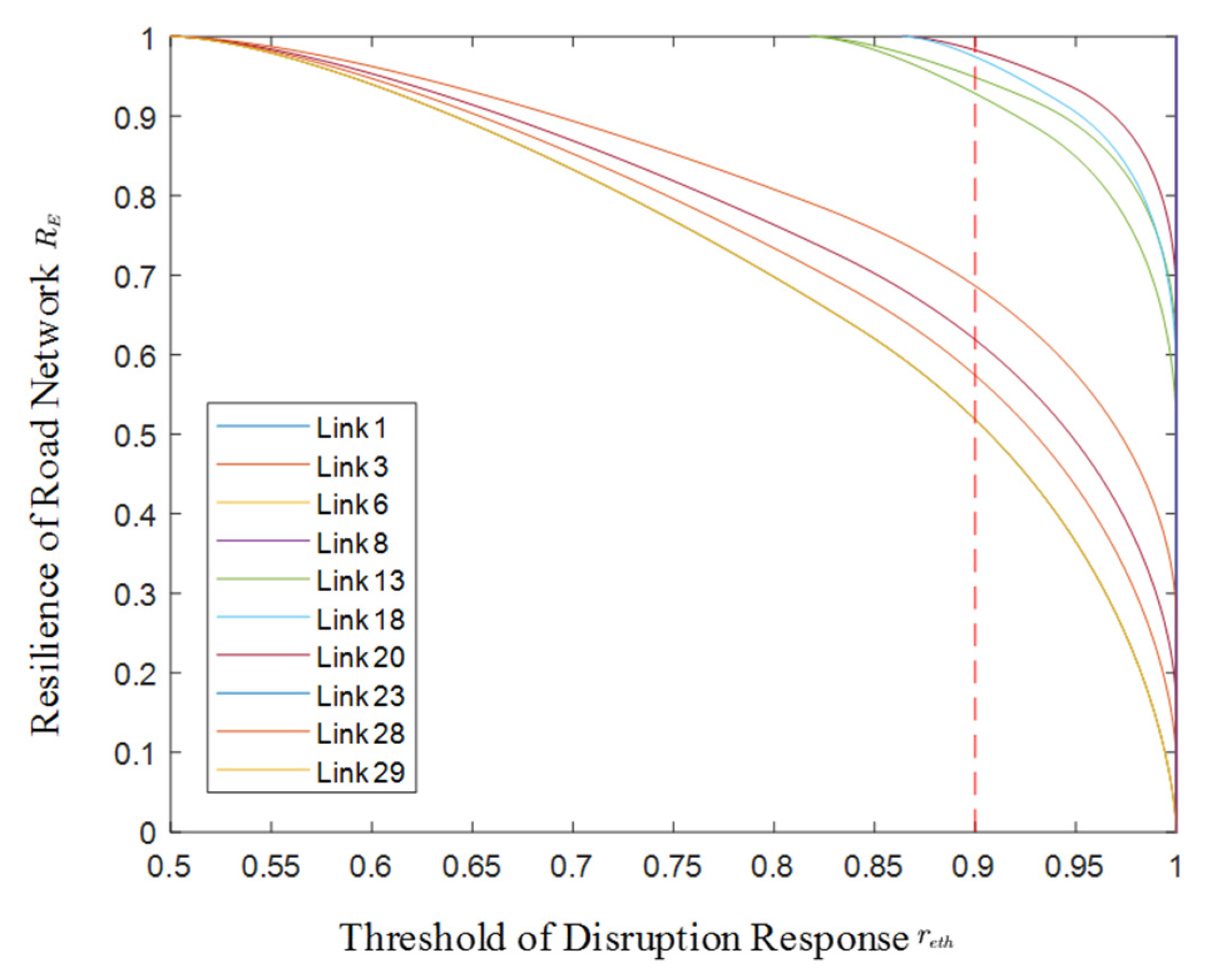
Resilience of the optimal network for different .


Table 1.
Parameter values in Figure 6.
Table 1.
Parameter values in Figure 6.
| 1 | 3 | 5 |
| 2 | 6 | 7 |
| 3 | 3 | 4 |
| 4 | 0 | 1 |
| 5 | 3 | 3 |
| 6 | 0 | 2 |
| 7 | 4 | 4 |
| 8 | 3 | 5 |
| 9 | 3 | 4 |
| 10 | 8 | 9 |
| 11 | 1 | 1 |
| 12 | 6 | 6 |
Table 2.
Resilience of system.
| Link | Resilience | Link | Resilience |
|---|---|---|---|
| 1 | 0.879 | 7 | 0.66 |
| 2 | 0.644 | 8 | 0.879 |
| 3 | 0.833 | 9 | 0.833 |
| 4 | 1 | 10 | 0.565 |
| 5 | 0.746 | 11 | 1 |
| 6 | 1 | 12 | 0.557 |
Table 3.
Parameters of optimization model and algorithm.
| Parameter | Value | |
|---|---|---|
| Optimization model | 0.9 | |
| 0.5 | ||
| Max-flow constraint | 20 | |
| Genetic algorithm | Population NIIND | 100 |
| Generation MAXGEN | 100 | |
| Generation gap GGAP | 0.4 | |
| Cross rate XOVR | 1 | |
| Mutation rate MUTR | 0.1 | |
Table 4.
Resilience of optimal network for different disruptions.
| Link | Resilience | Link | Resilience |
|---|---|---|---|
| 1 | 0.5184 | 18 | 0.9486 |
| 3 | 0.5184 | 20 | 0.9744 |
| 6 | 0.9281 | 23 | 0.6188 |
| 8 | 0.9827 | 28 | 0.6864 |
| 13 | 0.5741 | 29 | 0.5184 |
Publisher’s Note: MDPI stays neutral with regard to jurisdictional claims in published maps and institutional affiliations. |
© 2022 by the authors. Licensee MDPI, Basel, Switzerland. This article is an open access article distributed under the terms and conditions of the Creative Commons Attribution (CC BY) license (https://creativecommons.org/licenses/by/4.0/).
Share and Cite
MDPI and ACS Style
Dong, Q.; Li, R.; Kang, R. System Resilience Evaluation and Optimization Considering Epistemic Uncertainty. Symmetry 2022, 14, 1182. https://0-doi-org.brum.beds.ac.uk/10.3390/sym14061182
AMA Style
Dong Q, Li R, Kang R. System Resilience Evaluation and Optimization Considering Epistemic Uncertainty. Symmetry. 2022; 14(6):1182. https://0-doi-org.brum.beds.ac.uk/10.3390/sym14061182
Chicago/Turabian StyleDong, Qiang, Ruiying Li, and Rui Kang. 2022. "System Resilience Evaluation and Optimization Considering Epistemic Uncertainty" Symmetry 14, no. 6: 1182. https://0-doi-org.brum.beds.ac.uk/10.3390/sym14061182
Note that from the first issue of 2016, this journal uses article numbers instead of page numbers. See further details here.