Risk-Based Maintenance Optimization for a Subsea Production System with Epistemic Uncertainty

Abstract

The lack of operation and maintenance data brings difficulties to traditional risk assessment based on probability methods. Therefore, experts are invited to evaluate the key performance indicators related to system risk. These evaluation results are usually described by ambiguous language, so they have epistemic uncertainty. Uncertainty theory is a branch of mathematics used to model experts’ degrees of belief. The uncertain measure has duality, that is, some symmetry, which means that the sum of the uncertain measure of an event and the uncertain measure of its complementary set is equal to 1. Therefore, the risk occurrence time of each basic event evaluated by experts is modeled by the uncertain variable in this article. Then, the risk assessment method of systems with epistemic uncertainty is proposed based on an uncertain fault tree analysis. Furthermore, two risk-based maintenance optimization models for systems with epistemic uncertainty are established. In particular, the leakage risk assessment method and the two risk-based maintenance optimization models for a subsea production system are considered, and the optimization results are given. The optimization results can help practitioners to warn of the leakage risk and make scientific maintenance decisions based on expert knowledge, so as to extend the service life of subsea production systems.

1. Introduction

With the sustained and rapid development of the national economy, the demand for oil and gas resources all over the world is becoming more and more urgent. Marine oil and gas reserves are rich, which is of great significance in the energy strategy. Therefore, the exploration of marine oil and gas resources is also increasing. Submarine accidents have gradually increased with the rapid development of the offshore oil and gas industry, which can cause pipeline breaks, oil and gas leakage, serious environmental pollution, huge economic losses, and even casualties. As one of the most widely used production facilities operates in the submarine environment, it is necessary to make quantitative risk assessment and scientific maintenance decision-making for subsea production systems.

A fault tree (FT) is a tree-logic causality diagram, which uses event symbols and logic gate symbols to describe the causality between various events in the system. The “AND” gate implies that the output event will occur if all the input events occur, while the “OR” gate implies that the output event will occur if any one of the input events occur. Fault tree analysis (FTA) is a top–down deductive failure analysis for estimating the risk by using Boolean logic. FTA solves the occurrence probability of the top event according to the probability of occurrence of each basic event. In the past few decades, FTA has been successfully applied in many fields for risk assessment. For instance, Ruijters and Stoelinga [1] surveyed over 150 papers on FTA and provided an in-depth overview of the state-of-the-art in FTA. Sianipar and Adams [2] presented the use of a fault tree for the qualitative and quantitative evaluation of element-interaction phenomena. Volkanovski et al. [3] analyzed the reliability of a power system using a fault tree, in which the fault trees were related to the disruption of energy delivery from generators to the specific load points. Sun et al. [4] proposed a reliability-assessment method for a cyber-physical distribution network, in which the sequential fault processing and corresponding results considering the cyber impact were established based on the fault tree. Ikwan et al. [5] used a quantitative analysis of relevant risks through the development of fault-tree-analysis and risk-analysis methods to aid in real-time risk prediction and safety evaluation of leaks in a storage tank. Bhsttacharyya and Cheliyan [6] considered the optimization problem of a subsea production system for cost and reliability using its fault tree model. Based on the historical fault data of the spreaders accumulated during their online service for 13 years, Zheng et al. [7] built a complete spreader fault tree with three layers of fault phenomena, fault classification, and fault causes. Dickerson et al. [8] was concerned with developing a formal transformation method that mapped control flows modeled in unified modeling language activities to semantically equivalent fault trees. Ben El-Shanawany et al. [9] developed a closed-form approximation for the fault tree’s top event-uncertainty distribution, which was applicable when the uncertainties in the basic events of the model were log-normally distributed. Matsuoka [10] presented a procedure to solve mutually dependent fault trees in the expression of success events. Wang et al. [11] built a fault tree to analyze the causes of fire accidents and used the the Fussell Vesely importance method to compare the contribution degrees of the basic events.

In conventional FTA, the probabilities of failure of basic events are considered as exact values or random variables. However, the data are severely lacking in the field of subsea production systems, so it is unrealistic to evaluate the failure probabilities of basic events in its fault tree. Then, experts are invited to evaluate the degrees of belief about basic events. Cheliyan and Bhattacharyya [12] introduced fuzzy set theory to deal with subjective opinions of experts and calculated the failure probabilities of the intermediate events and the top event through the fault tree. Unfortunately, Liu [13] showed, via an example, that fuzzy theory was inappropriate to model the degree belief. A similar situation exists in the risk evaluation of subsea production systems. For example, the leakage risk of a subsea production system at time t is evaluated by expert as “approximately 0.01”. If the leakage risk of the subsea production system is regarded as a triangular fuzzy variable (0.05, 0.01, 0.15), it can be concluded that the possibility of “the leakage risk of the subsea production system is exactly 0.01” is 1, and the possibility of “the leakage risk of the subsea production system is not 0.01” is 1, based on the possibility measure. It is usually believed that the probability of “the leakage risk of the subsea production system is exactly 0.01” is 0. In addition, “the leakage risk of the subsea production system is exactly 0.01” and “the leakage risk of the subsea production system is not 0.01” have the same possibility value. This contradictory result also shows that the leakage risk evaluation of subsea production is unsuitable to be modeled by fuzzy theory, since the possibility measure does not have the duality property.

In order to measure the degree of belief, uncertainty theory was founded by Liu [14] and refined by Liu [15] based on normality, duality, subadditivity, and product-measure axioms. In recent years, uncertainty theory was widely used in various fields, such as structural reliability assessment [16], time series analysis [17], risk assessment [18], reliability modelling [19], and statistics [20].

In the past, several contributions have used various genetic algorithms as optimization techniques in the field of system reliability, in which the system was represented by a fault tree. Andrews and Bartlett [21] used GA for single-objective optimization of a firewater deluge system on an offshore platform, in which the system was presented by the structure of the fault tree. Pattison and Andrews [22] described a design optimization scheme for systems that required a high likelihood of functioning on demand by using GA. Bhsttacharyya and Cheliyan [6] solved a subsea production system optimization problem using GA and NSGA-II, in which the risk was evaluated by fault tree analysis. The difference between GA and NSGA-II, which are used in this paper, is that the fault tree analysis method adopts an uncertain algorithm.

The major contributions of this study are as follows: the risk occurrence time of each basic event evaluated by experts is modeled by an uncertain variable; the risk-assessment method of systems with epistemic uncertainty is proposed based on uncertain fault tree analysis; two risk-based maintenance optimization models for systems with epistemic uncertainty are established; the leakage risk assessment method and the two risk-based maintenance optimization models for a subsea production system are considered, and the optimization results are given.

The remainder of this article is organized as follows. Section 2 recalls some basic concepts related to uncertain variables. In Section 3, the risk assessment method of systems with epistemic uncertainty is proposed by using an uncertain fault tree analysis, and then two risk-based maintenance optimization models are established; in addition, the steps of GA and NSGA-II are given to solve the two optimization models. In Section 4, a leakage risk assessment and two risk-based maintenance optimization models for a subsea production system are considered, and then the optimization results are given.

2. Preliminaries

Let $\mathsf{\Gamma }$ be a nonempty set and Ł a $\sigma$-algebra over $\mathsf{\Gamma }$. Each element $\mathsf{\Lambda }\in \mathrm{Ł}$ is called an event. Then a number M$\left\{\mathsf{\Lambda }\right\}$ will be assigned to each event $\mathsf{\Lambda }$ to indicate the degree of belief with which we believe that $\mathsf{\Lambda }$ will happen. In order to rationally and scientifically describe a degree of belief, Liu [14] proposed the normality, duality, subadditivity, and product measure axioms.

Definition 1

(Liu [14]). The set function M is called an uncertain measure if it satisfies the normality, duality, subadditivity, and product measure axioms.

Definition 2

(Liu [14]). Let Γ be a nonempty set, Ł a σ-algebra over Γ, and M an uncertain measure. Then, the triplet $(\mathsf{\Gamma },\mathrm{Ł},M)$ is called an uncertainty space.

Definition 3

(Liu [14]). An uncertain variable is a function ξ from an uncertainty space $(\mathsf{\Gamma },\mathrm{Ł},M)$ to the set of real numbers such that $\{\mathsf{\xi }\in \mathcal{B}\}$ is an event for any Borel set $\mathcal{B}$ of real numbers.

Definition 4

(Liu [14]). The uncertainty distribution Φ of an uncertain variable ξ is defined by

$$\mathsf{\Phi }\left(x\right)=M\left\{\mathsf{\xi }\le x\right\}$$

for any real number x.

Definition 5

(Liu [15]). An uncertain variable ξ is called normal if it has a normal uncertainty distribution

$$\mathsf{\Phi }\left(x\right)={\left(1+exp\left(\frac{\pi (e-x)}{\sqrt{3}\sigma }\right)\right)}^{-1},x\in \mathcal{R},$$

denoted by $\mathcal{N}(e,\sigma )$, where e and σ are real numbers with $\sigma >0$.

Definition 6

(Liu [23]). The uncertain variables ${\mathsf{\xi }}_1,{\mathsf{\xi }}_2,\dots ,{\mathsf{\xi }}_n$ are said to be independent if

$$M\left\{\bigcap _{i=1}^n\{{\mathsf{\xi }}_i\in {\mathcal{B}}_i\}\right\}=\underset{i=1}{\overset{n}{\bigwedge }}M\{{\mathsf{\xi }}_i\in {\mathcal{B}}_i\}$$

(1)

for any Borel sets ${\mathcal{B}}_1,{\mathcal{B}}_2,\dots ,{\mathcal{B}}_n$ of real numbers. (⋀ is the minimum operator.)

Theorem 1

(Liu [23]). The uncertain variables ${\mathsf{\xi }}_1,{\mathsf{\xi }}_2,\dots ,{\mathsf{\xi }}_n$ are independent if and only if

$$M\left\{\bigcup _{i=1}^n\{{\mathsf{\xi }}_i\in {\mathcal{B}}_i\}\right\}=\underset{i=1}{\overset{n}{\bigvee }}M\{{\mathsf{\xi }}_i\in {\mathcal{B}}_i\}$$

(2)

for any Borel sets ${\mathcal{B}}_1,{\mathcal{B}}_2,\dots ,{\mathcal{B}}_n$ of real numbers. (⋁ is the maximum operator).

3. Risk-Based Maintenance Optimization Models for a System with Epistemic Uncertainty

The risk of systems with epistemic uncertainty is evaluated by an uncertain fault tree in this section. Then two risk-based maintenance optimization models based on uncertain fault tree are established, respectively.

3.1. System Risk Assessment

The risk of systems with epistemic uncertainty can be evaluated by uncertain fault tree. A fault tree is called an uncertain fault tree if the occurrence of all basic events is evaluated by an uncertain measure. Let ${\mathsf{\Lambda }}_1,{\mathsf{\Lambda }}_2,\dots ,{\mathsf{\Lambda }}_n$ be the independent input events. By Definition 6 and Theorem 1, the risk of the output event $\mathsf{\Lambda }$, i.e., the belief degree of occurrence of the output event $\mathsf{\Lambda }$, is

$$M\left\{\mathsf{\Lambda }\right\}=\left\{\begin{array}{c}{\displaystyle \underset{i=1}{\overset{n}{\bigwedge }}M\left\{{\mathsf{\Lambda }}_i\right\},\mathrm{for} “\mathrm{AND}” \mathrm{gate}}\hfill \\ {\displaystyle \underset{i=1}{\overset{n}{\bigvee }}M\left\{{\mathsf{\Lambda }}_i\right\},\mathrm{for} “\mathrm{OR}” \mathrm{gate}.}\hfill \end{array}\right.$$

(3)

Let $T_1,T_2,\dots ,T_n$ be the failure occurrence times of independent input events ${\mathsf{\Lambda }}_1,{\mathsf{\Lambda }}_2,\dots ,$${\mathsf{\Lambda }}_n$, respectively. Suppose that $T_1,T_2,\dots ,T_n$ are uncertain variables with uncertain distributions ${\mathsf{\Phi }}_1\left(t\right),$${\mathsf{\Phi }}_2\left(t\right),\dots ,{\mathsf{\Phi }}_n\left(t\right)$. Denote the state of the input event ${\mathsf{\Lambda }}_i$ at time t by ${\mathsf{\xi }}_i\left(t\right)$, $i=1,2,\dots ,n$. Let ${\mathsf{\xi }}_i\left(t\right)=1$ if ${\mathsf{\Lambda }}_i$ occurs at time t and ${\mathsf{\xi }}_i\left(t\right)=0$ if ${\mathsf{\Lambda }}_i$ does not occur at time t. It is easy to see that ${\mathsf{\xi }}_i\left(t\right)$, $i=1,2,\dots ,n$ are uncertain variables and

$${\mathsf{\xi }}_i\left(t\right)=\left\{\begin{array}{cc}\hfill & 1,\mathrm{with}\mathrm{uncertain}\mathrm{measure}{\mathsf{\Phi }}_i\left(t\right)\hfill \\ \hfill & 0,\mathrm{with}\mathrm{uncertain}\mathrm{measure}1-{\mathsf{\Phi }}_i\left(t\right).\hfill \end{array}\right.$$

(4)

Then, the risk of input event ${\mathsf{\Lambda }}_i$ at time t is the belief degree of uncertain event “$\{{\mathsf{\xi }}_i\left(t\right)=1\}$”, which is just ${\mathsf{\Phi }}_i\left(t\right)$, $i=1,2,\dots ,n$.

Denote the state of the output event $\mathsf{\Lambda }$ at time t by $\mathsf{\xi }\left(t\right)$. Let $\mathsf{\xi }\left(t\right)=1$ if $\mathsf{\Lambda }$ occurs at time t. If ${\mathsf{\Lambda }}_1,{\mathsf{\Lambda }}_2,\dots ,{\mathsf{\Lambda }}_n$ are connected by the “AND” gate, then the risk of the output event $\mathsf{\Lambda }$ at time t is

$$\begin{array}{cc}\mathsf{\Phi }\left(t\right)\hfill & {\displaystyle =M\left\{\mathsf{\xi }\right(t)=1\}}\hfill \\ & {\displaystyle =M\left\{\bigcap _{i=1}^n\{{\mathsf{\xi }}_i\left(t\right)=1\}\right\}}\hfill \\ & {\displaystyle =\underset{i=1}{\overset{n}{\bigwedge }}M\{{\mathsf{\xi }}_i\left(t\right)=1\}=\underset{i=1}{\overset{n}{\bigwedge }}{\mathsf{\Phi }}_i\left(t\right).}\hfill \end{array}$$

If ${\mathsf{\Lambda }}_1,{\mathsf{\Lambda }}_2,\dots ,{\mathsf{\Lambda }}_n$ are connected by the “OR” gate, then the risk of the output event $\mathsf{\Lambda }$ at time t is

$$\begin{array}{cc}\mathsf{\Phi }\left(t\right)\hfill & {\displaystyle =M\left\{\mathsf{\xi }\right(t)=1\}}\hfill \\ & {\displaystyle =M\left\{\bigcup _{i=1}^n\{{\mathsf{\xi }}_i\left(t\right)=1\}\right\}}\hfill \\ & {\displaystyle =\underset{i=1}{\overset{n}{\bigvee }}M\left\{{\mathsf{\xi }}_i\left(t\right)=1\right\}=\underset{i=1}{\overset{n}{\bigvee }}{\mathsf{\Phi }}_i\left(t\right).}\hfill \end{array}$$

Then the risk of the output event $\mathsf{\Lambda }$ at time t can be summarized as follows

$$\mathsf{\Phi }\left(t\right)=\left\{\begin{array}{c}{\displaystyle \underset{i=1}{\overset{n}{\bigwedge }}{\mathsf{\Phi }}_i\left(t\right),\mathrm{for} “\mathrm{AND}” \mathrm{gate}}\hfill \\ {\displaystyle \underset{i=1}{\overset{n}{\bigvee }}{\mathsf{\Phi }}_i\left(t\right),\mathrm{for} “\mathrm{OR}” \mathrm{gate}.}\hfill \end{array}\right.$$

(5)

If the occurrence times of all basic events and their uncertain distributions are given, Equation (5) can be extended to any fault tree structure to evaluate the system risk at time t. Then the following theorem is proposed.

Theorem 2.

Let ${\mathsf{\Phi }}_1\left(x\right),{\mathsf{\Phi }}_2\left(x\right),\dots ,{\mathsf{\Phi }}_n\left(x\right)$ be distribution functions of occurrence times of basic events ${\mathsf{\Lambda }}_1,{\mathsf{\Lambda }}_2,\dots ,{\mathsf{\Lambda }}_n$, respectively, and let $T^U$ be the uncertain fault tree structure function of the system consisting of ⋀ and ⋁ operators. Then, the system risk at time t is

$${\mathsf{\Phi }}_{Top}\left(t\right)=T^U({\mathsf{\Phi }}_1\left(t\right),{\mathsf{\Phi }}_2\left(t\right),\dots ,{\mathsf{\Phi }}_n\left(t\right)).$$

(6)

3.2. Maintenance Cost

Consider an uncertain fault tree that consists of N independent basic events, where n basic events have cost functions, since there are more than one choices of maintenance technologies for these events, denoted by ${\mathsf{\Lambda }}_i,i=1,2,\dots ,n$. The maintenance cost of basic event ${\mathsf{\Lambda }}_i$ at time t (denoted by $C_i\left(t\right)$) is related with its maintenance measures at time t. The maintenance measures of basic event ${\mathsf{\Lambda }}_i$ at time t can be transformed to the degree of risk aversion, denoted by $M_i\left(t\right)$, $i=1,2,\dots ,n$. Then the maintenance cost of basic event ${\mathsf{\Lambda }}_i$ at time t is

$$C_i\left(t\right)=F_i\left(M_i\left(t\right)\right),$$

(7)

where $F_i$ is called the “risk-cost” function. Usually, $F_i$ is non-increasing with respect to $M_i\left(t\right),i=1,2,\dots ,n$.

It is assumed that if the system is maintained, all basic events are repaired and incomplete maintenance is usually adopted. Therefore, the total maintenance cost at time t is

$$\begin{array}{cc}{C}_{Top}\left(t\right)\hfill & {\displaystyle =\sum _{i=1}^n{C}_i\left(t\right)=\sum _{i=1}^n{F}_i\left(M_i\left(t\right)\right).}\hfill \end{array}$$

(8)

3.3. Risk-Based Maintenance Optimization Models

3.3.1. The Single-Objective Maintenance Optimization Model

The aim of the single-objective optimization model is to determine the maintenance strategy $M_1\left(t\right),M_2\left(t\right),\dots ,M_n\left(t\right)$ at any time t when the total maintenance cost is minimized under the risk constraints. Denote the system risk at time t by ${\mathsf{\Phi }}_{Top}\left(t\right)$. It is easy to see that ${\mathsf{\Phi }}_{Top}\left(t\right)$ is the function of $M_1\left(t\right),M_2\left(t\right),\dots ,M_n\left(t\right)$. Then, the single-objective maintenance optimization model is established by

$$\left\{\begin{array}{c}\mathrm{Min}{C}_{Top}\left(t\right)\hfill \\ s.t.\hfill \\ {\mathsf{\Phi }}_{Top}\left(t\right)\le \tau \left(t\right)\hfill \\ 0\le M_i\left(t\right)\le {\mathsf{\Phi }}_i\left(t\right),i=1,2,\dots ,n,\hfill \end{array}\right.$$

(9)

where ${\mathsf{\Phi }}_{Top}\left(t\right)$ is calculated by Equation (6), $C_{Top}\left(t\right)$ is calculated by Equation (8), and $\tau \left(t\right)$ is the given allowable risk level of the system at time t. Since the uncertain fault tree structure function $T^U$ is monotonic non-decreasing, the range of $\tau \left(t\right)$ is usually in $0\le \tau \left(t\right)\le T^U({\mathsf{\Phi }}_1\left(t\right),\dots ,{\mathsf{\Phi }}_n\left(t\right)).$

3.3.2. The Multi-Objective Maintenance Optimization Model

The aim of the multi-objective optimization model is to determine the maintenance strategy $M_1\left(t\right),M_2\left(t\right),\dots ,M_n\left(t\right)$ at any time t to minimize the system risk and the total maintenance cost at the same time. The multi-objective optimization model is established by

$$\left\{\begin{array}{c}\mathrm{Min}{C}_{Top}\left(t\right)\hfill \\ \mathrm{Min}{\mathsf{\Phi }}_{Top}\left(t\right)\hfill \\ s.t.\hfill \\ 0\le M_i\left(t\right)\le {\mathsf{\Phi }}_i\left(t\right),i=1,2,\dots ,n,\hfill \end{array}\right.$$

(10)

where ${\mathsf{\Phi }}_{Top}\left(t\right)$ and $C_{Top}\left(t\right)$ can be calculated by Equations (6) and (8), respectively.

3.4. Solutions of the Optimization Problems

The solution to the single-objective maintenance optimization model (9) can be obtained by GA. Compared with some conventional optimization algorithms, GA can usually obtain better optimization results faster. The solution to the multi-objective maintenance optimization model (10) can be obtained by NSGA-II, since it reduces the complexity of the non-inferior sorting genetic algorithm and has the advantages of fast running speed and good convergence of the solution set.

3.4.1. The Genetic Algorithm

Step 1: Initialization

For basic events ${\mathsf{\Lambda }}_i,i=1,2,\dots ,n$, the maintenance strategies are generated by

$$M_i\left(t\right)={\alpha }_i\times {\mathsf{\Phi }}_i\left(t\right),i=1,2,\dots ,n,$$

(11)

where ${\alpha }_i,i=1,2,\dots ,n$ are random numbers generated in interval [0,1] and generated with each iteration. $M_i\left(t\right),i=1,2,\dots ,n$ constitute a chromosome structure. $(M_1\left(t\right),M_2\left(t\right),\dots ,M_n\left(t\right))$ constitute a chromosome structure. $M_i\left(t\right),i=1,2,\dots ,n$, ${\mathsf{\Phi }}_i\left(t\right),$$i=1,2,\dots ,n,$, and the fault tree structure are used to calculate the system risk ${\mathsf{\Phi }}_{Top}\left(t\right)$. If ${\mathsf{\Phi }}_{top}\left(t\right)\le \tau \left(t\right)$, a chromosome is generated. Predetermined the allowable risk level of the system at time t, denoted by $\tau \left(t\right)$. If ${\mathsf{\Phi }}_{top}\left(t\right)>\tau \left(t\right)$, chromosomes need to be regenerated by Equation (11). Repeat the above process until k chromosomes are generated. The maintenance strategy of basic event ${\mathsf{\Lambda }}_i$ in the jth chromosome is denoted as $M_i^{\left(j\right)}\left(t\right),i=1,2,\dots ,n,j=1,2,\dots ,k$.

Step 2: Selection

Consider $\frac{1}{C_{Top}\left(t\right)}$ as the fitness function.The roulette algorithm is used for selection.

Step 3: Crossover

Select individuals $M_i^{\left(j_1\right)}\left(t\right)$ and $M_i^{\left(j_2\right)}\left(t\right)$, $0\le j_1,j_2\le k,j_1\ne j_2$ randomly in the current population to generate new individuals by

$$M_i^{\left(j_1^{\prime }\right)}\left(t\right)=0.5[(1+r_1)\times M_i^{\left(j_1\right)}\left(t\right)+(1-r_1)\times M_i^{\left(j_2\right)}\left(t\right)]$$

(12)

and

$$M_i^{\left(j_2^{\prime }\right)}\left(t\right)=0.5[(1-r_1)\times M_i^{\left(j_1\right)}\left(t\right)+(1+r_1)\times M_i^{\left(j_2\right)}\left(t\right)],$$

(13)

in which

$$r_1=\left\{\begin{array}{cc}{\left(2u_1\right)}^{\frac{1}{\eta +1}},\hfill & \mathrm{if}{u}_1\le 0.5\hfill \\ {\left[\frac{1}{2(1-u_1)}\right]}^{\frac{1}{\eta +1}},\hfill & \mathrm{if}{u}_1>0.5,\hfill \end{array}\right.$$

where $u_1$ is a random number in [0, 1] and $\eta >0$ is a distribution index.

Step 4: Mutation

The individuals participating in mutation are selected randomly with probability p, and the new individuals after mutation are generated by the following formula

$$M_i^{\left(j^{\prime }\right)}\left(t\right)=M_i^{\left(j\right)}\left(t\right)-\delta ·{\mathsf{\Phi }}_i\left(t\right)$$

(14)

in which

$$\delta =\left\{\begin{array}{cc}{[2u_2+(1-2u_2)\times {(1-{\delta }_1)}^{{\eta }_m+1}]}^{\frac{1}{{\eta }_m+1}}-1,\hfill & \mathrm{if}{u}_2\le 0.5\hfill \\ 1-{[2(1-u_2)+2(u_2-0.5)\times {(1-{\delta }_2)}^{{\eta }_m+1}]}^{\frac{1}{{\eta }_m+1}},\hfill & \mathrm{if}{u}_2>0.5,\hfill \end{array}\right.$$

where $u_2$ is the random number in the interval [0,1], ${\eta }_m$ is the distribution index, and ${\delta }_1$ and ${\delta }_2$ are generated by

$${\delta }_1=\frac{M_i^{\left(j\right)}\left(t\right)-{\mathsf{\Phi }}_i\left(t\right)}{0-{\mathsf{\Phi }}_i\left(t\right)}\mathrm{and}{\delta }_2=\frac{0-M_i^{\left(j\right)}\left(t\right)}{0-{\mathsf{\Phi }}_i\left(t\right)},$$

respectively. Then, continue step 2 until the end of step 4. The chromosome constructs a near-optimal solution.

3.4.2. The Non-Dominated Sorting Genetic Algorithm II

Step 1: Initialization

For each basic event ${\mathsf{\Lambda }}_i$, the maintenance strategy is generated by

$$M_i\left(t\right)={\alpha }_i\times {\mathsf{\Phi }}_i\left(t\right)$$

where ${\alpha }_i$ is a random number generated in interval [0, 1] and generated with each iteration. $M_i\left(t\right),i=1,2,\dots ,n$ constitute a chromosome structure. Suppose that the initial population consists of k chromosomes, denoted by $X^{\left(j\right)},j=1,2,\dots ,k$. The maintenance strategy of the basic event ${\mathsf{\Lambda }}_i$ in the jth chromosome is denoted as $M_i^{\left(j\right)}\left(t\right),i=1,2,\dots ,n,j=1,2,\dots ,k$.

Step 2: Fast non-dominated sort

Calculate the objective functions ${\mathsf{\Phi }}_{Top}^{\left(j\right)}\left(t\right)$ and $C_{Top}^{\left(j\right)}\left(t\right),j=1,2,\dots ,k$, respectively. Arrange these chromosomes by using the fast non-dominated sorting approach in Deb et al. [24] and arrive the set $X_1^{\left(j\right)},j=1,2,\dots ,k$.

Step 3: Crossover

Select individuals $M_i^{\left(j_1\right)}\left(t\right)$ and $M_i^{\left(j_2\right)}\left(t\right)$, $0\le j_1,j_2\le k,j_1\ne j_2$ randomly to generate new individuals by

$$M_i^{\left(j_1^{\prime }\right)}\left(t\right)=0.5[(1+r_2)\times M_i^{\left(j_1\right)}\left(t\right)+(1-r_2)\times M_i^{\left(j_2\right)}\left(t\right)]$$

and

$$M_i^{\left(j_2^{\prime }\right)}\left(t\right)=0.5[(1-r_2)\times M_i^{\left(j_1\right)}\left(t\right)+(1+r_2)\times M_i^{\left(j_2\right)}\left(t\right)],$$

in which

$$r_2=\left\{\begin{array}{cc}{\left(2u_3\right)}^{\frac{1}{\eta +1}},\hfill & \mathrm{if}{u}_3\le 0.5\hfill \\ {\left[\frac{1}{2(1-u_3)}\right]}^{\frac{1}{\eta +1}},\hfill & \mathrm{if}{u}_3>0.5,\hfill \end{array}\right.$$

where $u_3$ is a random number in [0,1] and $\eta >0$ is a distribution index.

Step 4: Mutation

The individuals that undergo the mutation are selected randomly with probability p, and the new individuals after the mutation are generated by

$$M_i^{\left(j^{\prime }\right)}\left(t\right)=M_i^{\left(j\right)}\left(t\right)-{\delta }_3·{\mathsf{\Phi }}_i\left(t\right),$$

in which

$${\delta }_3=\left\{\begin{array}{cc}{[2u_4+(1-2u_4)\times {(1-{\delta }_4)}^{{\eta }_m+1}]}^{\frac{1}{{\eta }_m+1}}-1,\hfill & \mathrm{if}{u}_4\le 0.5\hfill \\ 1-{[2(1-u_4)+2(u_4-0.5)\times {(1-{\delta }_5)}^{{\eta }_m+1}]}^{\frac{1}{{\eta }_m+1}},\hfill & \mathrm{if}{u}_4>0.5,\hfill \end{array}\right.$$

where $u_4$ is a random number in the interval [0,1], ${\eta }_m$ is the distribution index, ${\delta }_4$ and ${\delta }_5$ are generated by

$${\delta }_4=\frac{M_i^{\left(j\right)}\left(t\right)-{\mathsf{\Phi }}_i\left(t\right)}{0-{\mathsf{\Phi }}_i\left(t\right)}and{\delta }_5=\frac{0-M_i^{\left(j\right)}\left(t\right)}{0-{\mathsf{\Phi }}_i\left(t\right)},$$

respectively. Then, k new chromosomes are generated, denoted by ${\left(X^{\left(j\right)}\right)}^{{}^{\prime }},j=1,2,\dots ,k$.

Step 5: Elite retention strategy

Combine $X_1^{\left(j\right)},j=1,2,\dots ,k$ and ${\left(X^{\left(j\right)}\right)}^{{}^{\prime }},j=1,2,\dots ,k$ together to construct a $2k$ chromosome set, denoted by ${\left(X_1^{\left(j\right)}\right)}^{{}^{″}},j=1,2,\dots ,2k$. Compute the objective functions ${\left({\mathsf{\Phi }}_{Top}^{\left(j\right)}\left(t\right)\right)}^{{}^{\prime }}$ and ${\left(C_{Top}^{\left(j\right)}\left(t\right)\right)}^{{}^{\prime }}$ by ${\left(X_1^{\left(j\right)}\right)}^{{}^{\prime }},j=1,2,\dots ,k$. Rearrange the chromosome set ${\left(X_1^j\right)}^{{}^{″}},j=1,2,\dots ,2k$ and retain the top k chromosomes as the chromosome set $X_2^{\left(j\right)},j=1,2,\dots ,k$. Rename $X_2^{\left(j\right)}$ by $X_1^{\left(j\right)},j=1,2,\dots ,k$ and go to step 3 until the end of step 5. The chromosomes construct near-optimal Pareto front.

4. Risk-Based Maintenance Optimization Models for a Subsea Production System

Subsea production systems are the main lifeline of offshore oil and gas exploitation and consist of Xmas-trees, manifolds, jumper tube, umbilical cable, pipelines, etc. In this section, the fault tree structure of the subsea production system in Cheliyan and Bhattacharyya [12] is still used. However, the traditional fault tree analysis is replaced by the uncertain fault tree analysis and is extended to a time-varying situation, which can be used to evaluate the risk of the subsea production system at any time. Then, two risk-based maintenance optimization models for the subsea production system are given. In addition, GA and NSGA-II are used to solve the two optimization models. The result can help practitioners to give early warning of oil and gas leakage risk and make scientific maintenance decisions.

4.1. The Leakage Risk Assessment for the Subsea Production System

Consider a subsea production system in an extremely harsh marine environment. The fault tree of the subsea production system takes “oil and gas leakage” as the top event (denoted by ${\mathsf{\Lambda }}_{Top}$) and consists of 40 events (denoted by ${\mathsf{\Lambda }}_i,i=1,2,\dots ,40$), in which ${\mathsf{\Lambda }}_i,i=1,\dots ,26$ are basic events and ${\mathsf{\Lambda }}_i,i=27,\dots ,40$ are intermediate events. Let $T_i,i=1,2,\dots ,40$ be the uncertain failure occurrence times of events ${\mathsf{\Lambda }}_i,i=1,2,\dots ,40$, respectively. Suppose that $T_i,i=1,2,\dots ,26$ are evaluated by domain experts. The detailed descriptions of the top event, intermediate events, and basic events are shown in

Table 1. Information of the top event and intermediate events.

Events	Descriptions	Gates	Connected Events
${\mathsf{\Lambda }}_{Top}$	Oil and gas leakage	OR	${\mathsf{\Lambda }}_{26},{\mathsf{\Lambda }}_{38},{\mathsf{\Lambda }}_{39},{\mathsf{\Lambda }}_{40}$
${\mathsf{\Lambda }}_{40}$	Leakage in key facilities	OR	${\mathsf{\Lambda }}_{32},{\mathsf{\Lambda }}_{33},{\mathsf{\Lambda }}_{34},{\mathsf{\Lambda }}_{35},{\mathsf{\Lambda }}_{37}$
${\mathsf{\Lambda }}_{39}$	Leakage in pipe	AND	${\mathsf{\Lambda }}_{11},{\mathsf{\Lambda }}_{36}$
${\mathsf{\Lambda }}_{38}$	Leakage in gas or oil well	AND	${\mathsf{\Lambda }}_1,{\mathsf{\Lambda }}_2$
${\mathsf{\Lambda }}_{37}$	Connector leakage	AND	${\mathsf{\Lambda }}_{17},{\mathsf{\Lambda }}_{31}$
${\mathsf{\Lambda }}_{36}$	Defect in pipe	OR	${\mathsf{\Lambda }}_{27},{\mathsf{\Lambda }}_{28},{\mathsf{\Lambda }}_{29},{\mathsf{\Lambda }}_{30}$
${\mathsf{\Lambda }}_{35}$	PLEM leakage	AND	${\mathsf{\Lambda }}_{24},{\mathsf{\Lambda }}_{25}$
${\mathsf{\Lambda }}_{34}$	PLET leakage	AND	${\mathsf{\Lambda }}_{22},{\mathsf{\Lambda }}_{23}$
${\mathsf{\Lambda }}_{33}$	Manifold leakage	AND	${\mathsf{\Lambda }}_{20},{\mathsf{\Lambda }}_{21}$
${\mathsf{\Lambda }}_{32}$	X-tree leakage	AND	${\mathsf{\Lambda }}_{18},{\mathsf{\Lambda }}_{19}$
${\mathsf{\Lambda }}_{31}$	Defect in connector	OR	${\mathsf{\Lambda }}_{12},{\mathsf{\Lambda }}_{13},{\mathsf{\Lambda }}_{14},{\mathsf{\Lambda }}_{15},{\mathsf{\Lambda }}_{16}$
${\mathsf{\Lambda }}_{30}$	Defect in riser	OR	${\mathsf{\Lambda }}_9,{\mathsf{\Lambda }}_{10}$
${\mathsf{\Lambda }}_{29}$	Defect in pipeline	OR	${\mathsf{\Lambda }}_7,{\mathsf{\Lambda }}_8$
${\mathsf{\Lambda }}_{28}$	Defect in flowline	OR	${\mathsf{\Lambda }}_5,{\mathsf{\Lambda }}_6$
${\mathsf{\Lambda }}_{27}$	Defect in jumper	OR	${\mathsf{\Lambda }}_3,{\mathsf{\Lambda }}_4$

and

Table 2. Information of basic events.

Basic Events	Descriptions	Failure Occurrence Times	Failure Time Distributions
${\mathsf{\Lambda }}_1$	Overpressure in well	$T_1$	$\mathcal{N}(10,3)$
${\mathsf{\Lambda }}_2$	Failure of control in well	$T_2$	$\mathcal{N}(11,3)$
${\mathsf{\Lambda }}_3$	Jumper puncture	$T_3$	$\mathcal{N}(12,3.5)$
${\mathsf{\Lambda }}_4$	Jumper rupture	$T_4$	$\mathcal{N}(10,2.5)$
${\mathsf{\Lambda }}_5$	Flowline puncture	$T_5$	$\mathcal{N}(8,2.4)$
${\mathsf{\Lambda }}_6$	Flowline rupture	$T_6$	$\mathcal{N}(8,2.5)$
${\mathsf{\Lambda }}_7$	Pipeline puncture	$T_7$	$\mathcal{N}(11,3)$
${\mathsf{\Lambda }}_8$	Pipeline rupture	$T_8$	$\mathcal{N}(11,2.8)$
${\mathsf{\Lambda }}_9$	Riser puncture	$T_9$	$\mathcal{N}(10,3)$
${\mathsf{\Lambda }}_{10}$	Riser rupture	$T_{10}$	$\mathcal{N}(9,2.5)$
${\mathsf{\Lambda }}_{11}$	Failure of leakage control of pipe	$T_{11}$	$\mathcal{N}(9,3)$
${\mathsf{\Lambda }}_{12}$	Defect in X-tree wellhead connector	$T_{12}$	$\mathcal{N}(8,2.4)$
${\mathsf{\Lambda }}_{13}$	Defect in pipe connector	$T_{13}$	$\mathcal{N}(9,3)$
${\mathsf{\Lambda }}_{14}$	Defect in pipe manifold connector	$T_{14}$	$\mathcal{N}(10,3.5)$
${\mathsf{\Lambda }}_{15}$	Defect in pipe-PLET connector	$T_{15}$	$\mathcal{N}(10,3.2)$
${\mathsf{\Lambda }}_{16}$	Defect in pipe-PLEM connector	$T_{16}$	$\mathcal{N}(11,3.2)$
${\mathsf{\Lambda }}_{17}$	Failure of connector leakage control	$T_{17}$	$\mathcal{N}(11,2.9)$
${\mathsf{\Lambda }}_{18}$	Defect in X-tree	$T_{18}$	$\mathcal{N}(9,3)$
${\mathsf{\Lambda }}_{19}$	Failure of X-tree leakage control	$T_{19}$	$\mathcal{N}(9,3)$
${\mathsf{\Lambda }}_{20}$	Defect in manifold	$T_{20}$	$\mathcal{N}(8,2.6)$
${\mathsf{\Lambda }}_{21}$	Failure of manifold leakage control	$T_{21}$	$\mathcal{N}(10,3.2)$
${\mathsf{\Lambda }}_{22}$	Defect in PLET	$T_{22}$	$\mathcal{N}(11,3)$
${\mathsf{\Lambda }}_{23}$	Failure of PLET leakage control	$T_{23}$	$\mathcal{N}(9,3)$
${\mathsf{\Lambda }}_{24}$	Defect in PLEM	$T_{24}$	$\mathcal{N}(10,3)$
${\mathsf{\Lambda }}_{25}$	Failure of PLEM leakage control	$T_{25}$	$\mathcal{N}(8,3)$
${\mathsf{\Lambda }}_{26}$	Third party damage	$T_{26}$	$\mathcal{N}(10,2.6)$

.

Denote the uncertainty distributions of the failure occurrence time of the top event by ${\mathsf{\Phi }}_{Top}\left(t\right)$, and denote the uncertainty distribution of $T_i$ by ${\mathsf{\Phi }}_i\left(t\right),i=1,2,\dots ,40$. By Theorem 2, we can arrive at

$$\begin{array}{cc}{\mathsf{\Phi }}_{Top}\left(t\right)\hfill & {\displaystyle ={\mathsf{\Phi }}_{26}\left(t\right)\vee {\mathsf{\Phi }}_{38}\left(t\right)\vee {\mathsf{\Phi }}_{39}\left(t\right)\vee {\mathsf{\Phi }}_{40}\left(t\right)}\hfill \\ \hfill & {\displaystyle ={\mathsf{\Phi }}_{26}\left(t\right)\vee \left({\mathsf{\Phi }}_1\left(t\right)\wedge {\mathsf{\Phi }}_2\left(t\right)\right)\vee \left({\mathsf{\Phi }}_{11}\left(t\right)\wedge {\mathsf{\Phi }}_{36}\left(t\right)\right)}\hfill \\ \hfill & {\displaystyle \vee \left({\mathsf{\Phi }}_{32}\left(t\right)\vee {\mathsf{\Phi }}_{33}\left(t\right)\vee {\mathsf{\Phi }}_{34}\left(t\right)\vee {\mathsf{\Phi }}_{35}\left(t\right)\vee {\mathsf{\Phi }}_{37}\left(t\right)\right)}\hfill \\ \hfill & {\displaystyle =\left({\mathsf{\Phi }}_1\left(t\right)\wedge {\mathsf{\Phi }}_2\left(t\right)\right)\vee {\mathsf{\Phi }}_{26}\left(t\right)\vee \left({\mathsf{\Phi }}_{11}\left(t\right)\wedge \left({\mathsf{\Phi }}_{27}\left(t\right)\vee {\mathsf{\Phi }}_{28}\left(t\right)\vee {\mathsf{\Phi }}_{29}\left(t\right)\vee {\mathsf{\Phi }}_{30}\left(t\right)\right)\right)}\hfill \\ \hfill & {\displaystyle \vee \left({\mathsf{\Phi }}_{18}\left(t\right)\wedge {\mathsf{\Phi }}_{19}\left(t\right)\right)\vee \left({\mathsf{\Phi }}_{20}\left(t\right)\wedge {\mathsf{\Phi }}_{21}\left(t\right)\right)\vee \left({\mathsf{\Phi }}_{22}\left(t\right)\wedge {\mathsf{\Phi }}_{23}\left(t\right)\right)}\hfill \\ \hfill & {\displaystyle \vee \left({\mathsf{\Phi }}_{24}\left(t\right)\wedge {\mathsf{\Phi }}_{25}\left(t\right)\right)\vee \left({\mathsf{\Phi }}_{17}\left(t\right)\wedge {\mathsf{\Phi }}_{31}\left(t\right)\right)}\hfill \\ \hfill & {\displaystyle =\left({\mathsf{\Phi }}_1\left(t\right)\wedge {\mathsf{\Phi }}_2\left(t\right)\right)\vee \left({\mathsf{\Phi }}_{18}\left(t\right)\wedge {\mathsf{\Phi }}_{19}\left(t\right)\right)}\hfill \\ \hfill & {\displaystyle \vee \left({\mathsf{\Phi }}_{11}\left(t\right)\wedge \left(\left({\mathsf{\Phi }}_3\left(t\right)\vee {\mathsf{\Phi }}_4\left(t\right)\right)\vee \left({\mathsf{\Phi }}_5\left(t\right)\vee {\mathsf{\Phi }}_6\left(t\right)\right)\right.\right.}\hfill \\ \hfill & {\displaystyle \left.\left.\vee \left({\mathsf{\Phi }}_7\left(t\right)\vee {\mathsf{\Phi }}_8\left(t\right)\right)\vee \left({\mathsf{\Phi }}_9\left(t\right)\vee {\mathsf{\Phi }}_{10}\left(t\right)\right)\right)\right)}\hfill \\ \hfill & {\displaystyle \vee \left({\mathsf{\Phi }}_{20}\left(t\right)\wedge {\mathsf{\Phi }}_{21}\left(t\right)\right)\vee \left({\mathsf{\Phi }}_{22}\left(t\right)\wedge {\mathsf{\Phi }}_{23}\left(t\right)\right)\vee \left({\mathsf{\Phi }}_{24}\left(t\right)\wedge {\mathsf{\Phi }}_{25}\left(t\right)\right)}\hfill \\ \hfill & {\displaystyle \vee {\mathsf{\Phi }}_{26}\left(t\right)\vee \left({\mathsf{\Phi }}_{17}\left(t\right)\wedge \left({\mathsf{\Phi }}_{12}\left(t\right)\vee {\mathsf{\Phi }}_{13}\left(t\right)\vee {\mathsf{\Phi }}_{14}\left(t\right)\vee {\mathsf{\Phi }}_{15}\left(t\right)\vee {\mathsf{\Phi }}_{16}\left(t\right)\left)\right)\right.\right.}\hfill \end{array}.$$

(15)

Bring the data in Table 1 into Formula (15) to obtain the specific distribution function. As shown in Figure 1, when the subsea production system is put into use in the early stage, the leakage risk is relatively low. As the service period grows, the leakage risk of the subsea production system increases gradually. This conclusion can assist decision makers in quantitatively assessing the risk status of the subsea production system at any time, so as to make early warnings and take corresponding maintenance measures.

4.2. The Maintenance Cost for the Subsea Production System

Suppose that basic events ${\mathsf{\Lambda }}_i,i=1,2\dots ,25$ have cost functions, since there are more than one choices of maintenance technologies for these events. The risk-cost functions $F_i,i=1,2,\dots ,25$ are considered linear functions, which means that they can be determined by the slopes in

Table 3. The slopes for risk-cost functions (Unit: million dollars).

Basic events	${\mathit{\Lambda }}_1$	${\mathit{\Lambda }}_2$	${\mathit{\Lambda }}_3$	${\mathit{\Lambda }}_4$	${\mathit{\Lambda }}_5$
Slopes	${\displaystyle \frac{2000}{43}}$	${\displaystyle \frac{5000}{83}}$	${\displaystyle \frac{300}{19}}$	${\displaystyle \frac{750}{47}}$	${\displaystyle \frac{2500}{7}}$
Basic events	${\mathsf{\Lambda }}_6$	${\mathsf{\Lambda }}_7$	${\mathsf{\Lambda }}_8$	${\mathsf{\Lambda }}_9$	${\mathsf{\Lambda }}_{10}$
Slopes	${\displaystyle \frac{5000}{19}}$	${\displaystyle \frac{10,000}{13}}$	${\displaystyle \frac{60,000}{103}}$	${\displaystyle \frac{3500}{23}}$	${\displaystyle \frac{4375}{36}}$
Basic events	${\mathsf{\Lambda }}_{11}$	${\mathsf{\Lambda }}_{12}$	${\mathsf{\Lambda }}_{13}$	${\mathsf{\Lambda }}_{14}$	${\mathsf{\Lambda }}_{15}$
Slopes	${\displaystyle \frac{5000}{269}}$	${\displaystyle \frac{500}{13}}$	${\displaystyle \frac{1500}{41}}$	${\displaystyle \frac{15,000}{193}}$	${\displaystyle \frac{800}{7}}$
Basic events	${\mathsf{\Lambda }}_{16}$	${\mathsf{\Lambda }}_{17}$	${\mathsf{\Lambda }}_{18}$	${\mathsf{\Lambda }}_{19}$	${\mathsf{\Lambda }}_{20}$
Slopes	${\displaystyle \frac{10,000}{183}}$	${\displaystyle \frac{625}{113}}$	${\displaystyle \frac{20,000}{199}}$	${\displaystyle \frac{125}{2}}$	${\displaystyle \frac{5000}{17}}$
Basic events	${\mathsf{\Lambda }}_{21}$	${\mathsf{\Lambda }}_{22}$	${\mathsf{\Lambda }}_{23}$	${\mathsf{\Lambda }}_{24}$	${\mathsf{\Lambda }}_{25}$
Slopes	${\displaystyle \frac{15,000}{223}}$	${\displaystyle \frac{20,000}{189}}$	${\displaystyle \frac{3750}{107}}$	${\displaystyle \frac{20,000}{189}}$	${\displaystyle \frac{7500}{107}}$

.

Take the risk-cost function of ${\mathsf{\Lambda }}_{15}$, for example, its “risk-cost” function is shown in Figure 2.

4.3. Risk-Based Maintenance Optimization Models for the Subsea Production System

4.3.1. The Single-Objective Maintenance Optimization Model

The single-objective optimization model described in (9) is considered. The risks of basic events avoided after taking maintenance measures at time t are considered as decision variables, denoted by $M_i\left(t\right),i=1,2,\dots ,25$. Then the single-objective optimization model for the subsea production system can be expressed by

$$\left\{\begin{array}{c}\mathrm{Min}{C}_{Top}\left(t\right)\hfill \\ s.t.\hfill \\ {\mathsf{\Phi }}_{Top}\left(t\right)\le \tau \left(t\right)\hfill \\ 0\le M_i\left(t\right)\le {\mathsf{\Phi }}_i\left(t\right),i=1,2,\dots ,25,\hfill \end{array}\right.$$

(16)

in which

$$\begin{array}{cc}{\mathsf{\Phi }}_{Top}\left(t\right)\hfill & {\displaystyle =T^U({\mathsf{\Phi }}_1\left(t\right)-M_1\left(t\right),\dots ,{\mathsf{\Phi }}_{26}\left(t\right)-M_{26}\left(t\right))}\hfill \\ \hfill & {\displaystyle =\left(({\mathsf{\Phi }}_1\left(t\right)-M_1\left(t\right))\wedge ({\mathsf{\Phi }}_2\left(t\right)-M_2\left(t\right))\right)\vee \left(({\mathsf{\Phi }}_{18}\left(t\right)-M_{18}\left(t\right))\wedge ({\mathsf{\Phi }}_{19}\left(t\right)-M_{19}\left(t\right))\right)}\hfill \\ \hfill & {\displaystyle \vee \left(({\mathsf{\Phi }}_{11}\left(t\right)-M_{11}\left(t\right))\wedge \left(\left(({\mathsf{\Phi }}_3\left(t\right)-M_3\left(t\right))\vee ({\mathsf{\Phi }}_4\left(t\right)-M_4\left(t\right))\right)\right.\right.}\hfill \\ \hfill & {\displaystyle \vee \left(({\mathsf{\Phi }}_5\left(t\right)-M_5\left(t\right))\vee ({\mathsf{\Phi }}_6\left(t\right)-M_6\left(t\right))\right)\vee \left(({\mathsf{\Phi }}_7\left(t\right)-M_7\left(t\right))\vee ({\mathsf{\Phi }}_8\left(t\right)-M_8\left(t\right))\right)}\hfill \\ \hfill & {\displaystyle \left.\left.\vee \left(({\mathsf{\Phi }}_9\left(t\right)-M_9\left(t\right))\vee ({\mathsf{\Phi }}_{10}\left(t\right)-M_{10}\left(t\right))\right)\right)\right)}\hfill \\ \hfill & {\displaystyle \vee \left(({\mathsf{\Phi }}_{20}\left(t\right)-M_{20}\left(t\right))\wedge ({\mathsf{\Phi }}_{21}\left(t\right)-M_{21}\left(t\right))\right)\vee \left(({\mathsf{\Phi }}_{22}\left(t\right)-M_{22}\left(t\right))\wedge ({\mathsf{\Phi }}_{23}\left(t\right)-M_{23}\left(t\right))\right)}\hfill \\ \hfill & {\displaystyle \vee \left(({\mathsf{\Phi }}_{24}\left(t\right)-M_{24}\left(t\right))\wedge ({\mathsf{\Phi }}_{25}\left(t\right)-M_{25}\left(t\right))\right)\vee {\mathsf{\Phi }}_{26}\left(t\right)}\hfill \\ \hfill & {\displaystyle \vee \left(({\mathsf{\Phi }}_{17}\left(t\right)-M_{17}\left(t\right))\wedge \left(({\mathsf{\Phi }}_{12}\left(t\right)-M_{12}\left(t\right))\vee ({\mathsf{\Phi }}_{13}\left(t\right)-M_{13}\left(t\right))\right.\right.}\hfill \\ \hfill & {\displaystyle \left.\vee (({\mathsf{\Phi }}_{14}\left(t\right)-M_{14}\left(t\right))\vee ({\mathsf{\Phi }}_{15}\left(t\right)-M_{15}\left(t\right))\vee ({\mathsf{\Phi }}_{16}\left(t\right)-M_{16}\left(t\right))\right)}\hfill \end{array}$$

(17)

and

$$\begin{array}{cc}{C}_{Top}\left(t\right)\hfill & {\displaystyle =\sum _{i=1}^{25}{F}_i\left(M_i\left(t\right)\right)}\hfill \\ \hfill & {\displaystyle =\frac{2000}{43}{M}_1\left(t\right)+\frac{5000}{83}{M}_2\left(t\right)+\frac{300}{19}{M}_3\left(t\right)+\frac{750}{47}{M}_4\left(t\right)+\frac{2500}{7}{M}_5\left(t\right)}\hfill \\ \hfill & {\displaystyle \frac{5000}{19}{M}_6\left(t\right)+\frac{10,000}{13}{M}_7\left(t\right)+\frac{60,000}{103}{M}_8\left(t\right)+\frac{3500}{23}{M}_9\left(t\right)+\frac{4375}{36}{M}_{10}\left(t\right)}\hfill \\ \hfill & {\displaystyle \frac{5000}{269}{M}_{11}\left(t\right)+\frac{500}{13}{M}_{12}\left(t\right)+\frac{1500}{41}{M}_{13}\left(t\right)+\frac{15,000}{193}{M}_{14}\left(t\right)+\frac{800}{7}{M}_{15}\left(t\right)}\hfill \\ \hfill & {\displaystyle \frac{10,000}{183}{M}_{16}\left(t\right)+\frac{625}{113}{M}_{17}\left(t\right)+\frac{20,000}{199}{M}_{18}\left(t\right)+\frac{125}{2}{M}_{19}\left(t\right)+\frac{5000}{17}{M}_{20}\left(t\right)}\hfill \\ \hfill & {\displaystyle \frac{15,000}{223}{M}_{21}\left(t\right)+\frac{20,000}{189}{M}_{22}\left(t\right)+\frac{3750}{107}{M}_{23}\left(t\right)+\frac{20,000}{189}{M}_{24}\left(t\right)+\frac{7500}{107}{M}_{25}\left(t\right).}\hfill \end{array}$$

(18)

Remark 1.

The objective function $C_{Top}\left(t\right)$ does not include the maintenance cost of ${\mathsf{\Lambda }}_{26}$ since it does not involve multiple maintenance technologies, so it does not participate in the optimization process.

The single-objective optimization model can be solved by the GA. The key parameters of the GA are assigned as follows: $\tau \left(t\right)$ is set from 0 to $T^U({\mathsf{\Phi }}_1\left(t\right),\dots ,{\mathsf{\Phi }}_{26}\left(t\right))$, the population size is 100, the crossover probability is 0.8, the mutation probability is 0.04, and the number of generations is 100. The relationship between maintenance time t, ${\mathsf{\Phi }}_{Top}\left(t\right)$, and Min $C_{Top}\left(t\right)$ are presented in Figure 3, in which “×” denotes the optimized solutions in the eighth year. In particular, if $\tau \left(t\right)$ is set to $T^U(0.7{\mathsf{\Phi }}_1\left(8\right),\dots ,0.7{\mathsf{\Phi }}_{26}\left(8\right))$, the optimal maintenance strategy $M_i^{*}\left(8\right),i=1,2,\dots ,25$ can refer to

Table 4. The optimal maintenance strategy in the eighth year.

${\mathit{M}}_1^{*}\left(8\right)$	${\mathit{M}}_2^{*}\left(8\right)$	${\mathit{M}}_3^{*}\left(8\right)$	${\mathit{M}}_4^{*}\left(8\right)$	${\mathit{M}}_5^{*}\left(8\right)$	${\mathit{M}}_6^{*}\left(8\right)$	${\mathit{M}}_7^{*}\left(8\right)$	${\mathit{M}}_8^{*}\left(8\right)$	${\mathit{M}}_9^{*}\left(8\right)$
$0.0329$	$0.0124$	$0.0045$	$0.0427$	$0.1500$	$0.1500$	$0.0068$	$0.0124$	$0.0288$
$M_{10}^{*}\left(8\right)$	$M_{11}^{*}\left(8\right)$	$M_{12}^{*}\left(8\right)$	$M_{13}^{*}\left(8\right)$	$M_{14}^{*}\left(8\right)$	$M_{15}^{*}\left(8\right)$	$M_{16}^{*}\left(8\right)$	$M_{17}^{*}\left(8\right)$	$M_{18}^{*}\left(8\right)$
$0.0779$	$0.0665$	$0.1500$	$0.0638$	$0.0329$	$0.0427$	$0.0150$	$0.0150$	$0.0759$
$M_{19}^{*}\left(8\right)$	$M_{20}^{*}\left(8\right)$	$M_{21}^{*}\left(8\right)$	$M_{22}^{*}\left(8\right)$	$M_{23}^{*}\left(8\right)$	$M_{24}^{*}\left(8\right)$	$M_{25}^{*}\left(8\right)$
$0.0779$	$0.1500$	$0.0246$	$0.0150$	$0.0779$	$0.0329$	$0.1500$

and the optimal maintenance cost in the eighth year is $216.64$ million dollar. Then the leakage risk of the subsea production system after maintenance is shown in Figure 4.

This conclusion can give the solution to when and how much maintenance funds the enterprise needs to prepare under the allowable risk level, and then give the maintenance strategy for each basic event, so as to improve the enterprise’s risk- and maintenance-management abilities and extend the service life of the subsea production system.

Remark 2.

Take the situation of the subsea production system in the eighth year as an example. The relationship between the number of generations and Min $C_{Top}\left(8\right)$ is shown in Figure 5. It is easy to see that with the increase in the number of generations, the value of Min $C_{Top}\left(8\right)$ converges gradually. When the number of generations reaches 80, the value of Min $C_{Top}\left(8\right)$ has stabilized. Then, the number of generations in GA is set to 100.

4.3.2. The Multi-Objective Maintenance Optimization Model

The leakage risk of the subsea production system at time t can also be evaluated by uncertain failure tree analysis directly. Then, the muti-objective optimization model of the subsea production system can be established by (10), namely,

$$\left\{\begin{array}{c}\mathrm{Min}{C}_{Top}\left(t\right)\hfill \\ \mathrm{Min}{\mathsf{\Phi }}_{Top}\left(t\right)\hfill \\ s.t.\hfill \\ 0\le M_i\left(t\right)\le {\mathsf{\Phi }}_i\left(t\right),i=1,2,\dots ,25,\hfill \end{array}\right.$$

(19)

in which ${\mathsf{\Phi }}_{Top}\left(t\right)$ and $C_{Top}\left(t\right)$ are determined by Equations (17) and (18), respectively.

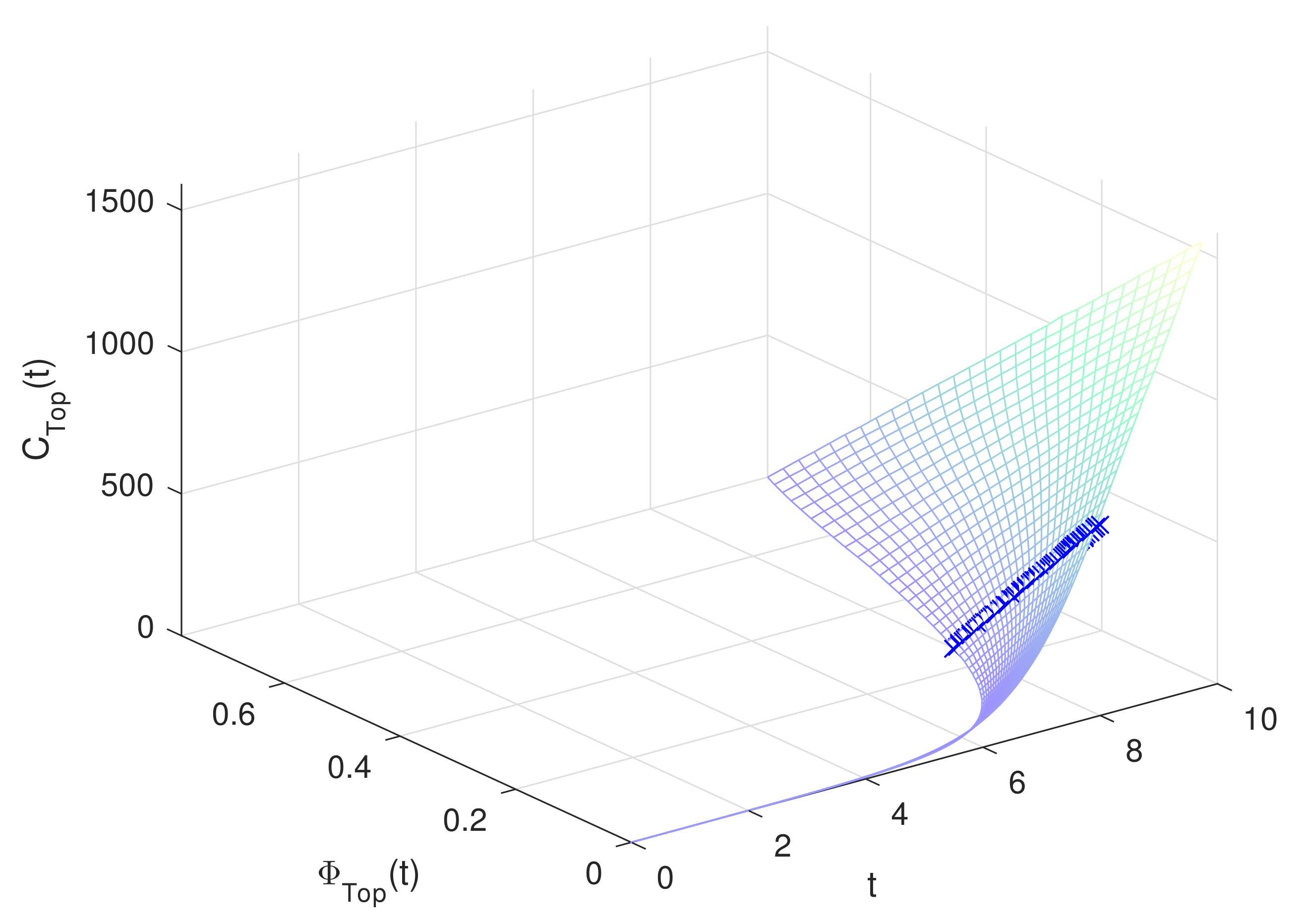
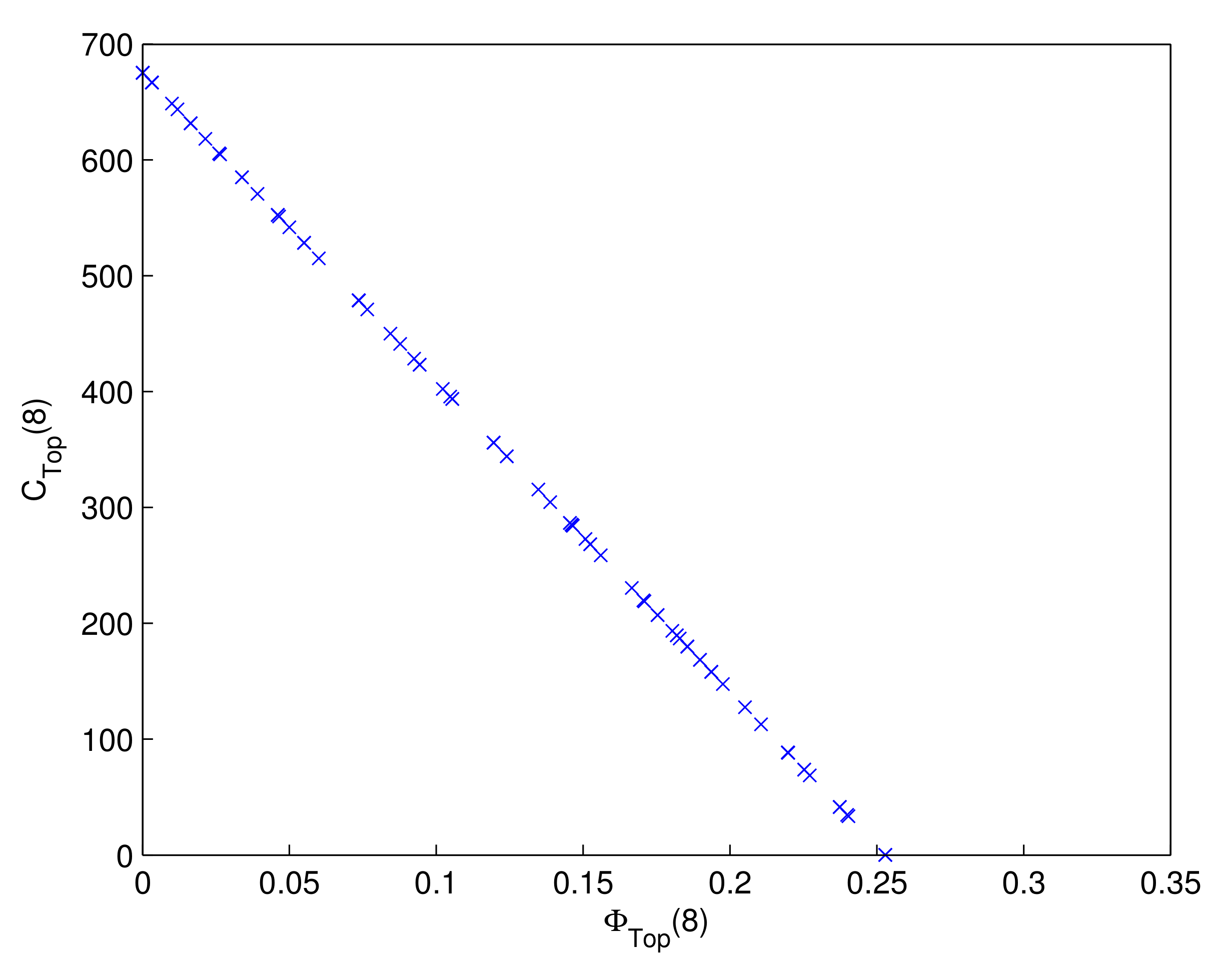
The multi-objective optimization model can be solved by NSGA-II. The key parameters of the NSGA-II are assigned as follows: the population size is 100, the crossover probability is 0.5, the mutation probability is 0.01, and the number of generations is 120. In Figure 6, the relationship between maintenance time t, ${\mathsf{\Phi }}_{Top}\left(t\right)$ and $C_{Top}\left(t\right)$ is presented, in which “×” denotes the optimized non-dominated solution set in the eighth year. In order to show the optimized non-dominated solution set of the eighth year more clearly, Figure 7 is given. In particular, when the point $(0.1359,312.13)$ in Figure 7 is selected, one of the optimal maintenance strategies is shown in

Table 5. One of the optimal maintenance strategies in the eighth year.

${\mathit{M}}_1^{*}\left(8\right)$	${\mathit{M}}_2^{*}\left(8\right)$	${\mathit{M}}_3^{*}\left(8\right)$	${\mathit{M}}_4^{*}\left(8\right)$	${\mathit{M}}_5^{*}\left(8\right)$	${\mathit{M}}_6^{*}\left(8\right)$	${\mathit{M}}_7^{*}\left(8\right)$	${\mathit{M}}_8^{*}\left(8\right)$	${\mathit{M}}_9^{*}\left(8\right)$
$0.0507$	$0.0191$	$0.0069$	$0.0658$	$0.2311$	$0.2311$	$0.0104$	$0.0191$	$0.0443$
$M_{10}^{*}\left(8\right)$	$M_{11}^{*}\left(8\right)$	$M_{12}^{*}\left(8\right)$	$M_{13}^{*}\left(8\right)$	$M_{14}^{*}\left(8\right)$	$M_{15}^{*}\left(8\right)$	$M_{16}^{*}\left(8\right)$	$M_{17}^{*}\left(8\right)$	$M_{18}^{*}\left(8\right)$
$0.1201$	$0.1024$	$0.2311$	$0.0983$	$0.0507$	$0.0658$	$0.0231$	$0.0231$	$0.1169$
$M_{19}^{*}\left(8\right)$	$M_{20}^{*}\left(8\right)$	$M_{21}^{*}\left(8\right)$	$M_{22}^{*}\left(8\right)$	$M_{23}^{*}\left(8\right)$	$M_{24}^{*}\left(8\right)$	$M_{25}^{*}\left(8\right)$
$0.1201$	$0.2311$	$0.0379$	$0.0231$	$0.1201$	$0.0507$	$0.2311$

.

This conclusion presents the relationship between the leakage risk and the total maintenance cost of the subsea production system at any time. It can help decision makers to arrange maintenance tasks according to the annual maintenance funds and give the maintenance strategy of each basic event.

Remark 3.

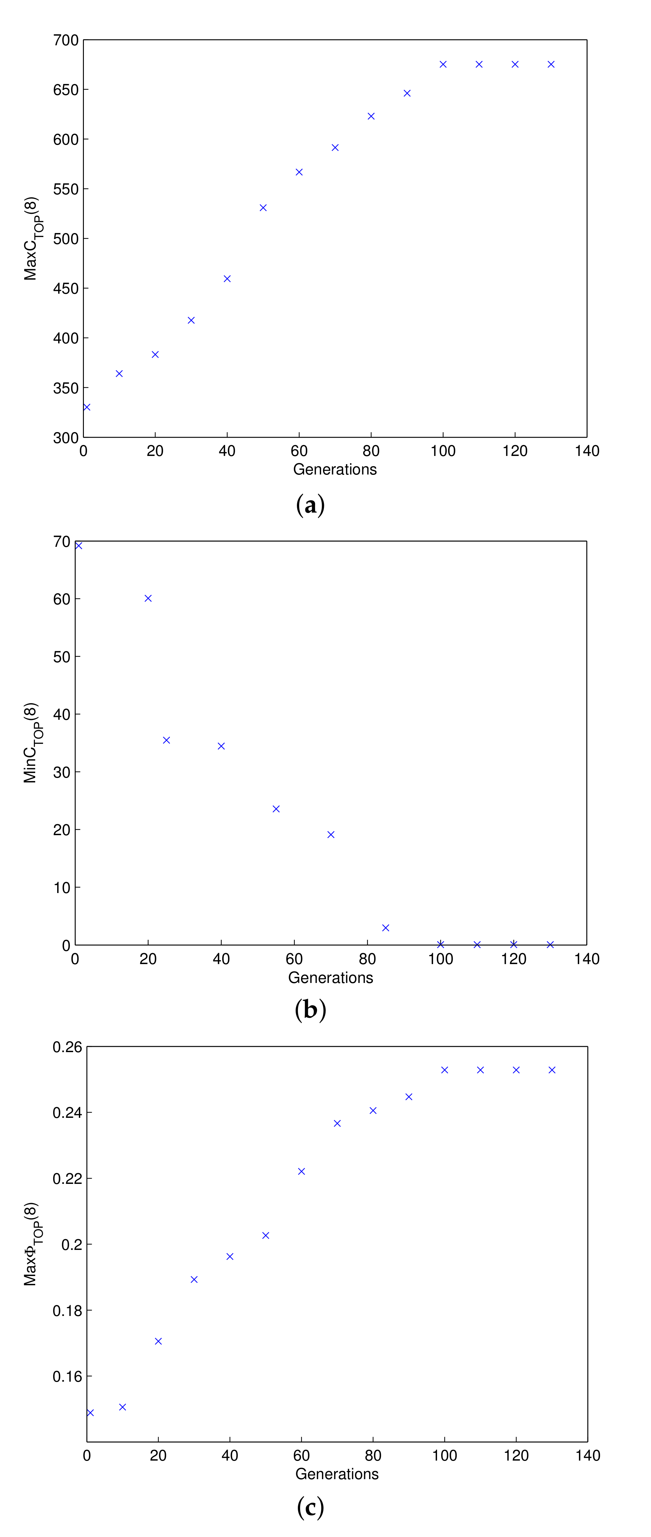
Take the situation of the subsea production system in the eighth year as an example. The ranges of $C_{Top}\left(8\right)$ and ${\mathsf{\Phi }}_{Top}\left(8\right)$ with the growth of generations is shown in Figure 8. It is easy to see that with the increase in the number of generations, the values of Max $C_{Top}\left(8\right)$, Min $C_{Top}\left(8\right)$, and Max ${\mathsf{\Phi }}_{Top}\left(8\right)$ converge gradually. When the number of generations reaches 100, the values of Max $C_{Top}\left(8\right)$, Min $C_{Top}\left(8\right)$, and Max ${\mathsf{\Phi }}_{Top}\left(8\right)$ have stabilized. The minimum value of Min ${\mathsf{\Phi }}_{Top}\left(8\right)$ is always around 0.067. Therefore, the number of generations in NSGA-II is set to 120.

5. Conclusions

The subsea production system is in a harsh submarine environment, which causes great difficulties in data acquisition and brings difficulties to the traditional risk-assessment methods. Experts are invited to evaluate the key performance indicators related to system risk, which are often described by ambiguous language. In this article, a risk-assessment method and two basic risk-based maintenance optimization models are established for systems with epistemic uncertainty, which are used in the field of a subsea production system. The specific contributions of this article are as follows:

(1)

The risk occurrence time of each basic event evaluated by experts is modeled by uncertain variable.

(2)

A risk assessment method for systems with epistemic uncertainty is proposed based on uncertain fault tree analysis.

(3)

Two risk-based maintenance optimization models for systems with epistemic uncertainty are established, and the specific calculation steps of the algorithms are presented accordingly.

(4)

The leakage risk of a subsea production system is given. On that basis, two risk-based optimization models for a subsea production system are established. In addition, the optimization results are given.

The current work can help practitioners to warn the leakage risk and make scientific maintenance decisions with only expert knowledge, so as to extend the service life of the subsea production system. In the future, the risk assessment method and risk-based maintenance optimization models will be applied to other equipment that are difficult to obtain sufficient data.

References

- Ruijters, E.; Stoelinga, M. Fault tree analysis: A survey of the state-of-the-art in modeling, analysis and tools. Comput. Sci. Rev. 2015, 15, 29–62. [Google Scholar] [CrossRef]
- Sianipar, P.R.M.; Adams, T.M. Fault-tree model of bridge element deterioration due to interaction. J. Infrastruct. Syst. 1997, 3, 103–110. [Google Scholar] [CrossRef]
- Volkanovski, A.; Čepin, M.; Mavko, B. Application of the fault tree analysis for assessment of power system reliability. Reliab. Eng. Syst. Saf. 2009, 94, 1116–1127. [Google Scholar] [CrossRef]
- Sun, X.; Liu, Y.L.; Deng, L.C. Reliability assessment of cyber-physical distribution network based on the fault tree. Renew. Energy 2020, 155, 1411–1424. [Google Scholar] [CrossRef]
- Ikwan, F.; Sanders, D.; Hassan, M. Safety evaluation of leak in a storage tank using fault tree analysis and risk matrix analysis. J. Loss Prev. Process Ind. 2021, 73, 104597. [Google Scholar] [CrossRef]
- Bhattacharyya, S.K.; Cheliyan, A.S. Optimization of a subsea production system for cost and reliability using its fault tree model. Reliab. Eng. Syst. Saf. 2019, 185, 213–219. [Google Scholar] [CrossRef]
- Zheng, Y.; Zhao, F.; Wang, Z. Fault diagnosis system of bridge crane equipment based on fault tree and bayesian network. Int. J. Adv. Manuf. Technol. 2019, 105, 3605–3618. [Google Scholar] [CrossRef]
- Dickerson, C.E.; Roslan, R.; Ji, S. A formal transformation method for automated fault tree generation from a UML activity model. IEEE Trans. Reliab. 2018, 67, 1219–1236. [Google Scholar] [CrossRef]
- El-Shanawany, A.B.; Ardron, K.H.; Walker, S.P. Lognormal approximations of fault tree uncertainty distributions. Risk Anal. 2018, 38, 1576–1584. [Google Scholar] [CrossRef]
- Matsuoka, T. Procedure to solve mutually dependent fault trees (FT with loops). Reliab. Eng. Syst. Saf. 2021, 214, 107667. [Google Scholar] [CrossRef]
- Wang, Y.F.; Liu, Z.M.; Jiang, J.C.; Khan, F.; Wang, J. Blowout fire probability prediction of offshore drilling platform based on system dynamics. J. Loss Prev. Process Ind. 2019, 62, 103960. [Google Scholar] [CrossRef]
- Cheliyan, A.S.; Bhattacharyya, S.K. Fuzzy fault tree analysis of oil and gas leakage in subsea production systems. J. Ocean Eng. Sci. 2018, 3, 38–48. [Google Scholar] [CrossRef]
- Liu, B.D. Why is there a need for uncertainty theory. J. Uncertain Syst. 2012, 6, 3–10. [Google Scholar]
- Liu, B.D. Uncertainty Theory, 2nd ed.; Springer: Berlin/Heidelberg, Germany, 2007. [Google Scholar]
- Liu, B.D. Uncertainty Theory: A Branch of Mathematics for Modeling Human Uncertainty; Springer: Berlin/Heidelberg, Germany, 2010. [Google Scholar]
- Liu, Y.; Zhao, J.Y.; Qu, Z.G.; Wang, L. Structural reliability assessment based on subjective uncertainty. Int. J. Comput. Methods 2021, 18, 2150046. [Google Scholar] [CrossRef]
- Ye, T.; Yang, X. Analysis and prediction of confirmed COVID-19 cases in china with uncertain time series. Fuzzy Optim. Decis. Mak. 2021, 20, 209C228. [Google Scholar] [CrossRef]
- Hu, L.H.; Kang, R.; Pan, X.; Zuo, D.J. Risk assessment of uncertain random system—Level-1 and level-2 joint propagation of uncertainty and probability in fault tree analysis. Reliab. Eng. Syst. Saf. 2020, 198, 106874. [Google Scholar] [CrossRef]
- Liu, Y.; Qu, Z.G.; Li, X.Z.; An, Y.; Yin, W.L. Reliability modeling for repairable systems with stochastic lifetimes and uncertain repair times. IEEE Trans. Fuzzy Syst. 2019, 27, 2396–2405. [Google Scholar] [CrossRef]
- Zu, T.; Kang, R.; Wen, M. Graduation formula: A new method to construct belief reliability distribution under epistemic uncertainty. J. Syst. Eng. Electron. 2020, 31, 626–633. [Google Scholar]
- Bartlett, J.A.a.L. Genetic algorithm optimization of a firewater deluge system. Qual. Reliab. Eng. Int. 2003, 19, 39–52. [Google Scholar]
- Pattison, R.; Andrews, J. Genetic algorithms in optimal safety system design. Proc. Inst. Mech. Eng. Part E J. Process Mech. Eng. 1999, 213, 187–197. [Google Scholar] [CrossRef]
- Liu, B.D. Some research problems in uncertainty theory. J. Uncertain Syst. 2009, 3, 3–10. [Google Scholar]
- Deb, K.; Pratap, A.; Agarwal, S.; Meyarivan, T. A fast and elitist multiobjective genetic algorithm: NSGA-II. IEEE Trans. Evol. Comput. 2002, 6, 182–197. [Google Scholar] [CrossRef]
Figure 1.
The uncertainty distribution of the failure occurrence time of the top event .
Figure 2.
The risk-cost function of .
Figure 3.
The relationship between maintenance time t, and Min .