One-Dimensional Convolutional Auto-Encoder for Predicting Furnace Blowback Events from Multivariate Time Series Process Data—A Case Study

Abstract

Modern industrial mining and mineral processing applications are characterized by large volumes of historical process data. Hazardous events occurring in these processes compromise process safety and therefore overall viability. These events are recorded in historical data and are often preceded by characteristic patterns. Reconstruction-based data-driven models are trained to reconstruct the characteristic patterns of hazardous event-preceding process data with minimal residuals, facilitating effective event prediction based on reconstruction residuals. This investigation evaluated one-dimensional convolutional auto-encoders as reconstruction-based data-driven models for predicting positive pressure events in industrial furnaces. A simple furnace model was used to generate dynamic multivariate process data with simulated positive pressure events to use as a case study. A one-dimensional convolutional auto-encoder was trained as a reconstruction-based model to recognize the data preceding the hazardous events, and its performance was evaluated by comparing it to a fully-connected auto-encoder as well as a principal component analysis reconstruction model. This investigation found that one-dimensional convolutional auto-encoders recognized event-preceding patterns with lower detection delays, higher specificities, and lower missed alarm rates, suggesting that the one-dimensional convolutional auto-encoder layout is superior to the fully connected auto-encoder layout for use as a reconstruction-based event prediction model. This investigation also found that the nonlinear auto-encoder models outperformed the linear principal component model investigated. While the one-dimensional auto-encoder was evaluated comparatively on a simulated furnace case study, the methodology used in this evaluation can be applied to industrial furnaces and other mineral processing applications. Further investigation using industrial data will allow for a view of the convolutional auto-encoder’s absolute performance as a reconstruction-based hazardous event prediction model.

1. Introduction

South Africa hosts the majority of the world’s platinum group metal (PGM)-reserves in the Bushveld Igneous Complex [1]. These PGMs are extracted from nickel-copper ores contained in the Bushveld Complex through a series of process steps. Mined ore undergoes comminution, liberating sulphides to create a sulphide concentrate that is concentrated through flotation. Flotation concentrates are smelted and converted, yielding a copper-nickel matte rich in PGMs. Precious metals within the matte are separated from base metals through hydrometallurgical treatments before being refined into their pure forms [2].

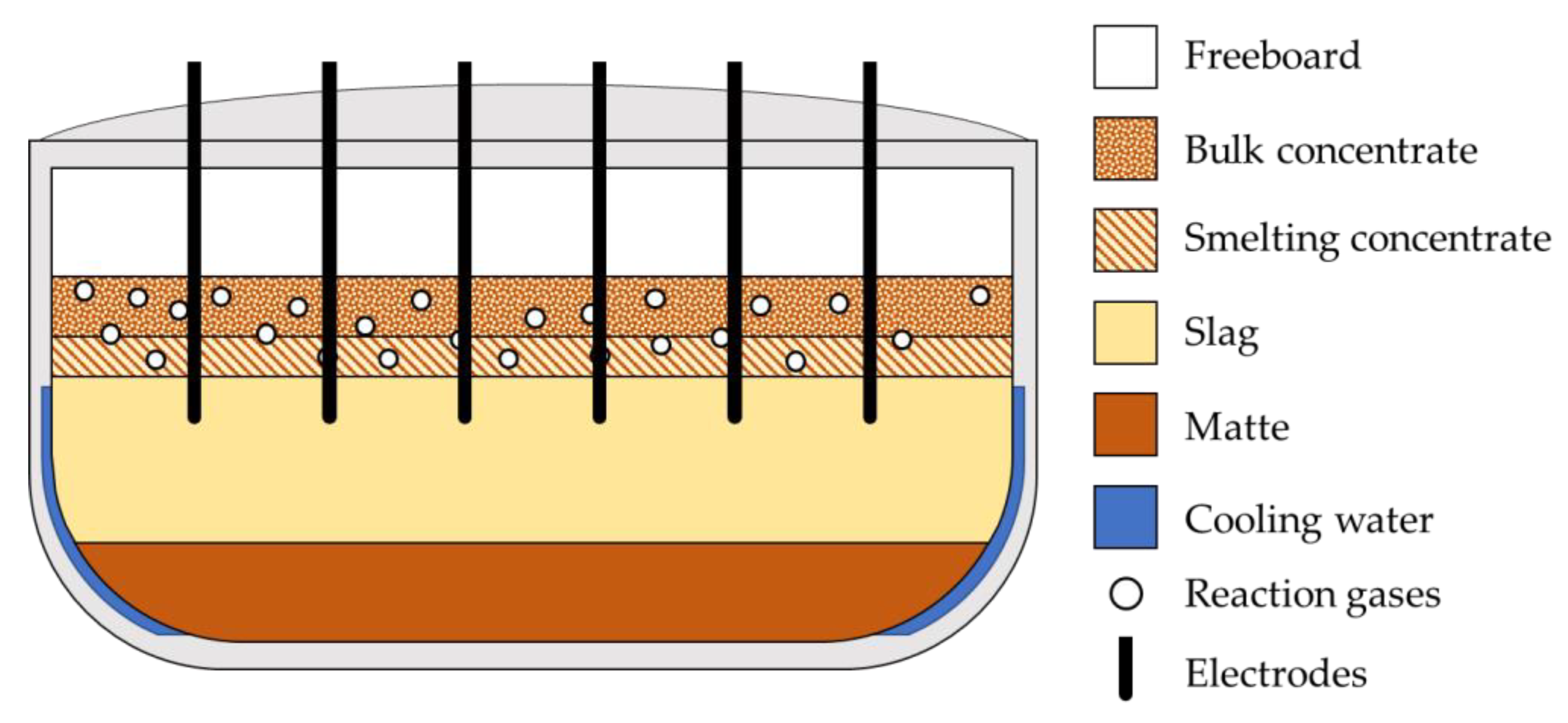
Each of the aforementioned processing steps reduces the bulk of the concentrate or separates gangue from precious metals, increasing the PGM concentration. The smelting step is crucial to the overall PGM extraction process; during smelting, submerged electrode arc furnaces melt dried concentrate into a sulphide matte that acts as a PGM collector, increasing the concentration of PGMs tenfold [2]. The overall viability of the PGM extraction process is therefore reliant on the submerged arc furnaces being operated safely, effectively, and efficiently.

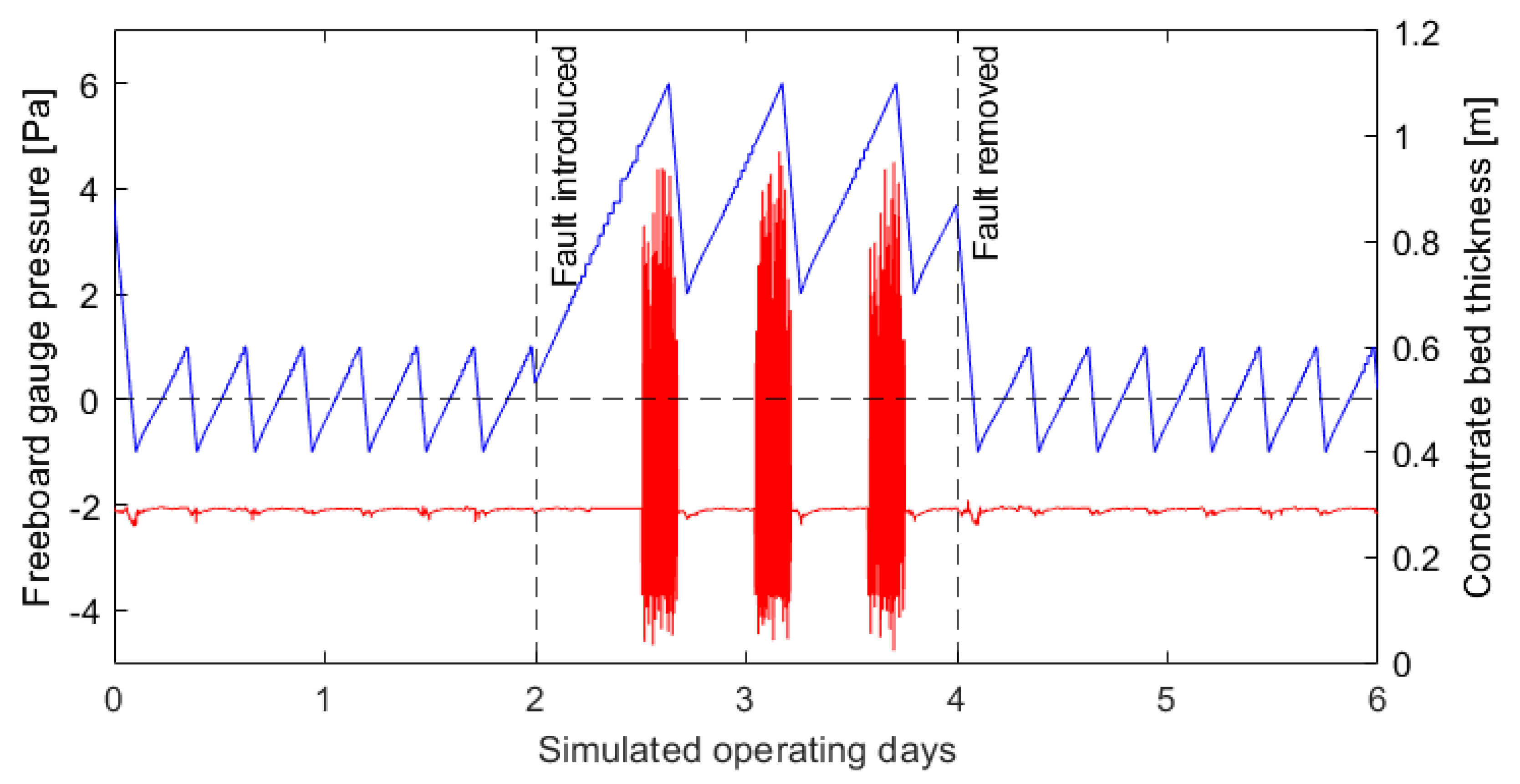
Desulphurization and electrode oxidation reactions within the furnace release sulphur dioxide and carbon monoxide into the furnace freeboard at high temperatures [3], resulting in a freeboard filled with hot, hazardous gases. Freeboard gases are extracted continuously to maintain a negative gauge pressure, preventing these gases from escaping into the surrounding area and jeopardizing operator safety [4]. Atmospheric air drawn in by the negative gauge pressure cools the furnace contents, consequently furnace efficiency is promoted by maintaining the pressure as close to zero as possible.

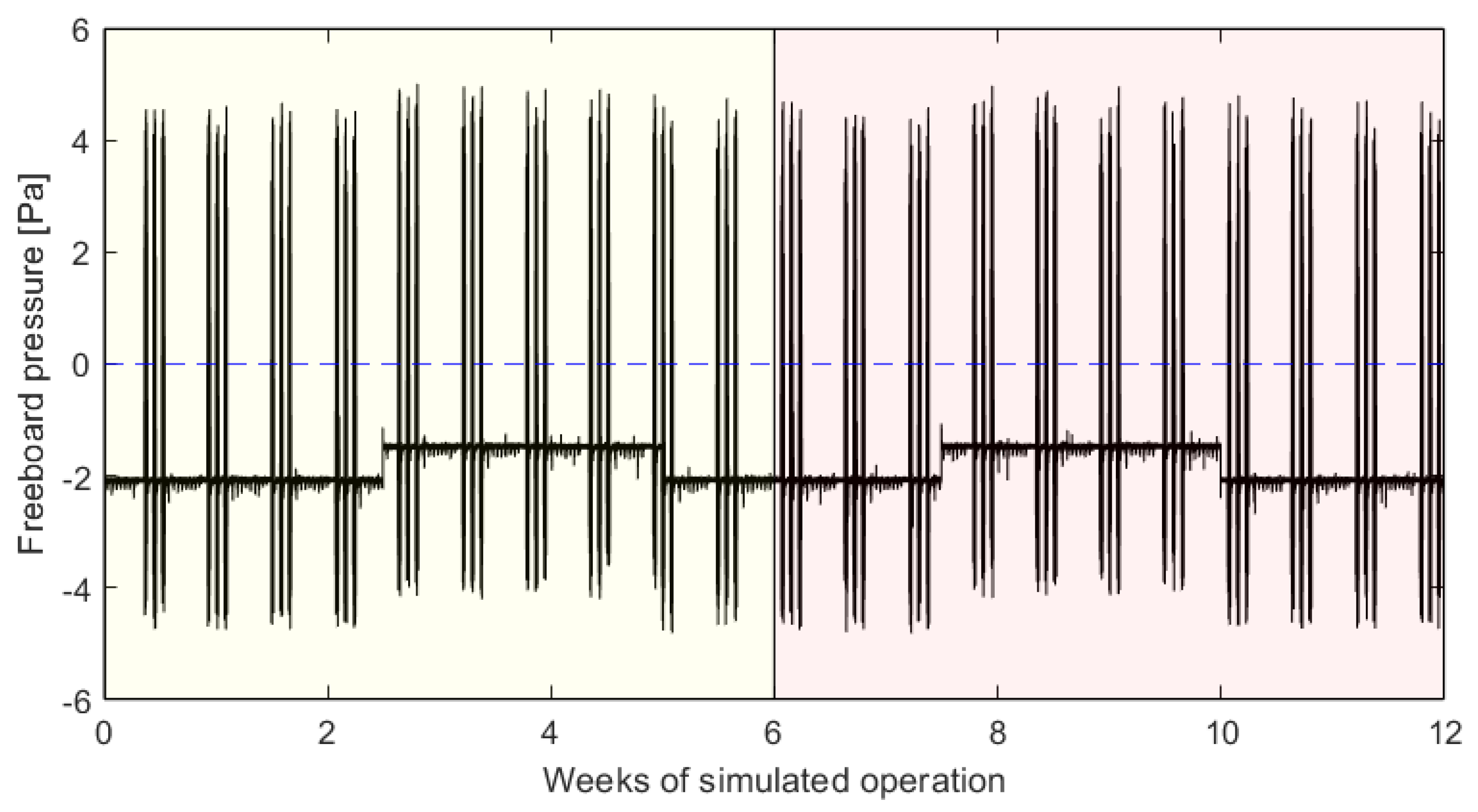
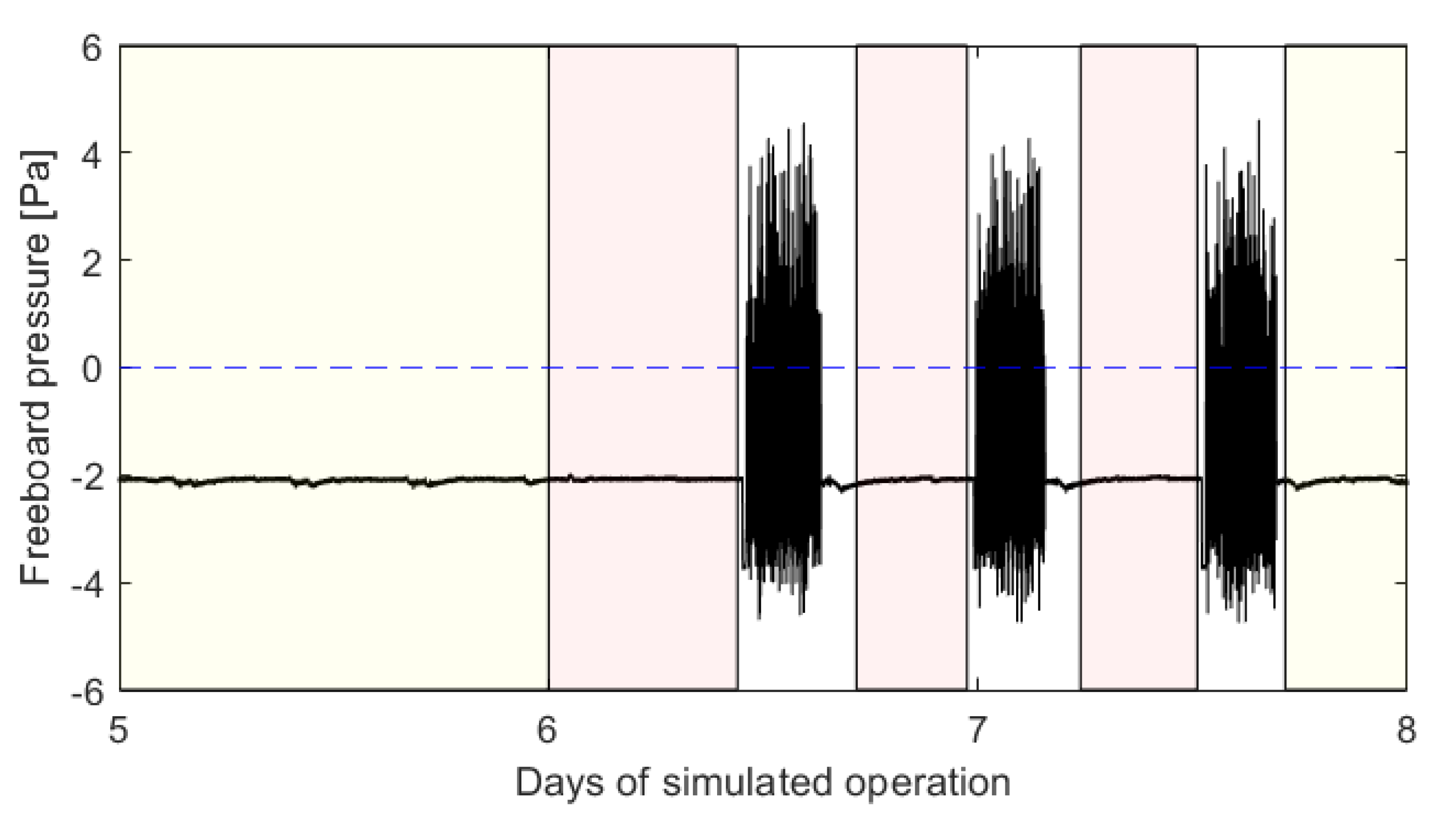
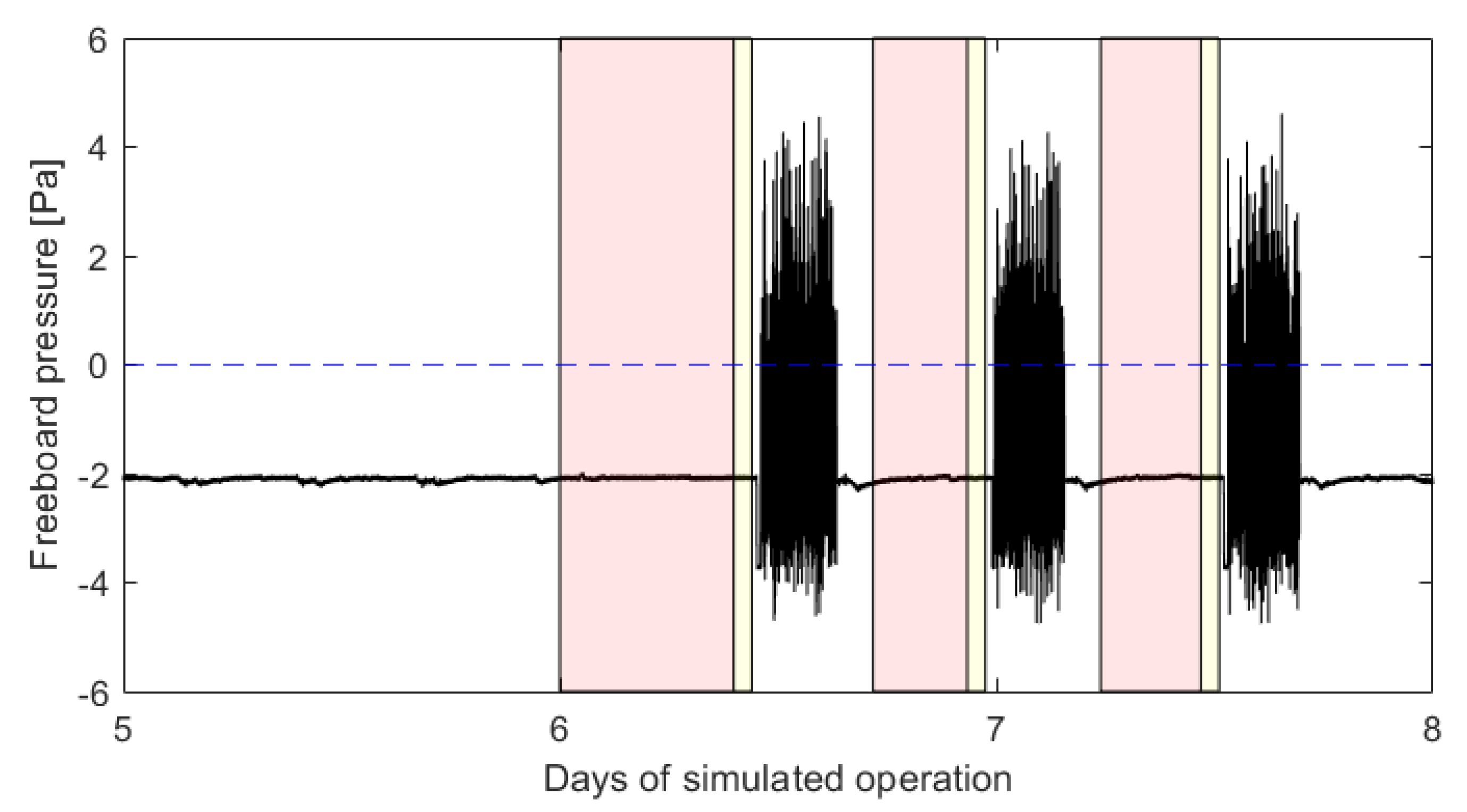
Freeboard pressures can routinely exceed atmospheric pressure despite gas extraction, causing blowbacks. Positive pressure events, also known as blowbacks, occur when hazardous gases escape from industrial furnaces and their causes are unknown. A monitoring model for predicting these events will therefore promote the safety of the smelting operation by providing a warning to operators of impending blowbacks and allow freeboard pressures to be raised when blowbacks are not imminent, promoting efficiency.

Similar to comminution and flotation processes, furnaces are subject to disturbances in the grade and supply of concentrate. These similarities extend to complex process interactions: furnaces are subject to interactions between various furnace zones just as particle interactions, recycle streams, and slurry-air interactions are present and challenging in comminution and flotation process units. Fault conditions in furnaces (i.e., blowbacks), comminution (e.g., mill trips from mill overloading), and flotation (e.g., sliming incidents) can cause sub-optimal operation with potentially rapid and extreme consequences.

Furnaces, as well as the physical mineral processing operations, generate large volumes of historical data. The large data volume recorded from these processes promotes the use of statistical process monitoring for predicting hazardous events such as blowbacks, mill trips, and sliming incidents [5]. This paper evaluates one-dimensional convolutional neural networks as reconstruction-based process monitoring models for predicting blowbacks in industrial submerged arc furnaces. This evaluation will yield insights into the suitability of reconstruction-based monitoring models for predicting hazardous events across the mineral processing chain.

Ideally, historical data recorded from submerged arc furnaces used to develop blowback-prediction models would be completely characterized, i.e., all observations in the historical dataset would be labelled correctly. Models could be trained to predict all possible events from using such a dataset by separating all historical observations into distinct classes [6]. Unfortunately furnace data, like most real-world datasets, are poorly characterized and event-prediction models must be trained using datasets where only a few observations are labelled properly. This constraint has spurred the development of reconstruction-based one-class classifiers as event prediction models [7].

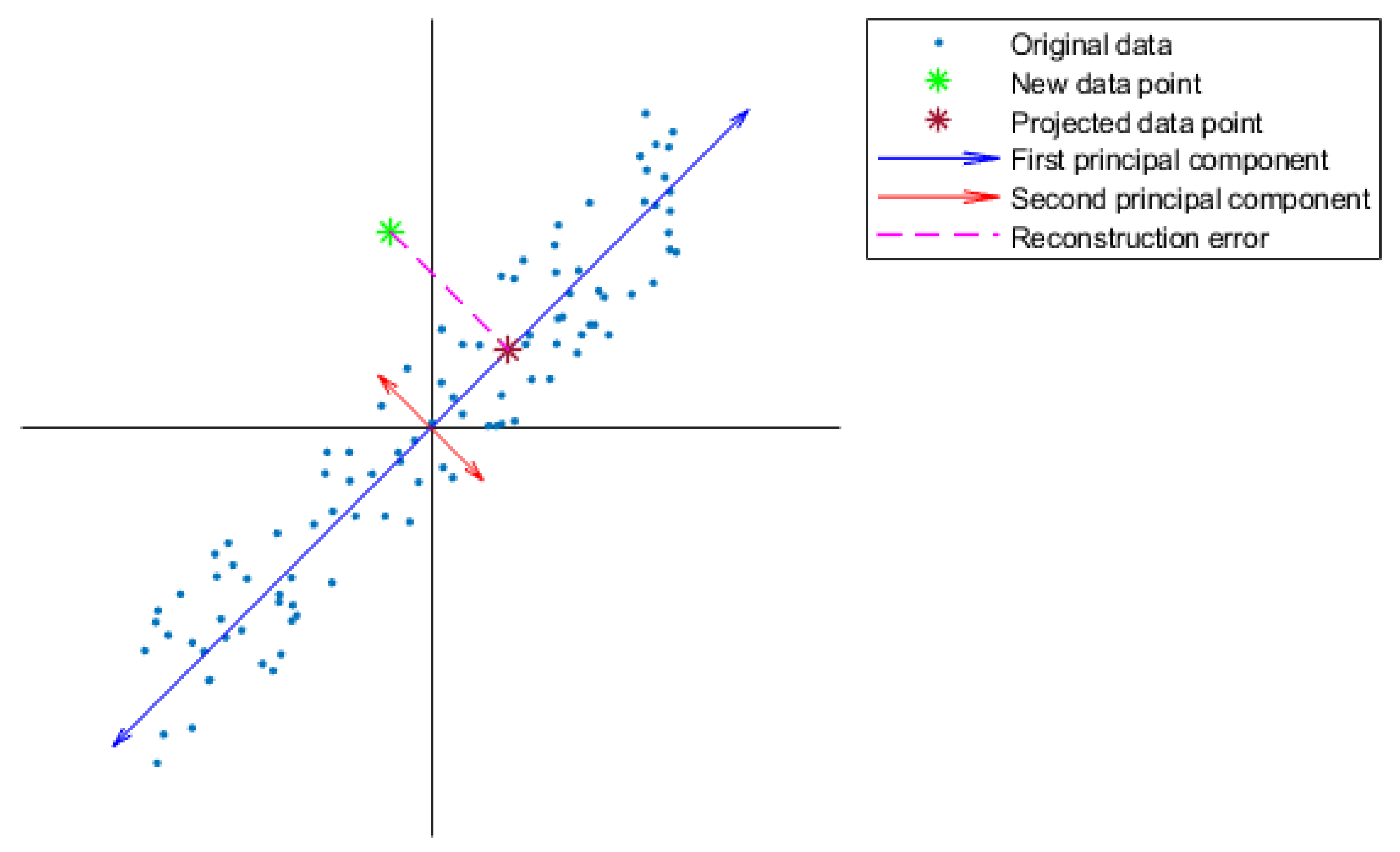
Reconstruction-based one-class classifiers are data-driven models trained to find effective, compressed representations of specific process patterns [8]. If a model is trained to reconstruct the process patterns preceding specific events, then it will reconstruct the specific event-preceding patterns with minimal error. Process patterns that do not precede the target event will be reconstructed inaccurately. This facilitates event prediction based on reconstruction error [9]; lower reconstruction errors suggest that the specific event is imminent, while large reconstruction errors suggest that the event is not imminent. Reconstruction-based event-prediction models are distinguished by how they find compressed representations of process faults.

Principal component analysis (PCA) is the most common approach to feature learning [5,10], and recognizes linear correlations in event-preceding processes [9]. The efficacy of PCA in recognizing specific process patterns has been demonstrated for detecting faults on the Tennessee Eastman simulated process [11], for modelling the normal conditions of batch and continuous chemical processes [12], and for detecting faults in industrial boiler data [13]. Unfortunately, the performance of PCA deteriorates when applied to the nonlinear correlations typically found in industrial data [8], leading to the increasing prominence of neural network-based one-class classifiers.

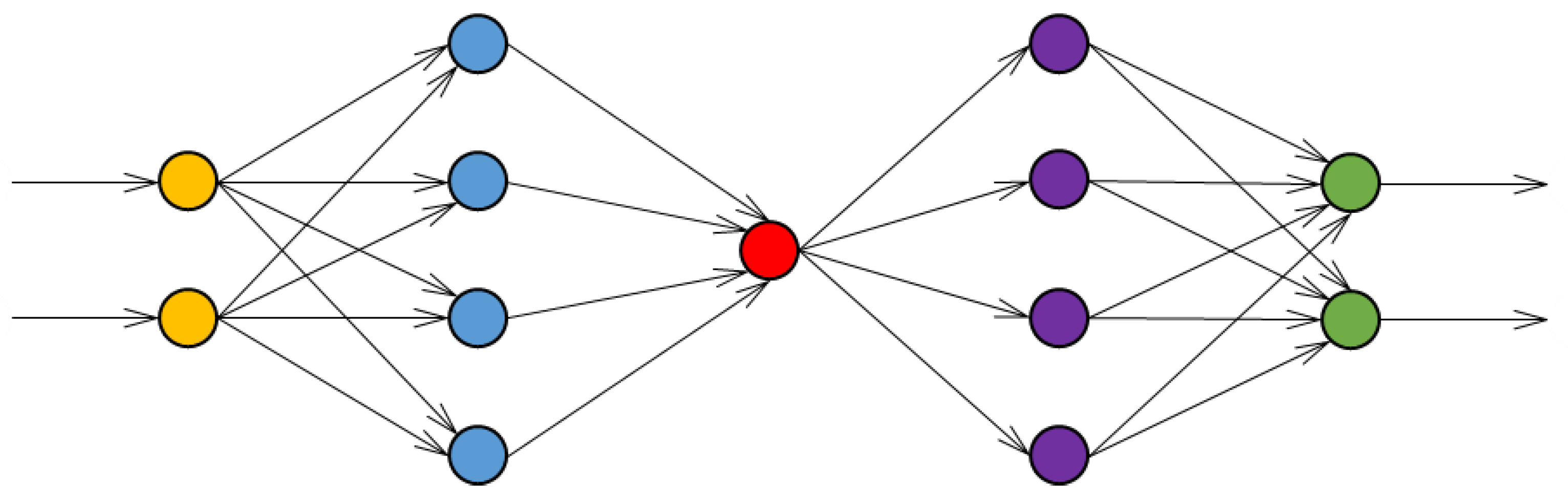
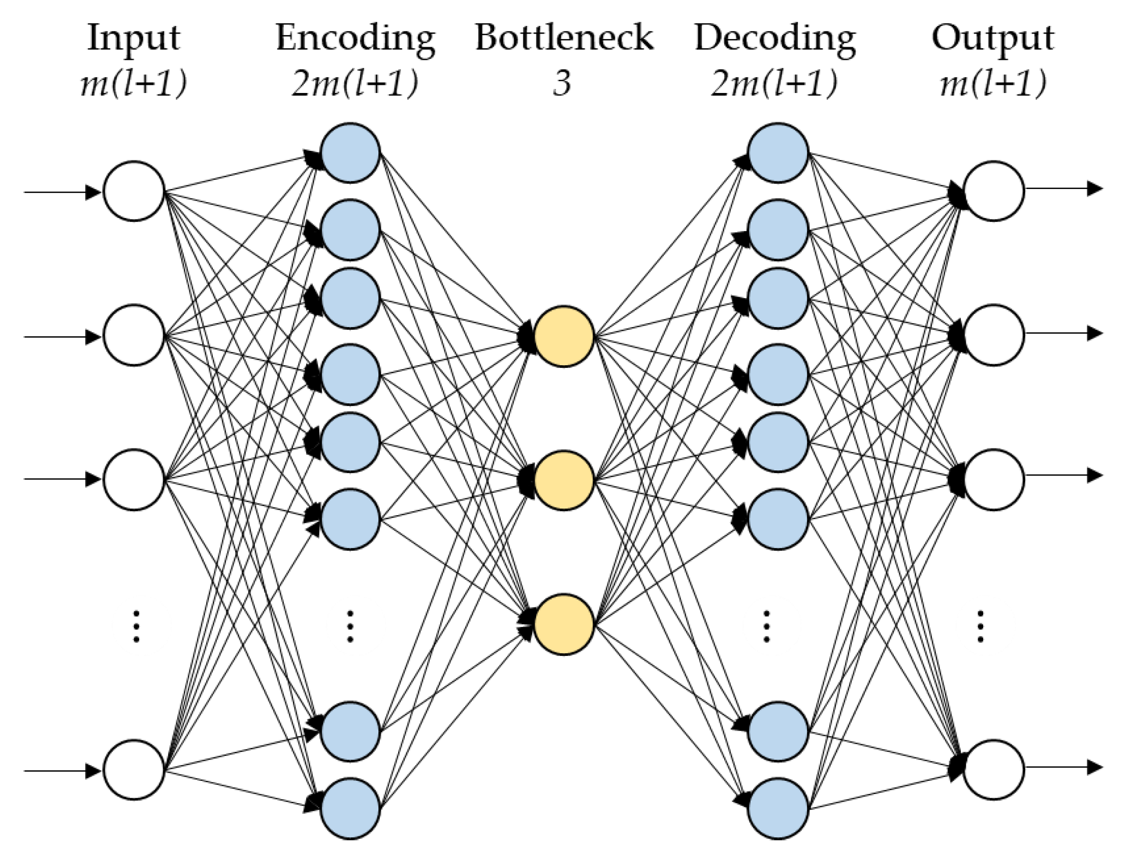
Auto-encoders (AEs) are neural networks that find the low-dimensional subspace that accurately represents network inputs, then reconstruct these inputs as the network outputs. When trained to reconstruct specific event-preceding process patterns they make ideal candidates for reconstruction-based one-class classifiers [10]. Their ability to learn nonlinear representations of industrial process data was demonstrated on the Tennessee Eastman case study [14], and their ability to recognize specific process patterns was demonstrated on a simulated coal mill system [15].

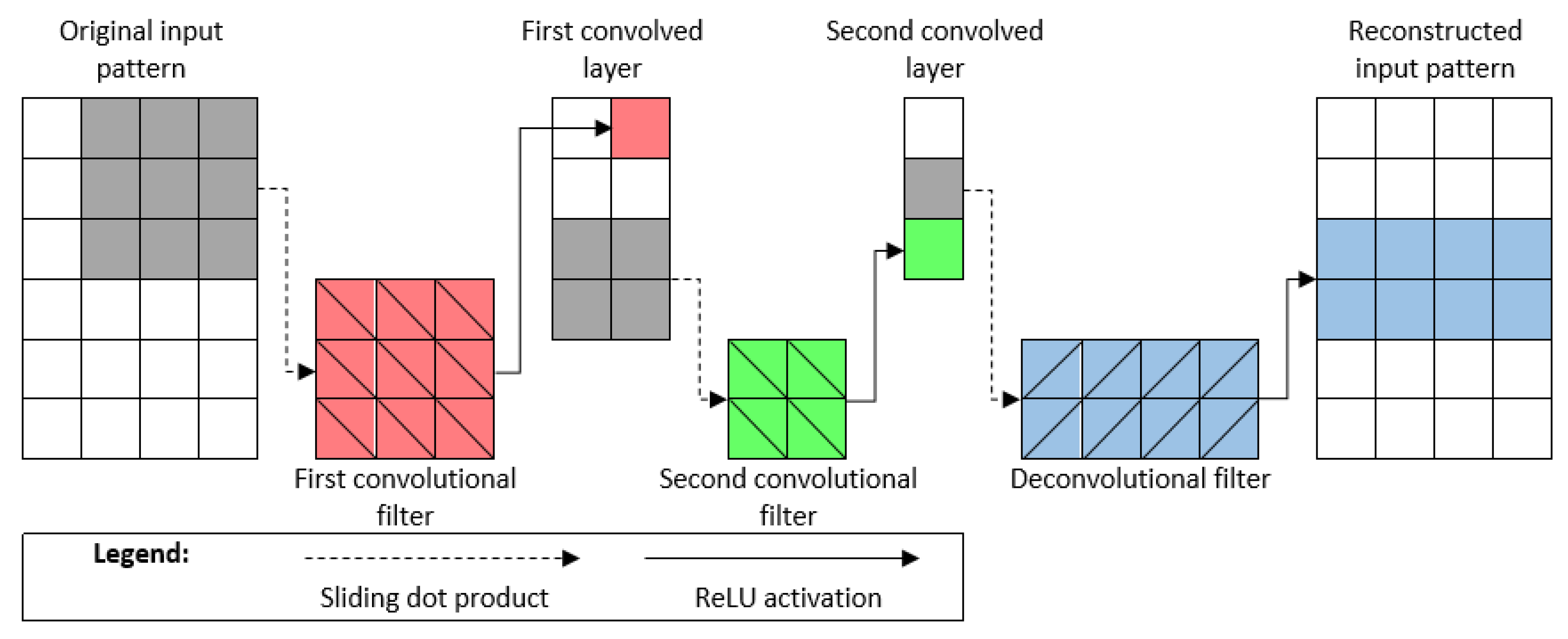
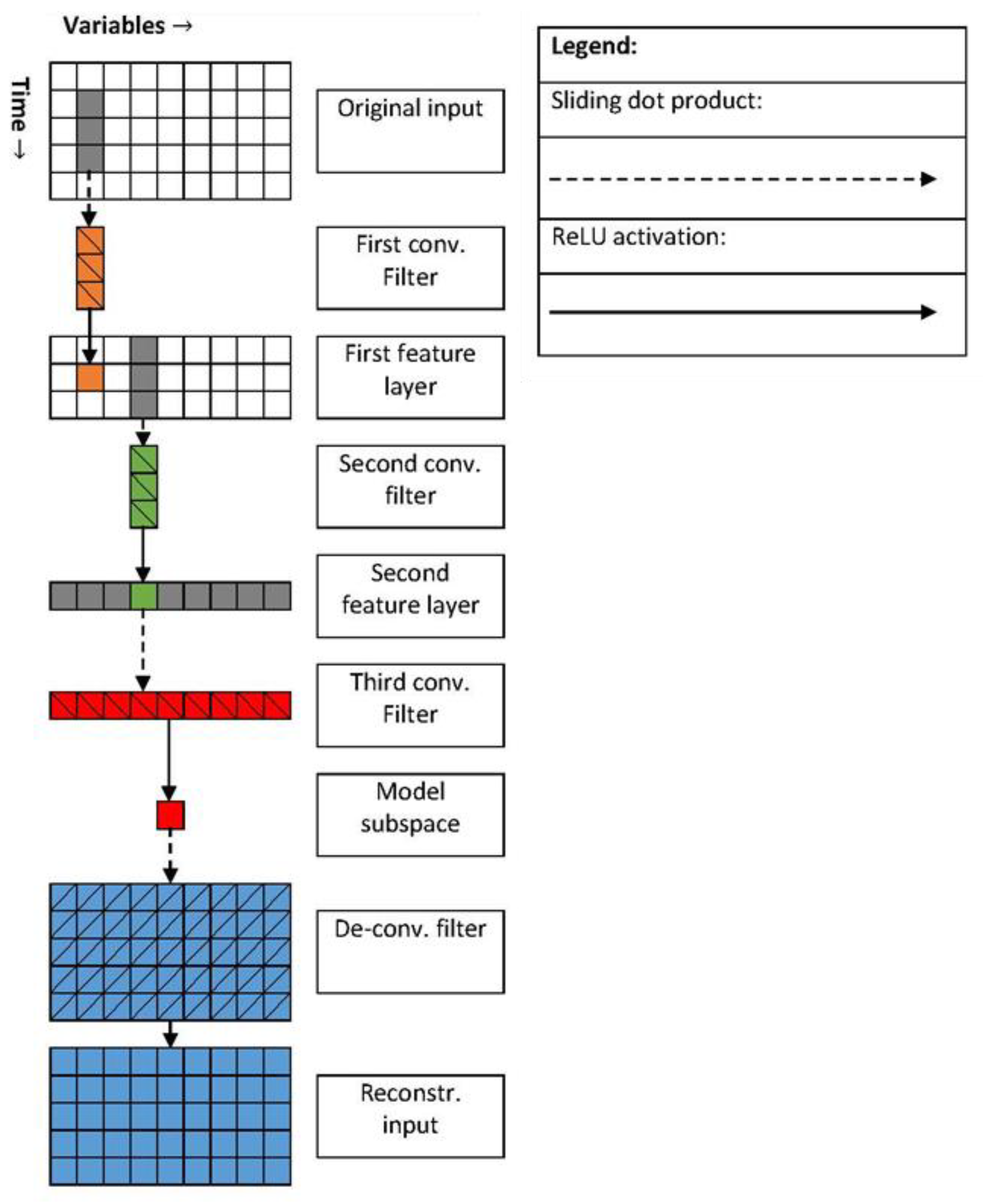
Convolutional neural networks (CNNs) were developed for and completely outclass traditional neural networks in image processing [16]. CNNs extract simple, localized features from network inputs before moving on to more complicated features. This allows for more effective representations of network inputs across convolutional layers [17]. Their adoption for monitoring industrial processes has been slow due to the intrinsic differences between images and multivariate time series, but the localized feature extraction of CNNs can lead to better representations of multivariate time series. Recently, convolutional auto-encoders (CAEs) have been developed for compressing univariate electrocardiogram signals [18] and for fault detection using multivariate time series in the context of process monitoring [19].

This study compares the performance of different reconstruction-based event prediction models using a simulated furnace as case study. The furnace model was developed to specifically account for the complex dynamic interactions in a submerged arc furnace while maintaining a lumped parameter approach to ensure feasible computational costs. Further details on the current study are provided in [20].

2. Methods

2.1. Reconstruction-Based One-Class Classifiers

Data-driven models are used to predict events by applying a model function to monitored process variables. Supervised learning aims to optimally parameterize the model function by minimizing a pre-defined loss function [21,22], but requires labelled observations containing the characteristic patterns preceding the event of interest [23]. Historical datasets are rarely this well-defined, and semi-supervised learning approaches are used to train models using only the historical observations that are known to contain the characteristic patterns. Reconstruction-based one-class classifiers are semi-supervised prediction models that seek to address the problem of ill-defined historical datasets. Three semi-supervised models are considered in this work: principal component analysis, auto-encoders, and convolutional auto-encoders.

In general, model parameters are found by training a model to compress monitored variables $x_i$ to a lower dimensional subspace and to reconstruct the observations accurately [24]. The output of the reconstruction model ${\widehat{x}}_i$ is the reconstructed input, shown in Equation (1).

$${\widehat{x}}_i=f\left(x_i,\mathit{\theta }\right)$$

(1)

Using Equation (1), a model function, $f$, with model parameters, $\mathit{\theta }$, is applied to an observation of multiple variables, $x_i$. The model is trained on historical observations that are known to contain the event-preceding patterns, and, if properly trained, will reconstruct all observations with the characteristic patterns accurately while reconstructing those without inaccurately. The reconstruction error, ${\epsilon }_{R,i}$ quantifies how accurately an observation $x_i$ is reconstructed (Equation (2)):

$${\epsilon }_{R,i}=\Vert x_i-{\widehat{x}}_i{\Vert }^2$$

(2)

The inverse of ${\epsilon }_{R,i}$, $u_i=1/{\epsilon }_{R,i}$, can be used as a discriminant. Higher discriminant values suggest that the reconstructed observation is similar to the observations used to train the reconstruction model. Therefore, the reconstruction model will generate higher discriminant values on observations that precede specific events if it was trained on those events. The reconstruction model is semi-supervised because it does not require negative samples during training, i.e., observations outside the target event [21].

Equation (3) formally states the training algorithm used to obtain reconstruction model parameters, $\mathit{\theta }$, from observations in the historical data, $X_t$, where $X_t$ is the subset of datapoints preceding the event to be predicted.

$$\mathit{\theta }=\underset{\mathit{\theta }}{\mathrm{argmin}}\left(ℰ\left(f,\mathit{\theta },X_t\right)\right)=\underset{\mathit{\theta }}{\mathrm{argmin}}\left({\displaystyle \sum }_i\Vert x_i-f\left(x_i,\mathit{\theta }\right){\Vert }^2\right)$$

(3)

The generated discriminant values are compared to a recognition threshold before making a prediction. However, a theoretical basis for the reconstruction recognition threshold does not exist, and has to be obtained empirically [8].

The reconstruction-based model is trained by minimizing Equation (2) over all training samples, and is therefore sensitive to the units of variables in each observation [8]. Each observation is therefore standardized (rescaled to zero mean and unit variance) before the model is trained. Inputs can be corrupted during training by adding normally distributed noise with zero mean and variance ${\sigma }_C^2$ to each observation, then training the model to reconstruct the original, uncorrupted input, improving model generalizability [15]. This is illustrated in Equation (4), where variable $j$ of a standardized observation $z_i$ is corrupted with normally distributed noise. The variance ${\sigma }_C^2$ represents an additional design parameter that must be specified before model parameters can be derived.

$${\widehat{z}}_{i,j}=z_{i,j}+\mathcal{N}\left(0,{\sigma }_C^2\right)$$

(4)

2.1.1. Principal Component Analysis

Principal component analysis (PCA) is a prominent data-driven model applied in process monitoring. Using PCA, the directions of significant linearly uncorrelated variance are identified using recorded data of specific process conditions [25]. These directions constitute a linear subspace of target process conditions and are called the principal components of the modelled data. Observations with similar correlation structures to the target process conditions are well represented in this subspace and can be reconstructed accurately; therefore, PCA is an ideal model to recognize process conditions characterized by distinct linear correlation structures [9]. Figure 1 provides an illustration of PCA-based reconstruction.

Linear correlations between variables are well-approximated in the PCA subspace, but this subspace excludes autocorrelations between observations. PCA is therefore best suited for static processes [11,24]. Dynamic PCA (dPCA) is a simple modification of PCA that addresses this limitation. Using dynamic PCA, observations are lagged, incorporating previous values in each observation as shown in Equation (5), allowing PCA to include autocorrelations in its subspace [11,26]:

$$x_i^L=\left[x_i x_{i-1} x_{i-2}\cdots x_{i-\left(l-2\right)} x_{i-\left(l-1\right)} x_{i-l}\right]$$

(5)

2.1.2. Auto-Encoders

Auto-encoders (AEs) are feedforward neural networks that find effective representations of inputs and reconstruct them accurately [8]. Like neural networks, AEs have network architectures consisting of layers of neurons with weighted connections. What distinguishes AEs is their equally sized input and output layers and the existence of a bottleneck layer. The bottleneck layer has fewer neurons than the input and represents the nonlinear subspace of modelled data [8]. Figure 2 illustrates a typical AE network architecture. The neurons in an AE function similarly to those in standard neural networks, where each neuron accepts weighted inputs and biases to produce an output dependent on the selected (often nonlinear) activation function [27].

Gradient-based optimization routines are used to determine the parameters which satisfy Equation (3). Early nonlinear activation functions used in neural networks, like sigmoid and hyperbolic tangent functions, struggled with vanishing gradient problems, posing serious problems to gradient-based optimization [28]. The Rectified Linear Unit (ReLU) activation function (Equation (6)) is frequently used to overcome this problem. To avoid convergence to local minima, the gradient descent with momentum algorithm (Equation (7)) is often used to train neural networks [22]. At each iteration, $k$, a weight $w\in \mathit{\theta }$ is updated based on how much it contributed to the overall loss function according to the learning parameter $\eta$. The third term introduces momentum using the parameter $\gamma$ to increase the likelihood that the model will find globally optimized weights and biases. Lastly, regularization is used to modify the error function [22]. Using $L_2$-regularization (equation 8), over-fitting can be avoided by adjusting the penalty parameter $\lambda$ controlling the degree of regularization; larger values of $\lambda$ results in more regularized model parameters.

$${\varphi }_{ReLU}\left(x\right)=\max \left(x,0\right)$$

(6)

$$w_{k+1}=w_k-\eta \left(\frac{\partial ℰ\left(X_t,{\widehat{X}}_t\right)}{\partial w_k}\right)+\gamma \left(w_k-w_{k-1}\right)$$

(7)

$$ℰ{\left(X_t,\mathit{\theta }\right)}_{L_2}=ℰ\left(X_t,\mathit{\theta }\right)+\frac{\lambda }{2}\Vert \mathit{\theta }{\Vert }^2$$

(8)

Auto-encoders are able to identify nonlinear characteristics between variables in each observation but, like PCA, are unable to identify dynamic characteristics between observations. As with PCA, observations can be lagged to incorporate previous values in each observation using Equation (5).

2.1.3. Convolutional Auto-Encoders

Convolutional auto-encoders (CAEs) are not fundamentally different from typical AEs. In fact, CAEs can be seen as a special case of fully-connected AEs [22]. They use the same activation functions and can both be trained using backpropagation combined with gradient descent algorithms. Convolutional auto-encoders are distinguished by the use of convolutional layers. Figure 3 provides an illustration of a simple CAEs architecture typically used in applications with two-dimensional data sets (e.g., images). The neurons in convolutional layers are connected to a subset of the neurons in the preceding layer. These subsets (shaded grey in Figure 3) are simpler than the set of all outputs from the preceding layer, and are connected by far fewer weighted connections [27].

2.2. Case Study

The proposed event prediction methods were evaluated using a simulated submerged arc furnace with dynamic characteristics as a case study. The hazardous events simulated by the furnace model are positive pressure events (PPEs). The freeboards of submerged arc furnaces contain hazardous gases such as carbon monoxide at high temperatures [29,30]. A negative freeboard gauge pressure is maintained to prevent these gases from escaping. PPEs occur when the gauge pressure of the furnace freeboard becomes positive, releasing hazardous gases into the surroundings. Figure 4 shows the layout of the furnace model simulation. The full model derivation and implementation is presented in [20].

The dynamic furnace model is derived by performing mass and energy balances over distinct zones of the furnace interior (Figure 4) to obtain a set of ordinary differential equations. This set of ordinary differential equations is used to generate datasets on which to evaluate the PPE prediction models [20]. These datasets are created by sampling the furnace model variables that can be monitored in a submerged arc furnace. The list of monitored variables is given in

Table 1. Monitored variables in the simulated dataset.

	Monitored Variable	Symbol	Units
1	Slag zone height	$L_S$	$\mathrm{m}$
2	Matte zone height	$L_M$	$\mathrm{m}$
3	Slag zone temperature	$T_S$	$\mathrm{K}$
4	Matte zone temperature	$T_M$	$\mathrm{K}$
5	Bulk concentrate temperature	$T_{C\left(B\right)}$	$\mathrm{K}$
6	Freeboard temperature	$T_G$	$\mathrm{K}$
7	Cooling water temperature	$T_W$	$\mathrm{K}$
8	Freeboard pressure	$C_{G,R}$	$\mathrm{Pa}$
9	Reaction gas concentration in freeboard	$P_G$	$\mathrm{mol}/{\mathrm{m}}^3$

.

The generated datasets correspond to 12 weeks of simulated operation [20]. Each monitored variable is sampled once every ten seconds; the resulting dataset contains $n~$ 726,000 observations and $m=$ 9 features (Table 1). The simulation switched between two modes of operation; one where the furnace is operated in a way that does not cause PPEs, and one where the furnace is operated in a way that causes PPEs.

PPEs are caused in the furnace model by increasing the concentrate bed thickness. During normal operation, the concentrate feed rate to the furnace is manipulated so that the bed thickness is maintained between 0.4 m and 0.6 m. PPEs occur by manipulating the feed rate so that the thickness varies between 0.7 m and 1.0 m. This causes reaction gases to build up in the concentrate, causing the bed to rupture and reaction gases to release rapidly into the freeboard. The effect of concentrate bed thickness is shown in Figure 5.

2.3. Performance Evaluation

Evaluating the reconstruction-based event prediction models presented in this work requires that prediction performance metrics be defined.

Table 2. Possible outcomes when a predictive model is applied to an observation in a confusion matrix.

	Pattern Present	Pattern Absent
Recognition	True positives— $TP$	False positives— $FP$
No recognition	False negatives— $FN$	True negatives— $FN$

defines the four possible outcomes when a predictive model is applied to an observation in a confusion matrix [31].

The outcomes given in Table 2 are converted into metrics that express predictive performance from different perspectives. Typically, a classifier should have good sensitivity $\varphi$ (Equation (9)) as well as specificity $\psi$ (Equation (10)) [31].

$$\varphi =\frac{TP}{TP+FN}$$

(9)

$$\psi =\frac{TN}{TN+FP}$$

(10)

Specificity indicates how well a model flags negative samples as such, while sensitivity shows how well a model flags positive samples. While specificity and sensitivity express model performance from different perspectives, they can give misleading impressions of model performance in unbalanced datasets. Precision (given in Equation (11)) is a useful performance metric for datasets with few positive samples and many negative samples, as it indicates the probability that a prediction made by a model is correct:

$$\phi =\frac{TP}{TP+FP}$$

(11)

While a high precision shows that a model makes predictions with very few false alarms, it does not show how quickly that model makes those predictions, or if those predictions precede events with enough time to be useful. Time-to-event $\Delta t_{TE}$ (Equation (12)) expresses how quickly a model recognizes an event-preceding pattern before that event occurs:

$$\Delta t_{TE}=t_{event}-t_{detection}$$

(12)

2.4. Data Partitioning

A fair evaluation of the performance of a data-driven predictive model requires that the model be tested on data other than the training data. The simulated data with $n$ observations and $m$ features generated by the furnace model ($Xϵ{ℝ}^{n\times m}$) is partitioned into training ($X_0ϵ{ℝ}^{n_0\times m}$) and testing ($X_1ϵ{ℝ}^{n_1\times m}$) datasets. This partitioning is shown in Figure 6, where 12 weeks of simulated data is partitioned into training (gold) and testing (red) datasets.

Reconstruction-based event prediction models should only be trained on data where the characteristic patterns that precede the target event are present. Therefore, a target dataset ($X_tϵ{ℝ}^{n_t\times m}$) is constructed from a subset of observations in $X_0$. The ground truth regarding the presence of faulty conditions of the simulated data is known and is illustrated in Figure 7. The areas shaded in red shows where the PPE-causing fault is present, and gold-shaded areas indicate its absence. Note that the PPE-causing fault is present in unshaded areas in Figure 7, but detection at this point in time would not provide sufficient response time to operators before the target event occurs for the prediction to be useful.

Unfortunately, the ground truth in industrial datasets is rarely known. However, the hazardous event is easily identified and training samples for a reconstruction-based event prediction model can be selected from a window preceding the target event [31]. Therefore, a prediction is assumed to be valid for a time ($\Delta t_{prediction}$) preceding the event. The prediction is correct if the event occurs within this period, and if enough time ($\Delta t_{warning}$) is available to take corrective measures. These two metrics allow a window of training samples that precede each event to be defined as illustrated in Figure 8:

Specifying $\Delta t_{prediction}$ and $\Delta t_{warning}$ defines a window preceding each event in the training dataset where predictions would be valid. Training samples can then be selected from these windows in the training dataset. Figure 9 illustrates observations in $X_0$, highlighted in gold, that are selected as training samples for $\Delta t_{prediction}=1.5\mathrm{h}$ and $\Delta t_{warning}=0.5\mathrm{h}$. These training samples are used to construct a new target dataset, $X_t$.

Note that $X_t$ does not contain all observations in $X_0$ where the event-preceding patterns are present; the above approach is simply a way of selecting observations with patterns that, if recognized, will flag the observations that precede each event. Recognitions immediately succeeding these observations will not reduce model specificity nor increase specificity despite the presence of the characteristic patterns that precede the PPEs; they do not provide sufficient warning time before the PPEs.

2.5. Model Development

Model parameters for the dPCA, AE, and CAE models are derived from the synthetically generated dataset.

Table 3. Model derivation algorithm for dPCA.

	Step Description	Output	Equation
1	Standardize $X_t$	$Z_t$	-
2	Lag the standardized dataset $Z_t$	$Z_t^L$	5
3	Optimize model parameters to reconstruct $Z_t^L$ from ${\widehat{Z}}_t^L$	$V$	3

shows the model derivation algorithm for the dPCA model, while

Table 4. Model derivation algorithm for both AE and CAE.

	Step Description	Output	Equation
1	Standardize $X_t$	$Z_t$	-
2	Lag the standardized dataset $Z_t$	$Z_t^L$	5
3	Construct corrupted $Z_t^L$	${\widehat{Z}}_t^L$	4
4	Optimize model parameters to reconstruct $Z_t^L$ from ${\widehat{Z}}_t^L$	$\mathit{\theta }$	3

shows how the AE and CAE models are derived. Finally,

Table 5. dPCA, AE, and CAE application algorithm.

	Step Description	Output	Equation
1	Standardize $x_i$	$z_i$	-
2	Lag $z_i$ with $l$ observations	$z_i^L$	5
3	Reconstruct $z_i^L$	${\widehat{z}}_i^L$	1
4	Calculate the reconstruction error	${\epsilon }_i^R$	2

shows how the derived models are used to calculate the reconstruction error for new observations.

2.5.1. Dynamic Principal Component Analysis

The principal components of a dataset, $X_tϵ{ℝ}^{n\times m}$, are computed through eigenvalue decomposition of the covariance matrix of the dataset. This is shown in Equation (13) below:

$$X^{T}X{v}_j={\lambda }_j{v}_j$$

(13)

where $v_jϵ{ℝ}^{m\times 1}$ is a principal component of $X$. The corresponding eigenvalue, ${\lambda }_j$, is the total variance captured on this principal component. A PCA subspace is constructed using the most significant principal components, i.e., the components with the most variance. The significance of $v_j$ is expressed by the fraction of total variance captured [32]. This fraction is calculated using Equation (14).

$${\eta }_j=\frac{{\lambda }_j}{{\sigma }_X^2}=\frac{{\lambda }_j}{{{\displaystyle \sum }}_{j=1}^m{\lambda }_j}$$

(14)

where ${\sigma }_X^2$ is the total variance in $X$. The PCA subspace, $Vϵ{ℝ}^{m\times v}$, contains the $v$ most significant components. Retaining insignificant components causes noise to be retained in the PCA subspace. Selecting the optimal number of retained components, v, is therefore crucial to dPCA modelling [32]. In this investigation, $v$ is selected so that 99.9 % of the variance in the training set is retained. The reconstruction model for dPCA, $f_{PCA}$, is given by Equation (15) below:

$${\widehat{x}}_i=f_{PCA}\left(x_i,V\right)=x_{i}V{V}^{\mathrm{T}}$$

(15)

2.5.2. Auto-Encoder

The auto-encoder network architecture used in this investigation follows the template shown in Figure 10. Each observation with $m$ features is lagged $l$ times, requiring $m\left(l+1\right)$ input- and output neurons. The encoding and decoding layers contain twice as many neurons as the input and output layers. This investigation considers an auto-encoder with three neurons in the hidden bottleneck layer.

Equation (11) is used to determine the number of network parameters (weights and biases) to be learnt iteratively using the gradient descent with momentum algorithm. This equation uses a dataset with $m$ = 9 features lagged $l$ = 4 times. Using equation 16, it is demonstrated that the auto-encoder used in this investigation has 8958 learnable parameters.

Table 6. AE design parameters.

	Design Parameter	Investigated Value
1	Network architecture, $f\left(x_i,\mathit{\theta }\right)$	See Figure 10
2	Lag dimension, $l$	4
3	Input corruption variance, ${\sigma }_C^2$	0.1
4	Number of bottleneck neurons, $N_{hidden}$	3
5	Regularization parameter, $\lambda$	${10}^{-5}$
6	Learning rate, $\eta$	0.01
7	Momentum parameter, $\gamma$	0.001

shows the design parameters specified for the auto-encoder before model parameters are derived through training.

$$N_{\mathit{\theta }}=4{\left(m\left(l+1\right)\right)}^2+4N_{hidden}m\left(l+1\right)+4m\left(l+1\right)+N_{hidden}$$

(16)

2.5.3. Convolutional Auto-Encoder

Figure 11 shows the convolutional auto-encoder network architecture used in this investigation. Each input is a $5\times 9$ matrix; $m$ = 9 features, each lagged $l$ = 4 times. The first two convolutional filters have a $3\times 1$ dimension and will therefore only convolve across the time dimension. The first two convolutions eliminate the time dimension, yielding a $1\times 9$ convolved feature. The third convolutional layer convolves across the variables, yielding the model subspace of single values. It is from this model subspace that the original input is reconstructed using a $5\times 9$ deconvolutional filter.

Table 7. CAE network parameters in the investigated CAE architecture.

	Layer Type	Output Size	Filter Shape	No. of Filters	Parameters
1	Input	$5\times 9\times 1$
2	Convolution + ReLU	$3\times 9\times 8$	$3\times 1$	$8$	24 weights, 8 biases
3	Convolution + ReLU	$1\times 9\times 8$	$3\times 1$	$8$	192 weights, 8 biases
4	Convolution + ReLU	$1\times 1\times 4$	$1\times 9$	$4$	288 weights, 4 biases
5	Deconvolution	$5\times 9\times 1$	$5\times 9$	$1$	252 weights, 1 bias
6	Output	$5\times 9\times 1$

shows how many convolutional filters are used at each layer, as well as how many learnable parameters exist for each filter. The table quantifies the complexity of the investigated convolutional auto-encoder architecture. It shows that the architecture only has 707 learnable parameters.

3. Results and Discussions

The performances of the evaluated reconstruction-based models are closely linked to the recognition thresholds at which they are evaluated. However, these thresholds can be selected arbitrarily. Therefore, each model will be evaluated at three different thresholds shown in

Table 8. Recognition thresholds selected for model evaluation.

	Recognition Threshold	Motivation
1	Threshold where 95% precision is achieved.	Useful to evaluate detection delay and specificity at high precision
2	Maximum threshold where all PPEs are predicted.	Enables prediction of each blowback
3	Minimum threshold where 100% specificity is achieved.	No false alarms

, as well as the motivation for using these thresholds for evaluation.

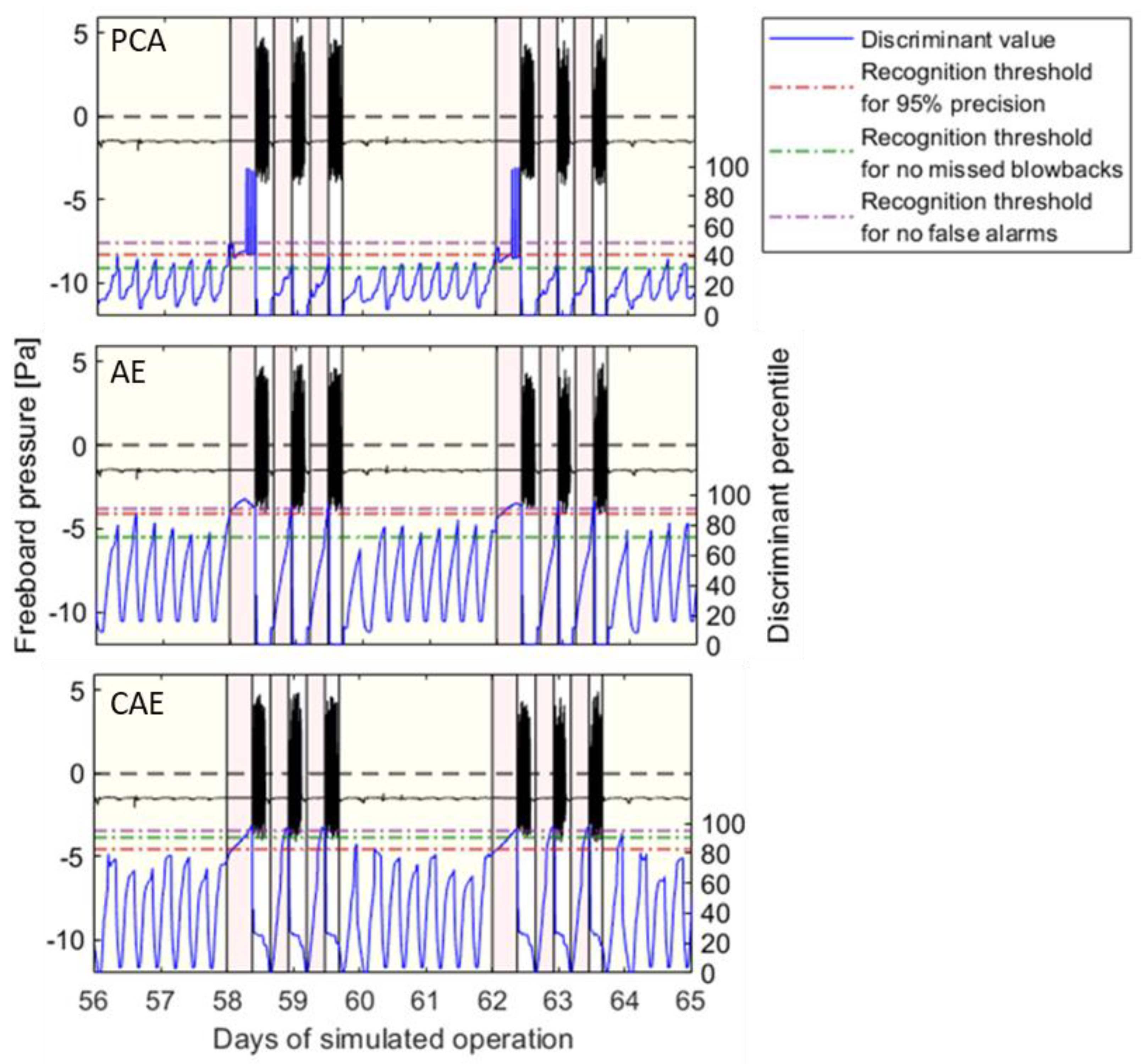
Figure 12 shows the discriminant values generated by each of the investigated models over 9 days of simulated operation. Note that this evaluation is performed over 42 days of simulated operation; these figures are only for illustrative purposes. These figures also show the recognition thresholds given in Table 8.

Figure 12 shows that the dPCA, AE, and CAE models are all unable to achieve both zero missed predictions and perfect specificity: the recognition threshold for no false alarms is greater than that for no missed blowbacks for each model.

Table 9. Event prediction performance at different prediction thresholds for dPCA, AE, and CAE.

95 % Precision:		dPCA	AE	CAE
1	Average time-to-event (hrs)	3.08	2.65	4.43
2	Sensitivity (%)	24.73	27.80	52.12
3	Specificity (%)	99.49	99.40	98.99
4	Failed predictions	40	20	0
	No failed predictions:	dPCA	AE	CAE
5	Average time-to-event (hrs)	3.99	4.06	2.29
6	Sensitivity (%)	43.94	46.23	24.95
7	Specificity (%)	86.70	90.14	99.86
8	Failed predictions	0	0	0
	No false predictions:	dPCA	AE	CAE
9	Average time-to-event (hrs)	1.45	2.24	1.26
10	Sensitivity (%)	2.39	22.18	11.37
11	Specificity (%)	100.00	100.00	100.00
12	Failed predictions	46	24	16

shows the event prediction performance metrics at 95% precision, no missed alarms, and perfect specificity for each investigated model, respectively.

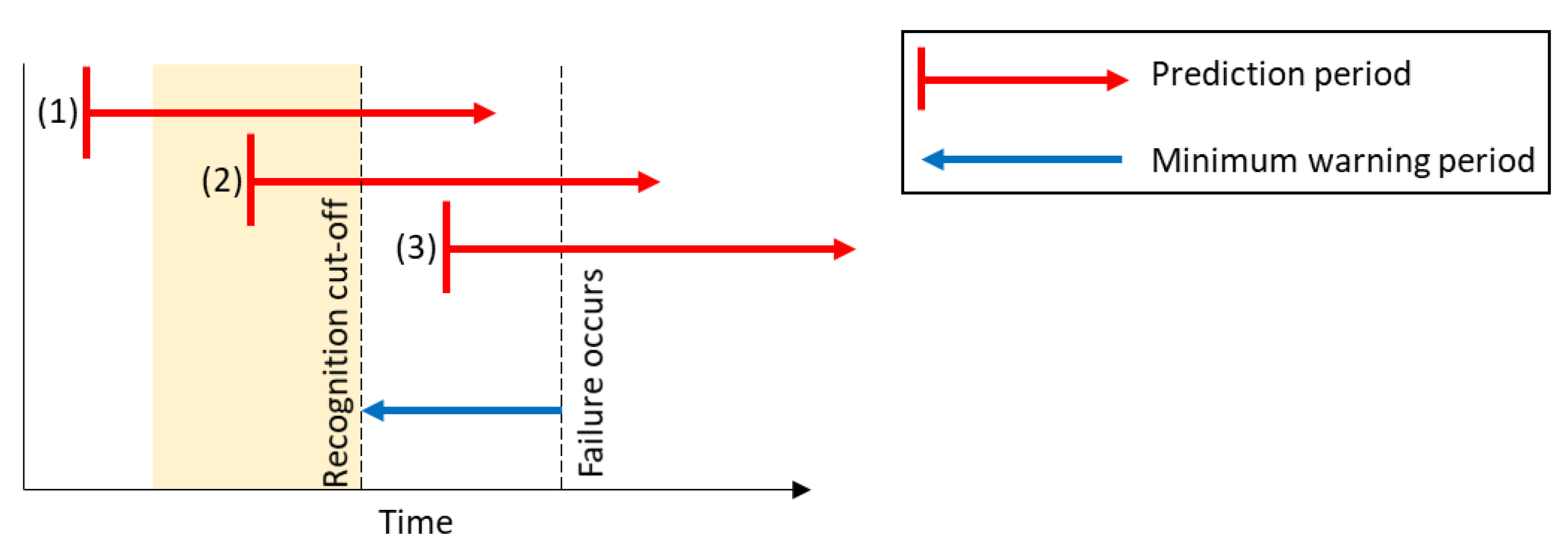
Note that sensitivity refers to the fraction of all observations that precede events that is recognized by the predictive models. The number of failed predictions is the number of the predictive models failed to recognize a single observation in the windows preceding the target events. Therefore, a model can have a sensitivity lower than 100% while still succeeding in predicting each event.

The results presented in Table 9 suggests that the performance of the CAE model, relative to the AE- and dPCA models, is superior in the case study evaluated in this work.

Entry 1 in Table 9 show that the CAE model correctly recognized event-preceding conditions more quickly than the dPCA and AE models when the recognition threshold is set so that the precision of each model in recognizing event-preceding conditions is 95%. Furthermore, entry 4 shows that the CAE model managed to predict each event, while the AE- and dPCA models failed to predict 20 and 40 blowbacks out of 63, respectively.

While inferior to the CAE model at the 95% precision threshold, the nonlinear AE model did manage to outperform the linear dPCA model. The dPCA model did show lower average detection delays than the AE model (as seen in entry 1 in Table 9) but failed in predicting events twice as often. This suggests that predictions based solely on a process’ linear characteristics will struggle to compete with predictions that utilize nonlinear characteristics.

The CAE model’s superior performance was maintained when the recognition threshold was set so that no prediction fails. While the AE- and dPCA models did achieve significantly lower detection delays at this recognition threshold, they did so at far lower specificities (86.70% for the dPCA model and 90.14% for AE model). The CAE model successfully predicted all events at the highest specificity (99.86%) over all investigated recognition thresholds.

Finally, when the recognition threshold was set so that a perfect specificity was achieved, none of the evaluated models managed to predict each event. However, both the AE and CAE models failed to predict less than half of the events (24 and 16 out of 63, respectively). The dPCA model trailed significantly by failing to predict more than two thirds of the events (42 out of 63). This further suggests that modelling nonlinear characteristics is a crucial part of an event prediction model.

4. Conclusions

While the dPCA model showed inferior performance at each evaluated recognition threshold due to its limitations as a linear model, it should be noted that the computational requirements for developing and applying dPCA models are far lower than for AEs and CAEs. Kernel PCA is a non-linear alternative to PCA that performs eigenvalue decomposition of the outer product of modelled data, but this is computationally infeasible on the larger datasets typically recorded on industrial furnaces. The AE- and CAE models evaluated in this project were not limited by computing requirements but scaling them in complexity may not always be feasible. dPCA may be more suitable for applications where time-consuming optimization algorithms are undesired.

The superior performance observed for the CAE model compared to the AE model suggests that using one dimensional convolutional neural networks allows for more effective representations of the simulated furnace’s multivariate time series data. As a reconstruction-based classifier, CAEs extract features using fewer parameters than AEs, representing inputs in fewer, more informative features. This suggests that the superior performance of convolutional networks is not limited to image data.

Overall, the results obtained in this investigation suggest that one-dimensional CAEs are promising models for extracting features from multivariate time series data recorded from submerged arc furnaces, and that they can be applied as reconstruction-based event prediction models for online process monitoring to improve the safety and therefore viability of mineral processing applications. However, this investigation only provided a comparative evaluation of PCA models, auto-encoders, and convolutional auto-encoders on a single dataset obtained from a furnace model as a case study. Further evaluations of datasets obtained from industrial furnaces and other mineral processing applications will provide crucial insights that cannot be obtained from a modelled system such as the one used in this study on the performance of convolutional auto-encoders as event prediction models for promoting safe operation of various mineral processing applications.

References

1. Nell, J. Melting of platinum group metal concentrates in South Africa. J. South Afr. Inst. Min. Metall. 2004, 104, 423–428. [Google Scholar]
2. Jones, R.T. An overview of South African PGM smelting. Nickel and Cobalt 2005: Challenges in Extraction and Production. In Proceedings of the 44th Annual Conference of Metallurgists, Calgary, AB, Canada, 21–24 August 2005; pp. 147–178. [Google Scholar]
3. Eksteen, J. A mechanistic model to predict matte temperatures during the smelting of UG2-rich blends of platinum group metal concentrates. Miner. Eng. 2011, 24, 676–687. [Google Scholar] [CrossRef]
4. Thethwayo, B. Sulphidation of Copper Coolers in PGM Smelters. Ph.D. Thesis, University of Pretoria, Pretoria, South Africa, 2010. [Google Scholar]
5. Yin, S.; Ding, S.X.; Naik, A.; Deng, P.; Haghani, A. On PCA-based fault diagnosis techniques. In Proceedings of the 2010 Conference on Control and Fault-Tolerant Systems, Nice, France, 6–8 October 2010; pp. 179–184. [Google Scholar]
6. Gredilla, A.; de Vallejuelo, S.F.-O.; de Diego, A.; Madariaga, J.M.; Amigo, J. Unsupervised pattern-recognition techniques to investigate metal pollution in estuaries. TrAC Trends Anal. Chem. 2013, 46, 59–69. [Google Scholar] [CrossRef]
7. Zhang, Z.; Jiang, T.; Li, S.; Yang, Y. Automated feature learning for nonlinear process monitoring—An approach using stacked denoising autoencoder and k-nearest neighbor rule. J. Process. Control. 2018, 64, 49–61. [Google Scholar] [CrossRef]
8. Tax, D.M.J. One-Class Classification: Concept-Learning in the Absence of Counter-Examples. Ph.D. Thesis, Universiteit Delft, Delft, The Netherlands, 2001; p. 202. [Google Scholar]
9. Mazhelis, O. One-class classifiers: A review and analysis of suitability in the context of mobile-masquerader detection. South African Comput. J. 2006, 36, 29–48. [Google Scholar]
10. Charte, D.; Charte, F.; del Jesus, M.J.; Herrera, F. An analysis on the use of autoencoders for representation learning: Fundamentals, learning task case studies, explainability and challenges. Neurocomputing 2020, 404, 93–107. [Google Scholar] [CrossRef]
11. Ku, W.; Storer, R.H.; Georgakis, C. Disturbance detection and isolation by dynamic principal component analysis. Chemom. Intell. Lab. Syst. 1995, 30, 179–196. [Google Scholar] [CrossRef]
12. MacGregor, J.; Kourti, T. Statistical process control of multivariate processes. Control. Eng. Pr. 1995, 3, 403–414. [Google Scholar] [CrossRef]
13. Misra, M.; Yue, H.; Qin, S.; Ling, C. Multivariate process monitoring and fault diagnosis by multi-scale PCA. Comput. Chem. Eng. 2002, 26, 1281–1293. [Google Scholar] [CrossRef]
14. Zhang, Z.; Jiang, T.; Zhan, C.; Yang, Y. Gaussian feature learning based on variational autoencoder for improving nonlinear process monitoring. J. Process. Control. 2019, 75, 136–155. [Google Scholar] [CrossRef]
15. Hu, Y.; Ping, B.; Zeng, D.; Niu, Y.; Gao, Y.; Zhang, D. Research on fault diagnosis of coal mill system based on the simulated typical fault samples. Measurement 2020, 161, 107864. [Google Scholar] [CrossRef]
16. Ko, T.; Kim, H. Fault Classification in High-Dimensional Complex Processes Using Semi-Supervised Deep Convolutional Generative Models. IEEE Trans. Ind. Inform. 2020, 16, 2868–2877. [Google Scholar] [CrossRef]
17. Fawaz, H.I.; Forestier, G.; Weber, J.; Idoumghar, L.; Muller, P.-A. Deep learning for time series classification: A review. Data Min. Knowl. Discov. 2019, 33, 917–963. [Google Scholar] [CrossRef] [Green Version]
18. Wang, F.; Ma, Q.; Liu, W.; Chang, S.; Wang, H.; He, J.; Huang, Q. A novel ECG signal compression method using spindle convolutional auto-encoder. Comput. Methods Programs Biomed. 2019, 175, 139–150. [Google Scholar] [CrossRef]
19. Chen, S.; Yu, J.; Wang, S. One-dimensional convolutional auto-encoder-based feature learning for fault diagnosis of multivariate processes. J. Process. Control. 2020, 87, 54–67. [Google Scholar] [CrossRef]
20. Theunissen, C.D. Fault Pattern Recognition in Simulated Furnace Data. Ph.D. Thesis, Stellenbosch University, Stellenbosch, South Africa, 2021. [Google Scholar]
21. Villalba, S.D.; Cunningham, P. An evaluation of dimension reduction techniques for one-class classification. Artif. Intell. Rev. 2007, 27, 273–294. [Google Scholar] [CrossRef]
22. Bishop, C.M. Pattern Recognition and Machine Learning, 1st ed.; Springer: New York, NY, USA, 2006; pp. 227–272. [Google Scholar]
23. Merelli, E.; Luck, M. Technical Forum Group on Agents in Bioinformatics. Knowl. Eng. Rev. 2004, 20, 117–125. [Google Scholar]
24. Shyu, M.L.; Chen, S.C.; Sarinnapakorn, K.; Chang, L. A Novel Anomaly Detection Scheme Based on Principal Component Classifier. In Proceedings of the 3rd IEEE International Conference on Data Mining, Melbourne, FL, USA, 19–22 November 2003; pp. 353–365. [Google Scholar]
25. Singhal, A.; Seborg, D. Pattern matching in historical batch data using PCA. IEEE Control. Syst. 2002, 22, 53–63. [Google Scholar]
26. Dong, Y.; Qin, S.J. A novel dynamic PCA algorithm for dynamic data modeling and process monitoring. J. Process. Control. 2018, 67, 1–11. [Google Scholar] [CrossRef]
27. Calli, E. Faster Convolutional Neural Networks. Master’s Thesis, Radboud University, Nijmegen, The Netherlands, 2017. [Google Scholar]
28. Glorot, X.; Bordes, A.; Bengio, Y. Deep Sparse Rectifier Neural Networks. In Proceedings of the International Conference on Artificial Intelligence and Statistics, Ft. Lauderdale, FL, USA, 11–13 April 2011; Volume 15, pp. 315–323. [Google Scholar]
29. Sheng, Y.Y.; Irons, G.A.; Tisdale, D.G. Transport phenomena in electric smelting of nickel matte: Part I. Electric potential distribution. Metall. Mater. Trans. B Process Metall. Mater. Process. Sci. 1998, 29, 77–83. [Google Scholar] [CrossRef]
30. Sheng, Y.Y.; Irons, G.A.; Tisdale, D.G. Transport phenomena in electric smelting of nickel matte: Part II. Mathematical modeling. Metall. Mater. Trans. B Process Metall. Mater. Process. Sci. 1998, 29, 85–94. [Google Scholar] [CrossRef]
31. Salfner, F.; Lenk, M.; Malek, M. A survey of online failure prediction methods. ACM Comput. Surv. 2010, 42, 1–42. [Google Scholar] [CrossRef]
32. Wise, B.M.; Ricker, N.L.; Veltkamp, D.F.; Kowalski, B.R. Theoretical basis for the use of principal component models for monitoring multivariate processes. Process Control Qual. 1990, 1, 41–51. [Google Scholar]
Figure 1. Illustration of PCA-data reconstruction [20]. A new data point (green star) is projected onto the first principal component (blue arrow), yielding the projected data point (dark crimson star). The difference between the new data point and the projected data point is the reconstruction error.
Minerals 11 01106 g001
Figure 2. Typical AE architecture, with input (yellow), encoding (blue), bottleneck (red), decoding (purple), and output (green) layers [20].
Minerals 11 01106 g002
Figure 3. Simple 2-dimensional CAE with one convolutional filter per layer [20]. Shaded areas represent the subsets of each layer output used as receptive field for subsequent convolutional filters. In the example, the first convolutional filter maps nine input features to a single feature in the first convolved layer (red blocks), the second convolutional filter maps four features to a single feature in the second convolved layer (green blocks), and the deconvolutional filter maps a single feature into eight separate features in the reconstructed pattern (blue blocks).
Minerals 11 01106 g003
Figure 4. Submerged arc furnace model layout, with distinct bulk and smelting concentrate, liquid slag and matte, trapped reaction gas, cooling water, and freeboard zones. Each zone is modelled as a separate lumped parameter system.
Minerals 11 01106 g004
Figure 5. Illustration of how increasing the concentrate bed thickness (blue) causes PPEs, where the freeboard gauge pressure (red) becomes positive [20]. A PPE-causing fault is introduced at 2 days of simulated operation; during this time the bed thickness is maintained at levels where PPEs occur when the bed ruptures.
Minerals 11 01106 g005
Figure 6. Illustration of the simulated process dataset partitioned into separate training (gold) and testing (red) datasets. The dashed blue line indicates zero gauge pressure. Note that all variables in X t are partitioned in the same way, not just the freeboard pressure.
Minerals 11 01106 g006
Figure 7. Illustration of the ground truth of the simulated data w.r.t. the presence of blowback-causing faults. Fault-free observations are found in the area shaded in gold. Faulty observations are found in the area shaded red. Unshaded areas contain blowback-causing faults but sounding the alarm here would either be redundant due to blowbacks already occurring or would not provide sufficient warning before the blowback. The dashed blue line indicates zero gauge pressure.
Minerals 11 01106 g007
Figure 8. Illustration of online event prediction. After an event is predicted, an event is assumed to occur within the prediction period (red arrow). The prediction is valid if an event occurs within this period. The prediction should provide a minimum warning period (blue arrow) for plant operators to prepare for the event. Only warnings given in the gold shaded area will be both valid and provide plant operators with sufficient time to prepare for the event. (1) Invalid prediction as no fault occurs within the prediction period, (2) valid prediction, (3) invalid prediction as the minimum warning period is exceeded.
Minerals 11 01106 g008
Figure 9. Illustration of observations selected for the target dataset, X t . X t is constructed from observations in the gold-shaded region, but event-preceding patterns may still be present outside this window (red shaded area). The dashed blue line indicates zero gauge pressure.
Minerals 11 01106 g009
Figure 10. Illustration of a lagged AE network architecture. A lagged input, with m ( l + 1 ) variables, is projected to a high dimensional encoding layer. The hidden layer extracts representative features from this encoding layer, yielding the nonlinear AE subspace (3 features in this example). The decoding and output layers are used to reconstruct the lagged input from the subspace.
Minerals 11 01106 g010
Figure 11. Illustration of the CAE architecture evaluated in this project [20]. Convolutions that are applied vertically convolve a feature in the time dimension. Horizontal convolutions convolve across the variables in a feature. In the example, the first convolutional filter maps three input features to a single feature in the first feature layer (orange blocks), the second convolutional filter maps three features to a single feature in the second feature layer (green blocks), the third convolutional filter maps nine features into a single feature (red blocks), and the final deconvolutional filter maps single features into a reconstructed output with 45 features (blue blocks). See Table 7 for further details.
Minerals 11 01106 g011
Figure 12. Illustration of dPCA- (top graph), AE- (middle graph) and CAE-fault pattern recognition for 9 days of simulated operation. The areas shaded in gold indicate fault-free observations, red areas indicate blowback-preceding observations. The blue line is the discriminant value generated by each model, and the solid black line indicates freeboard pressure. The black dashed horizontal line indicates zero gauge pressure. The coloured dashed horizontal lines correspond to the different recognition thresholds defined in Table 8.
Minerals 11 01106 g012